An A-SFS-Based Problem-Driven Scenario Reduction Framework for Large-Scale Annual Power System Analysis

Abstract

The increasing penetration of renewable generation and flexible loads has made modern power systems operate under highly variable and diverse conditions. For power-system planning studies, static power-system analysis plays an important role in characterizing the security and stability behavior of these operating conditions. In such planning tasks, annual or long-term hourly datasets are often needed to capture temporal variations in renewable generation, load, and power-flow patterns, but performing power-flow-based static analysis for every operating condition can be computationally expensive, especially for targets that require repeated power-flow-based calculations. Therefore, an effective operating-condition reduction framework is needed to select a compact yet representative subset and reconstruct the overall static-analysis profile required for variation trends and distribution analysis. To address this problem, this paper proposes a problem-driven scenario reduction framework based on batch-attention-based self-supervision feature selection (A-SFS) for simplifying large-scale power-flow-based static analysis. Instead of clustering operating conditions only according to their geometric similarity in the original feature space, the proposed framework incorporates the downstream static-analysis target into the reduction process. Target values are first computed for only a small portion of the operating-condition dataset, and A-SFS is then used to learn target-relevant features and their importance weights. Based on the learned weighted feature space, all operating conditions are clustered using weighted K-means++, and the actual operating condition closest to each cluster centroid is selected as the representative scenario. The downstream target evaluation is then performed only on these representative scenarios, and their target values are assigned to the operating conditions within the same clusters to reconstruct the overall target-value profile of the full dataset. The proposed framework is validated on a yearly RTS-GMLC operating-condition dataset using two representative static-analysis targets, namely load margin and the minimum singular value of the power-flow Jacobian, ${\sigma }_{min}$. The results show that the proposed target-aware clustering framework can effectively reconstruct the overall static-analysis profile of the full operating-condition dataset while preserving the relative ranking of different operating conditions. In the best-M comparison, the proposed method achieves MAPEs of 19.56% for load margin and 12.85% for ${\sigma }_{min}$, with corresponding Spearman coefficients of 0.8380 and 0.8755, respectively.

1. Introduction

The increasing penetration of renewable energy resources is fundamentally reshaping the operating characteristics of modern power systems [1]. Compared with conventional generation, wind and solar resources exhibit stronger variability, lower dispatchability, and tighter dependence on meteorological conditions, thereby making system operating conditions more time-varying, volatile, and correlated across both spatial and temporal dimensions [2,3]. As a consequence, uncertainties associated with renewable generation and load can no longer be viewed as isolated perturbations; rather, they act as system-wide stochastic drivers that influence power-flow patterns, operating margins, and stability-related studies [4]. Under such renewable-rich operating conditions, static power-system analysis remains an essential tool for evaluating whether the system can maintain acceptable operating states under different generation, load, topology and contingency conditions [5]. Therefore, efficiently evaluating large sets of static operating conditions has become increasingly important for modern power-system planning studies.

A key objective of large-scale static operating-condition analysis is to identify critical or worst-case operating conditions that may lead to reduced security or stability margins [6]. Conventionally, such studies often rely on a limited number of manually selected operating points, such as peak-load, light-load, or experience-based stressed cases. However, in renewable-rich systems, stressed operating regions may no longer coincide with these traditional cases because generation dispatch and power-flow patterns vary substantially over time. Meridji et al. also showed that critical operating conditions can shift under high renewable penetration, indicating that conclusions drawn from a restricted number of operating points may be insufficient [7]. Chronological time-series scanning provides a more systematic alternative because it evaluates the system over all operating points within the studied time horizon and therefore reduces the risk of missing the actual worst-case condition. Nevertheless, exhaustive scanning becomes computationally challenging when thousands of hourly operating conditions are considered, especially when the downstream static-analysis target requires repeated power-flow-based calculations [8]. This computational burden has also been noted in static voltage-stability assessment, where an efficient sampling method is used to support the classification of thousands of operating conditions [9]. To alleviate this computational burden, scenario-reduction methods have been widely used in power and energy system studies to replace a large original scenario set with a smaller number of representative scenarios [10,11,12]. In this context, the reduced operating-condition set should not only decrease the number of required target evaluations, but also preserve the overall static-analysis profile of the full dataset for reconstructing the main variation and distribution of target values.

Motivated by this need, recent research has explored representative operating-condition selection and scenario reduction for large-scale power-system analysis. Zhang et al. proposed a PCA-assisted K-means++ clustering framework to extract typical operation modes from high-dimensional operation data [13]. However, the scenario reduction process lacks explicit physical guidance, as the representative modes are mainly determined by the input-feature distribution. Scenario Reduction Networks (SRNs) reduce scenarios by minimizing a regularized Wasserstein distance through an unsupervised network structure [14]. Although SRN improves the flexibility and efficiency of large-scale scenario reduction, its objective remains distance-based and is not explicitly tailored to a designated static power-system analysis target. Other representative-period selection and deep-learning-based reduction methods have also been developed to preserve typical temporal patterns or planning-oriented characteristics of renewable power-system data [15,16]. These methods are useful for reducing the size of large operating-condition datasets, but their reduction criteria are not explicitly aligned with downstream static-analysis requirements. The fast stability scanning framework in [17] further incorporates feature relevance into the reduction process by combining RReliefF-based feature selection with self-adaptive PSO–K-means clustering. However, its feature-relevance estimation may be limited when the relationship between operating features and downstream static-analysis targets is highly nonlinear. Therefore, target-aware scenario reduction for static power-system analysis remains insufficient.

This insufficiency is particularly important for static power-system analysis because the reduced scenarios need to preserve the target-space structure behind the overall static-analysis profile, rather than only the geometric distribution of operating features. This requirement makes target relevance particularly important. Static-analysis targets are usually obtained through power-flow-based calculations and reflect specific security properties of the system. For example, load margin measures the distance from the current operating point to a critical loading condition, whereas the minimum singular value of the power-flow Jacobian, ${\sigma }_{min}$, characterizes the local proximity to voltage instability from a Jacobian-singularity perspective [18,19,20,21]. Since different targets describe different aspects of system security, geometric similarity in the original operating-condition feature space does not necessarily imply similarity in the target-value space. As a result, clustering based only on the original feature distribution may select representative scenarios that are insufficient for reconstructing the overall target-value profile of the remaining operating conditions.

To address this issue, this paper develops a batch-attention-based self-supervision feature selection (A-SFS) based problem-driven scenario reduction framework for static power-system analysis [22]. Under this framework, large-scale static-analysis tasks are converted into the analysis of a small set of representative scenarios, thereby requiring target-value calculations only for a limited subset of operating conditions. Meanwhile, the selected representative scenarios are expected to capture the overall distribution of the target values in the original dataset, allowing the overall target-value profile of the full operating-condition set to be reconstructed from the reduced set. It should be noted that the proposed framework is intended for planning-level screening and offline scenario analysis, rather than for direct operational reserve allocation or corrective-control decision-making.

The main contributions of this work are summarized as follows.

• A unified framework for large-scale static power-system analysis across multiple targets: The proposed framework is target-adaptable, where the supervised label can be defined according to the static-analysis objective of interest. By changing this target value in the feature-relevance learning stage, the same reduction pipeline can be adapted to different power-flow-based security and stability indicators. In addition, the framework requires downstream target-value evaluations only for a small portion of operating conditions. The overall target-value profile is reconstructed based on the representative scenario of each cluster, which reduces the need for exhaustive downstream target evaluation over the full operating-condition dataset.
• A problem-driven scenario reduction strategy based on A-SFS: A-SFS is adopted to learn a target-aware feature space by selecting and weighting operating features according to their relevance to the target static-analysis value. The original operating-condition set is then reduced in the learned target-aware feature space rather than in the full original feature space. Therefore, the selected representative scenarios are not merely geometrically typical, but are more closely associated with the physical meaning of the downstream static-analysis target.
• A pairwise label-structure preserving learning objective for scenario reduction: A pairwise target-distance preserving loss is incorporated into the supervised A-SFS training process to align the learned feature space with the downstream clustering task. Instead of relying only on pointwise regression accuracy, the proposed learning objective additionally preserves the relative similarity structure of operating conditions with respect to the static-analysis target. This makes the learned representation more suitable for representative-scenario selection.

The remainder of this paper is organized as follows. Section 2 presents the proposed methodology, including the A-SFS-based feature-relevance learning process, the pairwise label-structure preserving loss, and the weighted clustering-based scenario reduction procedure. Section 3 reports the case studies on load margin and ${\sigma }_{min}$ and compares the proposed framework with benchmark methods. Section 4 concludes the paper and discusses limitations and future research directions.

2. Proposed Methodology

This section presents the proposed A-SFS-based problem-driven scenario reduction framework for static power-system analysis. The framework is designed for annual operating-condition datasets with hourly resolution and takes the operating-condition set itself as the primary input. Let $\mathcal{X}={\left\{{\mathbf{x}}_t\right\}}_{t=1}^N$ denote the annual dataset of operating conditions, where ${\mathbf{x}}_t\in {\mathbb{R}}^d$ is the feature vector of the t-th operating condition, and N is the total number of operating conditions. For a given downstream static-analysis task, such as load margin calculation or power-flow Jacobian singular-value analysis, the corresponding target value $y_t\in \mathbb{R}$ is usually computationally expensive to obtain. Therefore, in the proposed framework, target values are computed only for a partial labeled subset of the annual dataset, while the remaining operating conditions are used as unlabeled data for self-supervised structure learning.

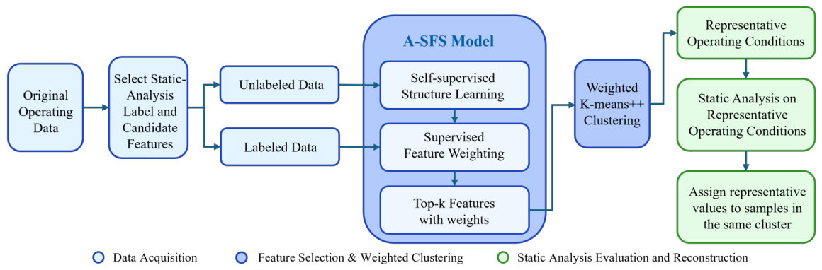
Figure 1 illustrates the overall workflow of the proposed framework. After the original operating data are collected, the preprocessing step first specifies the downstream static-analysis label and constructs the corresponding candidate feature set manually based on the physical relevance of operating-condition variables to the specified label. Target values are then calculated only for a partial subset to form labeled data, while the remaining operating conditions are retained as unlabeled data for semi-supervised feature selection. Next, A-SFS is employed to learn label-relevant feature representations and generate feature-importance weights. Based on the selected features and learned weights, all operating conditions, including both labeled and unlabeled samples, are mapped into a reduced label-relevant feature space, where weighted K-means++ is performed with a prescribed representative-scenario number. In this way, the reduction stage is guided by the designated static-analysis target without requiring target-value calculation for every operating condition in the annual dataset. Subsequently, static power-system analysis is carried out only for the selected representative scenarios, and the obtained target values are assigned to the operating conditions within the same clusters to reconstruct the overall target-value profile of the full dataset.

2.1. Data Representation and Problem Formulation

The annual operating-condition dataset is represented as

$$\mathbf{X}=\left[\begin{array}{c}{\mathbf{x}}_1^{\top }\\ {\mathbf{x}}_2^{\top }\\ ⋮\\ {\mathbf{x}}_N^{\top }\end{array}\right]\in {\mathbb{R}}^{N\times d},$$

(1)

where each row corresponds to one hourly operating condition and each column corresponds to one system feature. Depending on the specific study setting, the feature vector may include active and reactive load levels, generator outputs, renewable injections, bus voltages, line-flow quantities, or other steady-state descriptors relevant to static power-system analysis.

To eliminate scale inconsistency among heterogeneous physical variables, each feature is normalized before feature selection and clustering. In this framework, min–max normalization is adopted:

$${\tilde{x}}_{tj}={\displaystyle \frac{x_{tj}-x_j^{min}}{x_j^{max}-x_j^{min}+ϵ}},$$

(2)

where $x_{tj}$ is the value of the j-th feature of the t-th operating condition, $x_j^{min}$ and $x_j^{max}$ are the minimum and maximum values of the j-th feature over the dataset, and $ϵ$ is a small positive constant to avoid division by zero. The normalized dataset is denoted by $\tilde{\mathbf{X}}$.

Since computing static-analysis target values for all operating conditions can be time-consuming, only a partial subset of operating conditions is labeled. Let ${\mathcal{I}}_l$ and ${\mathcal{I}}_u$ denote the index sets of labeled and unlabeled samples, respectively:

$${\mathcal{I}}_l\cup {\mathcal{I}}_u=\{1,2,\dots ,N\},{\mathcal{I}}_l\cap {\mathcal{I}}_u=⌀,$$

(3)

where $|{\mathcal{I}}_l|=N_l$, $|{\mathcal{I}}_u|=N_u$, and $N_l+N_u=N$. The labeled ratio is defined as

$$\rho ={\displaystyle \frac{N_l}{N}}.$$

(4)

In the proposed framework, $\rho$ is treated as a prescribed labeled-data ratio, which provides target information for supervised feature-relevance learning while avoiding target-value calculation for the entire annual dataset during the feature-selection stage.

The labeled subset is defined as

$${\mathcal{D}}_l=\{({\tilde{\mathbf{x}}}_i,y_i)\mid i\in {\mathcal{I}}_l\},$$

(5)

where $y_i$ is the static-analysis target value computed for the i-th operating condition. The unlabeled subset is defined as

$${\mathcal{D}}_u=\{{\tilde{\mathbf{x}}}_i\mid i\in {\mathcal{I}}_u\}.$$

(6)

The unlabeled subset does not require target-value calculation and is used for self-supervised structure learning.

The goal of the proposed problem-driven scenario reduction is to identify a reduced scenario set

$$\mathcal{R}=\{{\mathbf{r}}_1,{\mathbf{r}}_2,\dots ,{\mathbf{r}}_M\},M\ll N,$$

(7)

such that static-analysis calculations are only required for this reduced set, while the obtained representative target values can be used to approximate the target values of the remaining operating conditions in the same clusters. Here, M denotes the prescribed number of representative scenarios. The key difference from conventional scenario reduction is that the clustering space is not defined only by geometric similarity in the original feature space, but is guided by the static-analysis target through learned feature weights.

2.2. A-SFS-Based Label-Relevant Feature Selection

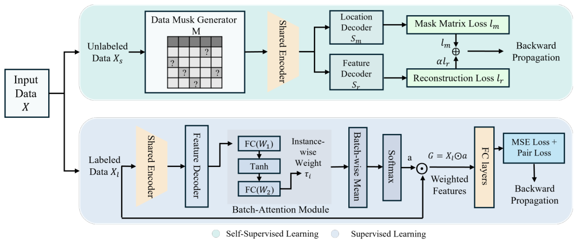
The overall structure of the A-SFS-based target-aware weighting model is shown in Figure 2. A-SFS was originally proposed as a semi-supervised feature-selection model that combines self-supervised representation learning with supervised feature-importance estimation [22]. As illustrated in Figure 2, the upper branch employs unlabeled operating-condition data to learn latent feature representations through a shared encoder and dual reconstruction objectives, while the lower branch utilizes partially labeled data to estimate target-relevant feature weights through the batch-attention module. The learned feature weights are subsequently used to construct a weighted feature space for representative operating-condition selection. To effectively capture the relative target-space structure inherent in operating conditions, we further incorporate a pairwise target-distance-preserving loss into the supervised learning stage.

2.2.1. Self-Supervised Structure Learning

A-SFS is used to discover label-relevant features from operating-condition data in a semi-supervised manner. Its core idea is to first learn latent structural relationships among features from the unlabeled operating conditions, and then use the labeled data to convert such structural knowledge into feature-importance weights.

Let $\mathbf{x}\in {\mathbb{R}}^d$ be one normalized operating condition. A masking operator is first applied to generate a corrupted input:

$${\mathbf{x}}^{\mathrm{mask}}=R(\mathbf{x},\mathbf{m})=\mathbf{m}\odot \overline{\mathbf{x}}+(1-\mathbf{m})\odot \mathbf{x},$$

(8)

where $\mathbf{m}\in {\{0,1\}}^d$ is a random binary mask vector, $\overline{\mathbf{x}}$ is the replacement vector sampled from the same feature distribution, and ⊙ denotes element-wise multiplication. This masking mechanism encourages the network to recover both feature values and feature positions from incomplete inputs.

A shared encoder $E(·)$ and two decoders are then constructed. The first decoder predicts the mask locations, while the second decoder reconstructs the masked feature values. Denote by $\widehat{\mathbf{m}}$ the estimated mask vector and by $\widehat{\mathbf{x}}$ the reconstructed feature vector:

$$\widehat{\mathbf{m}}=S_m\left(E\left({\mathbf{x}}^{\mathrm{mask}}\right)\right),\widehat{\mathbf{x}}=S_r\left(E\left({\mathbf{x}}^{\mathrm{mask}}\right)\right),$$

(9)

where $S_m(·)$ and $S_r(·)$ represent the mask-estimation decoder and feature-reconstruction decoder, respectively.

The self-supervised pretraining objective is formulated as

$${\mathcal{L}}_{\mathrm{ss}}={\mathcal{L}}_m(\mathbf{m},\widehat{\mathbf{m}})+\alpha {\mathcal{L}}_r(\mathbf{x},\widehat{\mathbf{x}}),$$

(10)

where $\alpha$ is a balancing coefficient. The mask-estimation loss is defined as binary cross-entropy:

$${\mathcal{L}}_m=-{\displaystyle \frac{1}{d}}{\displaystyle \sum _{j=1}^d}\left[m_{j}log{\widehat{m}}_j+(1-m_j)log(1-{\widehat{m}}_j)\right],$$

(11)

and the reconstruction loss is defined as mean squared error:

$${\mathcal{L}}_r={\displaystyle \frac{1}{d}}{\displaystyle \sum _{j=1}^d}{(x_j-{\widehat{x}}_j)}^2.$$

(12)

Through minimizing (10) over the unlabeled subset, the encoder learns feature interactions and latent structural patterns embedded in the annual operating-condition dataset without requiring target values for all samples.

2.2.2. Batch-Attention Feature Weight Generation

After self-supervised pretraining, the learned encoder is transferred to the supervised feature-selection stage. For each labeled sample ${\mathbf{x}}_i$ in ${\mathcal{D}}_l$, an attention transformation network is applied to generate an instance-wise score vector:

$${\tau }_i={\mathbf{W}}_{2}tanh\left({\mathbf{W}}_1(S_r\circ E)\left({\mathbf{x}}_i\right)+{\mathbf{b}}_1\right)+{\mathbf{b}}_2,$$

(13)

where ${\mathbf{W}}_1$, ${\mathbf{W}}_2$, ${\mathbf{b}}_1$, and ${\mathbf{b}}_2$ are trainable parameters.

To improve robustness against noisy samples, A-SFS uses batch-wise rather than instance-wise feature weighting. For a labeled mini-batch of size B, the score vectors are averaged as

$$\overline{\tau }={\displaystyle \frac{1}{B}}{\displaystyle \sum _{i=1}^B}{\tau }_i.$$

(14)

The feature-importance vector is then obtained using the softmax operator:

$$\mathbf{a}=\mathrm{softmax}\left(\overline{\tau }\right),a_j={\displaystyle \frac{exp\left({\overline{\tau }}_j\right)}{{\sum }_{q=1}^{d}exp\left({\overline{\tau }}_q\right)}},$$

(15)

where $a_j$ denotes the importance weight of the j-th feature. A larger $a_j$ indicates stronger relevance of feature j to the designated label value.

The learned weight vector is applied to the labeled samples through element-wise weighting:

$${\mathbf{g}}_i=\mathbf{a}\odot {\mathbf{x}}_i.$$

(16)

2.2.3. Supervised Regression and Pairwise Target-Distance Preserving Loss

A regression evaluation network $f(·)$ is first used to connect feature selection with the downstream static-analysis label. For the i-th labeled sample in a mini-batch, the predicted label is written as

$${\widehat{y}}_i=f\left({\mathbf{g}}_i\right),$$

(17)

where ${\mathbf{g}}_i$ is the attention-weighted feature vector. Since the static-analysis targets considered in this paper are continuous variables, the regression loss is defined on the labeled mini-batch as

$${\mathcal{L}}_{\mathrm{reg}}={\displaystyle \frac{1}{B}}{\displaystyle \sum _{i=1}^B}{\left({\widehat{y}}_i-y_i\right)}^2.$$

(18)

Although the regression loss encourages the selected features to carry target-relevant information, it mainly constrains each labeled operating condition independently. However, scenario reduction is essentially a distance-based grouping problem, where the relative relationship among operating conditions also affects the final representative scenarios. Therefore, a pairwise target-distance preserving loss is further introduced to make the learned weighted feature space more consistent with the target-value space.

For a pair of labeled samples $({\mathbf{x}}_i,y_i)$ and $({\mathbf{x}}_j,y_j)$ in the same labeled mini-batch, the weighted feature-space distance is defined as

$$D_{ij}^x=\sqrt{\sum _{p=1}^d{a}_p{\left(x_{ip}-x_{jp}\right)}^2+ϵ},$$

(19)

where $a_p$ is the learned importance weight of the p-th feature, and $ϵ$ is a small positive constant for numerical stability. The corresponding target-space distance is defined as

$$D_{ij}^y=\left|y_i-y_j\right|.$$

(20)

To avoid scale mismatch between feature-space distances and target-space distances, both distances are normalized within each labeled mini-batch. Let

$${\overline{D}}^x={\displaystyle \frac{2}{B(B-1)}}\sum _{1\le i<j\le B}{D}_{ij}^x,{\overline{D}}^y={\displaystyle \frac{2}{B(B-1)}}\sum _{1\le i<j\le B}{D}_{ij}^y.$$

(21)

The pairwise target-distance preserving loss is then formulated as

$${\mathcal{L}}_{\mathrm{pair}}={\displaystyle \frac{2}{B(B-1)}}\sum _{1\le i<j\le B}{\left({\displaystyle \frac{D_{ij}^x}{{\overline{D}}^x+ϵ}}-{\displaystyle \frac{D_{ij}^y}{{\overline{D}}^y+ϵ}}\right)}^2.$$

(22)

The supervised learning objective is finally defined as

$${\mathcal{L}}_{\sup }={\mathcal{L}}_{\mathrm{reg}}+{\lambda }_{\mathrm{pair}}{\mathcal{L}}_{\mathrm{pair}},$$

(23)

where ${\lambda }_{\mathrm{pair}}$ is a non-negative hyperparameter controlling the contribution of pairwise target-distance preservation. The regression loss is assigned a unit coefficient and serves as the primary supervised objective. When ${\lambda }_{\mathrm{pair}}=0$, the supervised objective degenerates to the original regression-based A-SFS training objective.

By incorporating both the regression loss and the pairwise target-distance preserving loss, the learned feature weights are encouraged not only to capture target-relevant value variations, but also to preserve the relative target-space relationships among labeled operating conditions. This is consistent with the subsequent weighted clustering stage, because operating conditions with similar static-analysis labels are expected to be closer in the learned weighted feature space.

After supervised training, A-SFS produces a ranked list of features together with their relative importance. Denote the selected feature subset by

$$\mathcal{S}={\mathrm{Top}}_k\left(\mathbf{a}\right),$$

(24)

where $\mathcal{S}$ contains the k most important features according to $\mathbf{a}$. Here, k denotes the prescribed number of selected features and is treated as a feature-selection hyperparameter. The corresponding reduced feature matrix for all operating conditions is

$$\mathbf{Z}=\tilde{\mathbf{X}}(:,\mathcal{S})\in {\mathbb{R}}^{N\times k}.$$

(25)

This reduced matrix contains both labeled and unlabeled samples and serves as the input to the subsequent weighted clustering stage.

2.3. Weighted K-Means++ for Scenario Reduction

After label-relevant feature selection, scenario reduction is carried out for all operating conditions in the reduced feature space $\mathbf{Z}$. Let ${\mathbf{z}}_i\in {\mathbb{R}}^k$ denote the reduced feature vector of the i-th operating condition, and let $\mathbf{w}={[w_1,\dots ,w_k]}^{\top }$ be the normalized weight vector associated with the selected features, obtained from the corresponding entries of $\mathbf{a}$. The number of clusters in weighted K-means++ is set to the prescribed representative-scenario number M.

To reflect unequal feature importance in clustering, the conventional Euclidean distance is replaced by a weighted Euclidean distance:

$$d_w({\mathbf{z}}_i,{\mathsf{\mu }}_c)=\sqrt{\sum _{j=1}^k{w}_j{\left(z_{ij}-{\mu }_{cj}\right)}^2},$$

(26)

where ${\mathsf{\mu }}_c$ is the centroid of cluster $C_c$. In this way, variations along features that are more relevant to the label value have a larger influence on the clustering process.

To improve initialization quality, K-means++ seeding is adopted. The first centroid is selected randomly from the dataset. Each subsequent centroid is sampled with probability proportional to the squared weighted distance from the nearest already selected centroid:

$$P\left({\mathbf{z}}_i\right)={\displaystyle \frac{D_w{\left({\mathbf{z}}_i\right)}^2}{{\sum }_{n=1}^N{D}_w{\left({\mathbf{z}}_n\right)}^2}},$$

(27)

where $D_w\left({\mathbf{z}}_i\right)$ denotes the weighted distance from ${\mathbf{z}}_i$ to its nearest selected centroid.

Given the initialized centroids, weighted K-means++ iteratively updates cluster assignments and centroids by minimizing the weighted within-cluster sum of squares:

$$J={\displaystyle \sum _{c=1}^M}\sum _{{\mathbf{z}}_i\in C_c}{\displaystyle \sum _{j=1}^k}{w}_j{\left(z_{ij}-{\mu }_{cj}\right)}^2.$$

(28)

For fixed assignments, the j-th component of the c-th centroid is updated by

$${\mu }_{cj}={\displaystyle \frac{1}{|C_c|}}\sum _{{\mathbf{z}}_i\in C_c}{z}_{ij}.$$

(29)

The assignment and update steps are repeated until convergence.

After convergence, the original annual operating-condition set is partitioned into M clusters:

$$\mathcal{C}=\{C_1,C_2,\dots ,C_M\}.$$

(30)

It should be noted that the centroid ${\mathsf{\mu }}_c$ obtained by K-means++ is generally a virtual point in the reduced feature space rather than an actual operating condition. Therefore, to ensure that each representative scenario corresponds to a physically realizable operating condition, the actual sample closest to the centroid is selected as the representative scenario of each cluster:

$$i_c^{*}=arg\underset{i:{\mathbf{z}}_i\in C_c}{min}{d}_w({\mathbf{z}}_i,{\mathsf{\mu }}_c),$$

(31)

and the corresponding representative operating condition is

$${\mathbf{r}}_c={\mathbf{x}}_{i_c^{*}},$$

(32)

where ${\mathbf{x}}_{i_c^{*}}$ denotes the original operating condition associated with the selected reduced-space sample ${\mathbf{z}}_{i_c^{*}}$.

The final reduced scenario set is then written as

$$\mathcal{R}=\{{\mathbf{r}}_1,{\mathbf{r}}_2,\dots ,{\mathbf{r}}_M\}.$$

(33)

For subsequent static-analysis evaluation, the target value of each representative operating condition can be calculated if it is not already available. The representative target value is then assigned to the operating conditions in the same cluster, thereby reconstructing the overall static-analysis target profile of the full operating-condition dataset.

Compared with conventional clustering directly applied to the original feature space, the proposed weighted K-means++ stage operates in a label-relevant reduced space learned by A-SFS. Moreover, by selecting the nearest actual operating condition rather than directly using the virtual centroid, the reduced scenario set remains physically meaningful and can be directly used in subsequent static power-system analysis.

3. Case Study

This section evaluates the proposed A-SFS-based problem-driven scenario reduction framework on a yearly static operating-condition dataset. The study is organized into four parts, namely data preparation, evaluation criteria, benchmark methods, and implementation details. Two representative static-analysis targets are considered in the experiments, i.e., load margin and the minimum singular value of the power-flow Jacobian. The corresponding results are reported separately to examine whether the proposed framework can use a limited number of representative operating conditions to reconstruct the overall annual target-value profile under different static security indicators.

3.1. Data Preparation

The case study is conducted on the Reliability Test System–Grid Modernization Laboratory Consortium (RTS-GMLC), which is a publicly available benchmark system designed to support modern power-system operation and planning studies [23]. The system includes a representative generation mix with conventional units, natural gas units, wind generation, solar photovoltaic generation, concentrating solar power, and energy storage. It also provides geographically consistent load, wind, and solar time-series data, which makes it suitable for constructing renewable-rich and time-varying operating conditions. During preprocessing, hourly load and generation profiles are mapped to the RTS-GMLC network model, and standard power-flow calculations are performed to construct feasible steady-state operating snapshots. The resulting operating-state variables, including bus voltage magnitudes, line-flow quantities, and inter-area transfers, are stored as part of the input feature matrix for scenario reduction. After preprocessing, a yearly set of static operating conditions is constructed, and each hourly operating point is treated as one sample. The final dataset contains 8760 hourly operating conditions. The corresponding operating-state variables are stored as the input feature matrix, while the static-analysis target values are treated separately.

Two representative static-analysis targets are considered in this study, including: load margin and the minimum singular value of the power-flow Jacobian, ${\sigma }_{min}$. These two targets are selected because they characterize different aspects of static voltage-stability-related operating conditions. Load margin reflects the distance between the current operating point and the corresponding critical loading condition, while ${\sigma }_{min}$ provides a compact Jacobian-based indicator of the local strength of the operating point. A smaller ${\sigma }_{min}$ generally indicates that the system is closer to Jacobian singularity and therefore closer to voltage instability. Although only a partial labeled subset is used for feature-relevance learning and scenario reduction, the target values of all operating conditions are computed offline only for performance evaluation. In practical deployment, the full target set is not required by the proposed reduction process.

For the load margin task, the target value is calculated through power-flow-based loadability analysis, which evaluates the distance from the current operating point to the corresponding critical loading condition. The candidate feature set is composed of bus active and reactive power demands, generator active and reactive power outputs, active and reactive power flows on key transmission lines, and inter-area active and reactive power transfers. These variables are selected because load margin is closely related to system loading level, generation redispatch pattern, and power-transfer condition.

For the minimum singular value of the power-flow Jacobian task, the target value is calculated from the power-flow Jacobian matrix at each solved operating point. Specifically, after the power-flow solution is obtained for a labeled operating condition, the corresponding Jacobian matrix is formed, and its minimum singular value is computed as ${\sigma }_{min}$. The candidate feature set is composed of bus active and reactive power demands, generator active and reactive power outputs, generator reactive power reserves, bus voltage magnitudes, active and reactive power flows on key transmission lines, and inter-area active and reactive power transfers. Compared with the load-margin task, voltage magnitudes and reactive power reserves are additionally included because ${\sigma }_{min}$ is more directly related to local voltage-stability strength and reactive-power support.

3.2. Evaluation Criteria

Since the goal of the proposed framework is not merely to compress the operating-condition set, but to preserve target-relevant information for downstream static analysis, two complementary evaluation metrics are adopted.

The first metric is the global mean absolute percentage error (MAPE). After clustering, every original operating condition is represented by the label value of its assigned representative scenario. Let $c\left(t\right)$ denote the representative scenario associated with sample t, and let ${\widehat{y}}_t$ be the reconstructed target value:

$${\widehat{y}}_t=y_{c\left(t\right)}.$$

(34)

Then the global MAPE is computed as

$$\mathrm{MAPE}={\displaystyle \frac{1}{N}}{\displaystyle \sum _{t=1}^N}\left|{\displaystyle \frac{y_t-{\widehat{y}}_t}{y_t}}\right|\times 100\%.$$

(35)

This metric evaluates the numerical discrepancy between the reconstructed and actual target-value profiles over all 8760 operating conditions from a global reconstruction perspective.

The second metric is the Spearman rank correlation coefficient, which evaluates whether the reduction process preserves the global ordering of operating conditions with respect to the target value:

$${\rho }_s=\mathrm{corr}\left(\mathrm{rank}\left(\mathbf{y}\right),\mathrm{rank}\left(\widehat{\mathbf{y}}\right)\right),$$

(36)

where $\mathbf{y}={[y_1,\dots ,y_N]}^{\top }$ and $\widehat{\mathbf{y}}={[{\widehat{y}}_1,\dots ,{\widehat{y}}_N]}^{\top }$. This metric is particularly important for the present study because the proposed method is designed in a target-oriented manner. For planning-oriented static-analysis studies, preserving the relative ranking is important because it helps retain the ordering of operating conditions with respect to the target value, so that potentially weak or stressed operating regions can still be revealed after scenario reduction.

Taken together, MAPE measures the fidelity of numerical reconstruction, while Spearman correlation measures the preservation of global ordering. The two metrics therefore provide a more complete assessment of whether the reduced scenario set remains useful for downstream static power-system analysis.

3.3. Benchmark Methods

To demonstrate the effectiveness of the proposed framework, four benchmark methods are considered.

• Benchmark A: K-means++. This benchmark directly performs K-means++ clustering in the normalized original feature space. It serves as the most basic clustering-based scenario reduction baseline without dimension reduction.
• Benchmark B: PCA + K-means++. This benchmark first applies principal component analysis (PCA) for unsupervised dimensionality reduction and then performs K-means++ in the transformed feature space [13]. It represents a conventional pipeline in which dimensionality reduction is conducted independently of the downstream static-analysis target.
• Benchmark C: RRelief + PSO-K-means. This benchmark follows the target-related feature-weighting and clustering strategy adopted in [17]. First, RRelief is used to evaluate feature relevance. Then particle swarm optimization (PSO) is employed together with K-means to search for a more suitable clustering structure. This benchmark is one of the most relevant target-aware reduction methods in the literature and is closely related to planning-oriented fast stability scanning.
• Benchmark D: Scenario Reduction Network (SRN). This benchmark adopts the neural scenario reduction model proposed in [14], which formulates scenario reduction through a regularized Wasserstein-distance objective and learns representative scenarios in an unsupervised manner. Compared with conventional clustering baselines, SRN provides a stronger data-driven scenario reduction benchmark.

The main parameter settings of the benchmark methods are summarized in

Table 1. Main algorithmic parameter settings of the benchmark scenario-reduction methods.

Benchmark Method	Parameter/Setting	Selected Value
PCA + K-means++	Cumulative explained variance retained by PCA	$95\%$
SRN	Regularization coefficient $ϵ$	${10}^{-2}$
	Learning rate	$0.02$
	Maximum/minimum training epochs	1000/100
RReliefF + self-adaptive PSO-K-means	Number of nearest neighbors in RReliefF	20
	RReliefF distance-decay parameter $\sigma$	$10.0$
	Number of retained features	120
	Weight-adjustment coefficient C	$1.0$
	Initial cluster number $K_0$	400
	Swarm size	20
	Maximum PSO iterations	60
	Inertia-weight range	$0.9$–$0.4$
	Acceleration coefficients	$c_1=c_2=2.0$
	Maximum adaptive-mutation probability	$0.2$
	Data-distance threshold ${\Delta }_d$	$0.95$
	Centroid-merge threshold ${\Delta }_c$	$0.01$

.

3.4. Implementation Details

All experiments are implemented in Python 3.11.9, and the learning-based modules are built with PyTorch 2.7.1. The experiments are conducted on a workstation equipped with an Intel(R) Core(TM) i9-13900HX CPU and an NVIDIA GeForce RTX 4060 GPU. To ensure a fair comparison, the same yearly dataset, preprocessing procedure, feature categories, and evaluation protocol are used for all methods.

For the A-SFS learning stage, 20% of the annual operating-condition samples are randomly selected as labeled data, while the remaining 80% are used as unlabeled data. This setting is motivated by the labeled-data proportion adopted in the original A-SFS study, where the labeled-data portions in the public-dataset experiments are approximately within the range of 11.5–25.0% [22]. The labeled subset is further divided into a supervised training set and a validation set with a ratio of 80%:20%. The validation set is used for early stopping and model selection. After the feature weights are obtained, scenario reduction is performed on the full annual operating-condition dataset. The final MAPE and Spearman coefficients are evaluated over the full annual dataset using the offline-computed target values.

The main parameter settings of the proposed A-SFS-based feature-selection module are summarized in

Table 2. Main parameter settings and selection basis of the proposed A-SFS-based feature-selection module.

Parameter/Setting	Selected Value	Selection Basis
Unlabeled batch size	128	Adopted from the original A-SFS configuration.
Masking probability	$0.2$	Adopted from the original A-SFS configuration.
Encoder hidden dimension	128	Selected to provide sufficient representation capacity while avoiding an oversized encoder for the present dataset.
Reconstruction-loss weight $\alpha$	$2.0$	Adopted from the original A-SFS configuration.
Pretraining learning rate	$5\times {10}^{-4}$	Reduced from the original setting to improve convergence stability on numerical power-system operating data.
Number of pretraining epochs	100	Determined according to the convergence behavior of the self-supervised pretraining loss.
Labeled batch size	128	Adopted from the original A-SFS configuration.
Attention hidden dimension	300	Adopted from the original A-SFS configuration.
Regression-network hidden dimension	128	Selected as a compact regression head to balance nonlinear fitting ability and overfitting risk.
Supervised learning rate	$5\times {10}^{-5}$	Chosen to ensure stable supervised training after the self-supervised pretraining stage.
Number of supervised-training epochs	1000	Determined according to the convergence of the supervised loss and validation performance.
Regression-loss weight ${\lambda }_{\mathrm{reg}}$	$1.0$	Used as the reference supervised regression objective in the combined loss function.
Pairwise-loss weight ${\lambda }_{\mathrm{pair}}$	$0.003$ for load margin; $0.005$ for ${\sigma }_{min}$	Selected according to the target-specific sensitivity analysis, as analyzed in Section 3.5.
Number of selected features k	30	Chosen to obtain a compact feature subset while retaining sufficient target-relevant information for scenario reduction.

. Parameters whose selection basis refers to the original A-SFS configuration follow or are adapted from the original A-SFS implementation [22], while the remaining task-specific parameters were determined according to convergence behavior, validation performance, or sensitivity analysis.

Two comparison protocols are adopted in the case study. First, a fixed-M comparison is conducted at $M=300$, 400, and 500 for the methods whose representative-scenario number can be directly prescribed, including Benchmark A, Benchmark B, Benchmark D, and the proposed method. Benchmark C is not included in the fixed-M comparison because it adaptively determines the number of clusters during its optimization process. Therefore, the fixed-M comparison is used to evaluate the target-value profile reconstruction of controllable-M methods under the same reduced-set size, which corresponds to the same static-analysis computational budget.

Second, a best-M comparison is conducted for all methods, including Benchmark C. For each method, the result with the lowest MAPE is selected from the tested representative-scenario numbers within the range of 300–500, and the corresponding Spearman coefficient is reported under the same M. This comparison is used to evaluate the best target-value profile reconstruction performance that each method can achieve within the tested reduced-set sizes. It should be noted that the proposed method does not automatically determine the optimal number of representative scenarios; M is treated as a prescribed experimental setting throughout this study.

3.5. Sensitivity Analysis of ${\lambda }_{\mathrm{pair}}$

The pairwise-loss weight ${\lambda }_{\mathrm{pair}}$ controls the contribution of the target-distance preserving term in the supervised training stage. Since this term directly affects the feature weights learned by the A-SFS module and the subsequent weighted K-means++ clustering results, a sensitivity analysis was conducted to determine an appropriate value of ${\lambda }_{\mathrm{pair}}$ for each static-analysis target.

In this analysis, ${\lambda }_{\mathrm{pair}}$ was varied within the candidate set

$${\lambda }_{\mathrm{pair}}\in \{0,0.0005,0.001,0.003,0.005,0.01,0.03,0.05,0.1\}.$$

(37)

Here, ${\lambda }_{\mathrm{pair}}=0$ represents the ablation case without the pairwise target-distance preserving loss, and is used to examine the contribution of this loss term. For each candidate value of ${\lambda }_{\mathrm{pair}}$, all other hyperparameters were kept unchanged, while the representative-scenario number M was tested at 300, 400, and 500. The complete scenario-reduction pipeline was repeated for each M, including A-SFS-based feature selection, weighted K-means++ clustering, and representative-scenario reconstruction. The final sensitivity result for each ${\lambda }_{\mathrm{pair}}$ was summarized by averaging the MAPE values and Spearman coefficients over the three tested M values.

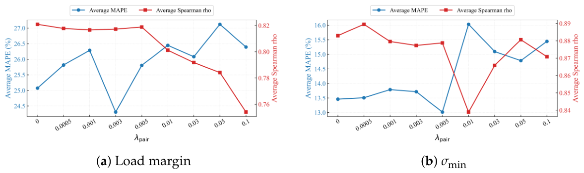
As shown in Figure 3, the performance of the proposed framework depends on the balance between the regression loss and the pairwise target-distance preserving loss. When ${\lambda }_{\mathrm{pair}}$ is too small, the target-distance preserving effect is insufficient. In contrast, an excessively large value of ${\lambda }_{\mathrm{pair}}$ overemphasizes the pairwise loss and may deteriorate the final reconstruction accuracy. Therefore, a moderate value of ${\lambda }_{\mathrm{pair}}$ is preferred.

For the load-margin task, ${\lambda }_{\mathrm{pair}}=0.003$ achieves the lowest average MAPE while maintaining a comparable Spearman correlation coefficient. Compared with the ablation case ${\lambda }_{\mathrm{pair}}=0$, the average MAPE is reduced from 25.07% to 24.30%. For the ${\sigma }_{min}$ task, ${\lambda }_{\mathrm{pair}}=0.005$ gives the lowest average MAPE while maintaining a high Spearman correlation coefficient, reducing the average MAPE from 13.46% to 13.01% compared with ${\lambda }_{\mathrm{pair}}=0$. Therefore, these task-specific values are adopted in the following experiments. These results indicate that the pairwise target-distance preserving loss improves the target-value profile reconstruction when its weight is properly selected.

3.6. Results for Load Margin

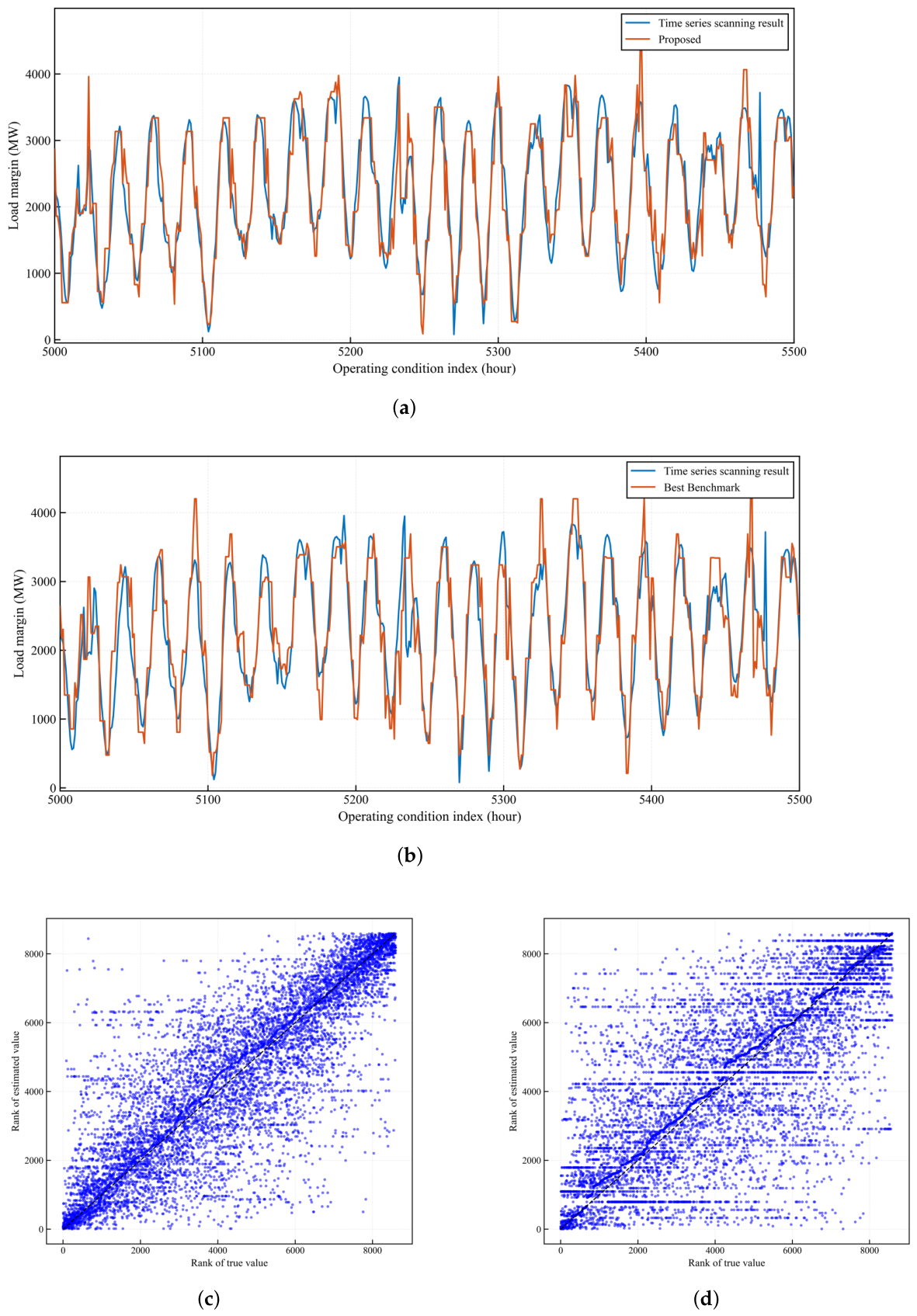
Figure 4 provides a visual comparison between the reconstructed load-margin profile and the time-series scanning result. As shown in Figure 4b, the benchmark model generally captures the overall periodic trend of the load margin. However, noticeable deviations can be observed in several high-fluctuation intervals and near local extrema. These deviations are mainly reflected in local amplitude mismatches and occasionally flattened or abrupt local fluctuations. This indicates that the benchmark model is less effective in representing rapidly varying or extreme operating conditions. By contrast, the proposed model in Figure 4a follows the scanning-based load-margin trajectory more closely over most operating conditions. The improvement is especially evident in the high-fluctuation intervals, where the proposed model better preserves the temporal variation pattern and the amplitude of the load-margin changes. Nevertheless, small local discrepancies can still be observed near abrupt transitions and extreme operating points. Therefore, the proposed model provides a more consistent reconstruction of the overall load-margin profile.

Figure 4c,d further compare the rank relationship between the true and reconstructed load-margin values. The scatter plot of the proposed method shows a clearer increasing trend and a more concentrated distribution around the diagonal direction, indicating better preservation of the relative ordering of operating conditions. By comparison, the benchmark result exhibits more dispersed rank points, suggesting weaker rank preservation after scenario reduction.

Table 3. Comparison results on Load Margin under different representative scenario numbers.

Metric	Method	$\mathit{M}=300$	$\mathit{M}=400$	$\mathit{M}=500$
MAPE ↓	Benchmark A	33.21%	30.56%	28.98%
	Benchmark B	32.95%	29.50%	28.35%
	Benchmark D	35.47%	32.73%	30.79%
	Proposed	29.42%	22.49%	21.10%
Spearman coefficient ↑	Benchmark A	0.6638	0.6636	0.6976
	Benchmark B	0.6728	0.6948	0.7118
	Benchmark D	0.6774	0.6989	0.7240
	Proposed	0.7882	0.8250	0.8384

Note: Bold values indicate the best performance; ↓ means lower is better, and ↑ means higher is better.

reports the fixed-M comparison for the load-margin task. Under all three representative-scenario numbers, the proposed framework achieves the lowest MAPE and the highest Spearman coefficient. Specifically, when $M=300$, 400, and 500, the proposed method obtains MAPEs of $29.42\%$, $22.49\%$, and $21.10\%$, respectively, corresponding to absolute MAPE reductions of 3.53, 7.01, and 7.25 percentage points. The best benchmark MAPEs under the same settings are $32.95\%$, $29.50\%$, and $28.35\%$, respectively. Meanwhile, the proposed method also improves the Spearman coefficient to $0.7882$, $0.8250$, and $0.8384$, showing better preservation of the load-margin ranking structure.

The best-M comparison in

Table 4. Best-MAPE clustering results for load margin over the tested representative-scenario numbers.

Method	Best M	MAPE ↓	Spearman Coefficient ↑
Benchmark A	500	28.98%	0.6976
Benchmark B	500	28.35%	0.7118
Benchmark C	479	21.24%	0.7544
Benchmark D	500	30.79%	0.7240
Proposed	460	19.56%	0.8380

Note: Bold values indicate the best performance; ↓ means lower is better, and ↑ means higher is better.

further demonstrates the advantage of the proposed method. The proposed method reaches its best MAPE at $M=460$, where the MAPE is reduced to $19.56\%$. Compared with the strongest benchmark result, Benchmark C with a MAPE of $21.24\%$ at $M=479$, the proposed method provides an additional improvement of $1.68$ percentage points while using a smaller representative-scenario number. This result indicates that the proposed target-aware reduction strategy can retain more target-value information of the original operating-condition set even with a more compact reduced scenario set. The corresponding Spearman coefficient is $0.8380$, which is also higher than those of all benchmark methods. These results show that the proposed framework can better preserve both the numerical load-margin information and the relative ordering of operating conditions.

The robustness of the proposed method is examined by repeating the load-margin experiment using three independent random seeds. The corresponding MAPE and Spearman correlation coefficient are reported in

Table 5. Performance and result reliability of the proposed method for the load-margin task.

Model	MAPE (%)	Spearman Coefficient
Proposed (Run 1)	$19.04$	$0.8411$
Proposed (Run 2)	$19.34$	$0.8404$
Proposed (Run 3)	$20.31$	$0.8326$
Proposed (Mean ± SD)	$19.56\pm 0.66$	$0.8380\pm 0.0047$

. The proposed method shows stable performance across different runs, with MAPE values ranging from 19.04% to 20.31% and Spearman coefficients ranging from 0.8326 to 0.8411. The small standard deviations of both metrics indicate that the proposed A-SFS-based scenario reduction framework is not overly sensitive to random seed settings. Therefore, the improvement observed in the load-margin task is robust rather than being caused by a single favorable random run.

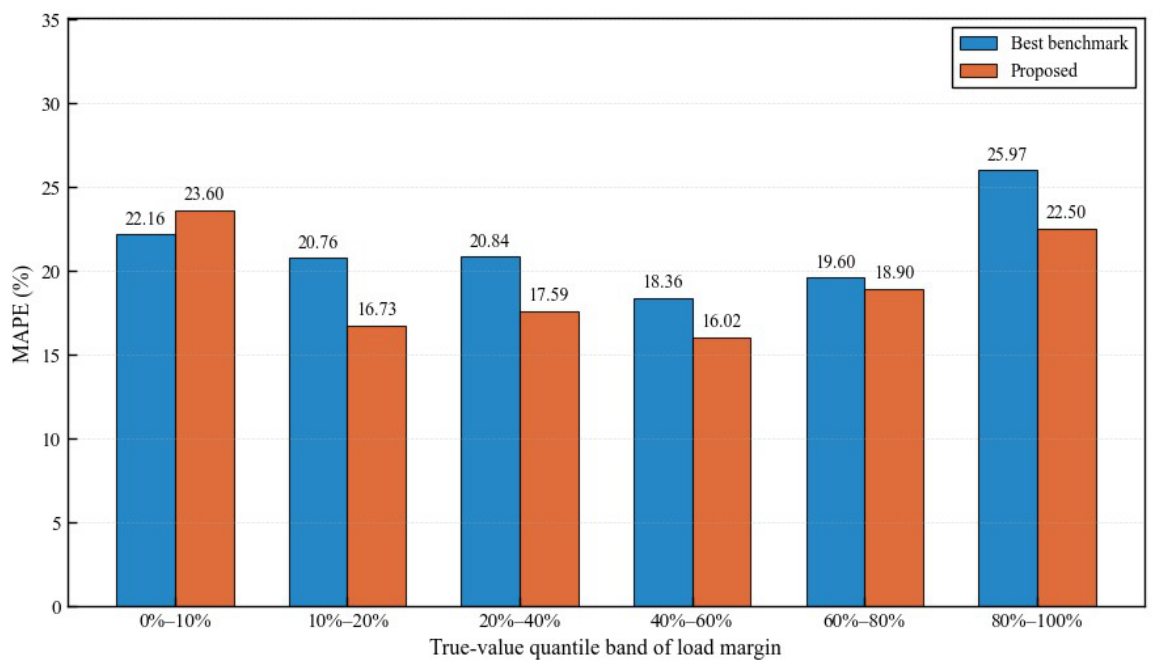
To further examine the reconstruction performance over different load-margin regions, the operating conditions are divided into six true-value quantile bands, and the MAPE is calculated separately for each band. As shown in Figure 5, the proposed method achieves lower MAPE than the best benchmark in most quantile bands, especially from the 10–20% band to the 80–100% band. This indicates that the proposed target-aware reduction strategy improves the reconstruction of the overall load-margin profile across a wide range of operating conditions. However, as shown in

Table 6. MAPE comparison in the low-value quantile bands for the load-margin task.

Method	0–10%	10–20%
Best benchmark	22.16%	20.76%
Proposed	23.60%	16.73%

, the proposed method shows a slightly higher MAPE in the lowest 0–10% band, suggesting that extremely low load-margin values remain more difficult to reconstruct accurately.

3.7. Results for the Minimum Singular Value of the Power-Flow Jacobian

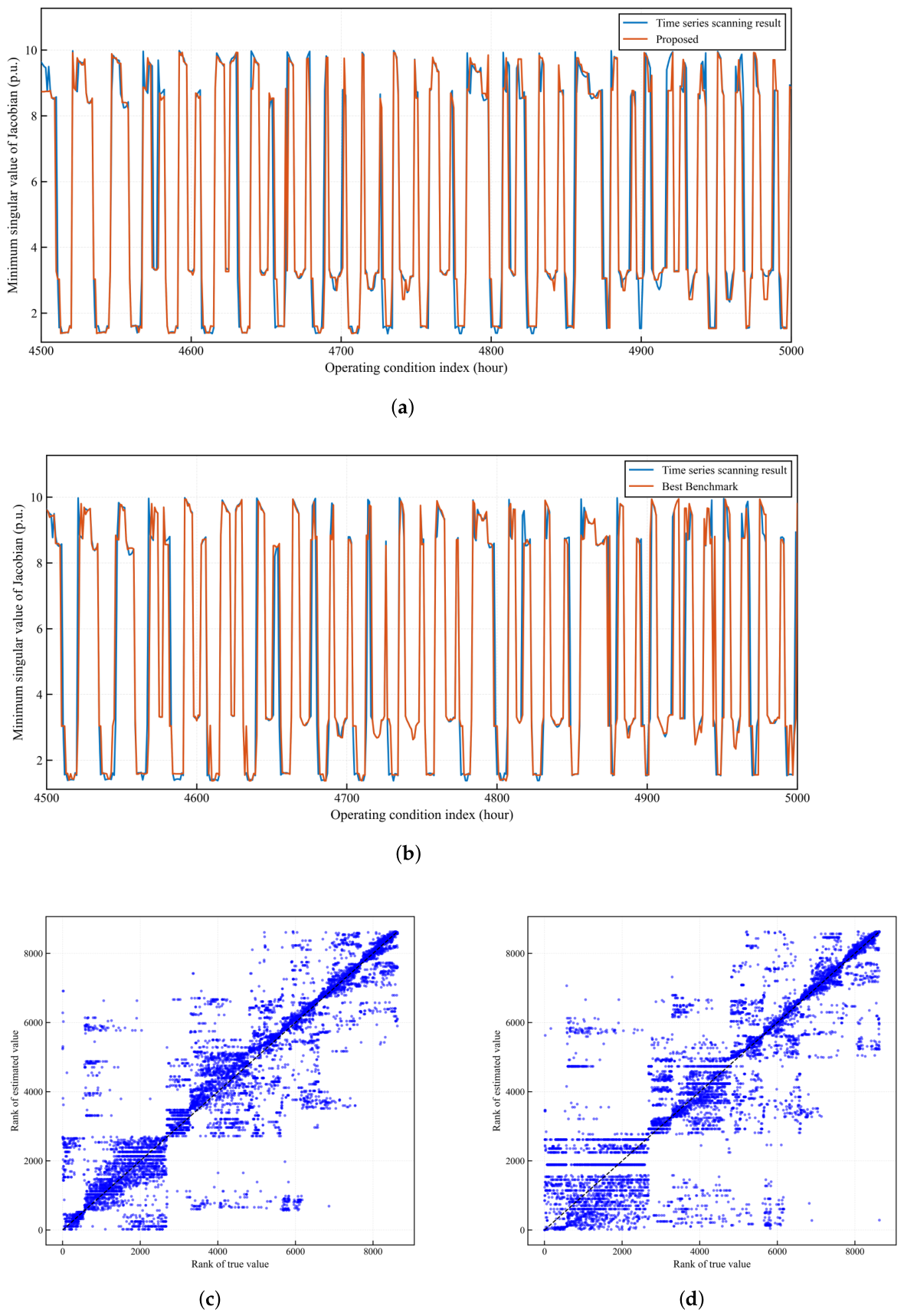
Figure 6 presents the visual comparison for the ${\sigma }_{min}$ task. As shown in Figure 6a,b, both methods can capture the overall periodic trend of the ${\sigma }_{min}$ profile, but the proposed method follows the time-series scanning result more closely in several high-fluctuation intervals and near local extrema. The benchmark method exhibits more visible amplitude mismatches and locally flattened fluctuations, indicating that it is less effective in representing rapidly varying operating conditions. The rank scatter plots in Figure 6c,d further show that the proposed method produces a clearer monotonic relationship between the true and reconstructed ranks, whereas the benchmark result is more dispersed. This suggests that the proposed target-aware reduction strategy better preserves both the main variation pattern and the relative ordering of ${\sigma }_{min}$ values.

Table 7. Comparison results on ${\sigma }_{min}$ under different representative scenario numbers.

Metric	Method	$\mathit{M}=300$	$\mathit{M}=400$	$\mathit{M}=500$
MAPE ↓	Benchmark A	15.51%	15.42%	15.18%
	Benchmark B	15.92%	14.46%	13.67%
	Benchmark D	16.35%	13.84%	15.72%
	Proposed	14.03%	12.83%	12.18%
Spearman coefficient ↑	Benchmark A	0.8484	0.8447	0.8618
	Benchmark B	0.8506	0.8628	0.8677
	Benchmark D	0.8512	0.8645	0.8601
	Proposed	0.8687	0.8789	0.8886

Note: Bold values indicate the best performance; ↓ means lower is better, and ↑ means higher is better.

reports the fixed-M comparison for the ${\sigma }_{min}$ task. The proposed framework achieves the best MAPE under all three representative-scenario numbers. Its MAPEs are $14.03\%$, $12.83\%$, and $12.18\%$ for $M=300$, 400, and 500, respectively, while the best benchmark MAPEs under the same settings are $15.51\%$, $13.84\%$, and $13.67\%$. The corresponding absolute improvements are $1.48$, $1.01$, and $1.49$ percentage points. In terms of Spearman coefficient, the proposed method also consistently obtains the highest values, reaching $0.8687$, $0.8789$, and $0.8886$. These results show that the proposed method is effective not only for load-margin reconstruction, but also for the Jacobian-based voltage-stability indicator.

The best-M comparison in

Table 8. Best-MAPE clustering results for ${\sigma }_{min}$ over the tested representative-scenario numbers.

Method	Best M	MAPE ↓	Spearman Coefficient ↑
Benchmark A	500	15.18%	0.8618
Benchmark B	500	13.67%	0.8677
Benchmark C	495	13.06%	0.8695
Benchmark D	400	13.84%	0.8645
Proposed	380	12.85%	0.8755

Note: Bold values indicate the best performance; ↓ means lower is better, and ↑ means higher is better.

leads to a similar conclusion. The proposed method achieves the lowest MAPE of $12.85\%$ at $M=380$, outperforming the best benchmark result of $13.06\%$ obtained by Benchmark C at $M=495$. This indicates that the proposed method can provide a more accurate reconstruction of the overall ${\sigma }_{min}$ profile while requiring fewer target evaluations. Since ${\sigma }_{min}$ reflects the local voltage-stability strength of operating conditions, better preservation of its overall profile and rank ordering can help planners compare the relative weakness of different operating regions more consistently during large-scale scanning. It also achieves the highest Spearman coefficient of $0.8755$, whereas the best benchmark value is $0.8695$. These results indicate that the proposed problem-driven reduction strategy can more effectively preserve both numerical reconstruction accuracy and rank-order information for ${\sigma }_{min}$, even under a more compact reduced scenario set.

The robustness of the proposed method was also evaluated for the ${\sigma }_{min}$ task using the same three random seeds. The corresponding MAPE and Spearman correlation coefficient are reported in

Table 9. Performance and result reliability of the proposed method for the ${\sigma }_{min}$ task.

Model	MAPE (%)	Spearman Coefficient
Proposed (Run 1)	12.14	0.8784
Proposed (Run 2)	13.32	0.8791
Proposed (Run 3)	13.09	0.8688
Proposed (Mean ± SD)	$12.85\pm 0.63$	$0.8755\pm 0.0058$

. The proposed method shows stable performance across different runs for the ${\sigma }_{min}$ task, with MAPE values ranging from 12.14% to 13.32% and Spearman coefficients ranging from 0.8688 to 0.8791. The small standard deviations of both metrics indicate that the proposed A-SFS-based scenario reduction framework is not overly sensitive to random seed settings for the ${\sigma }_{min}$ task.

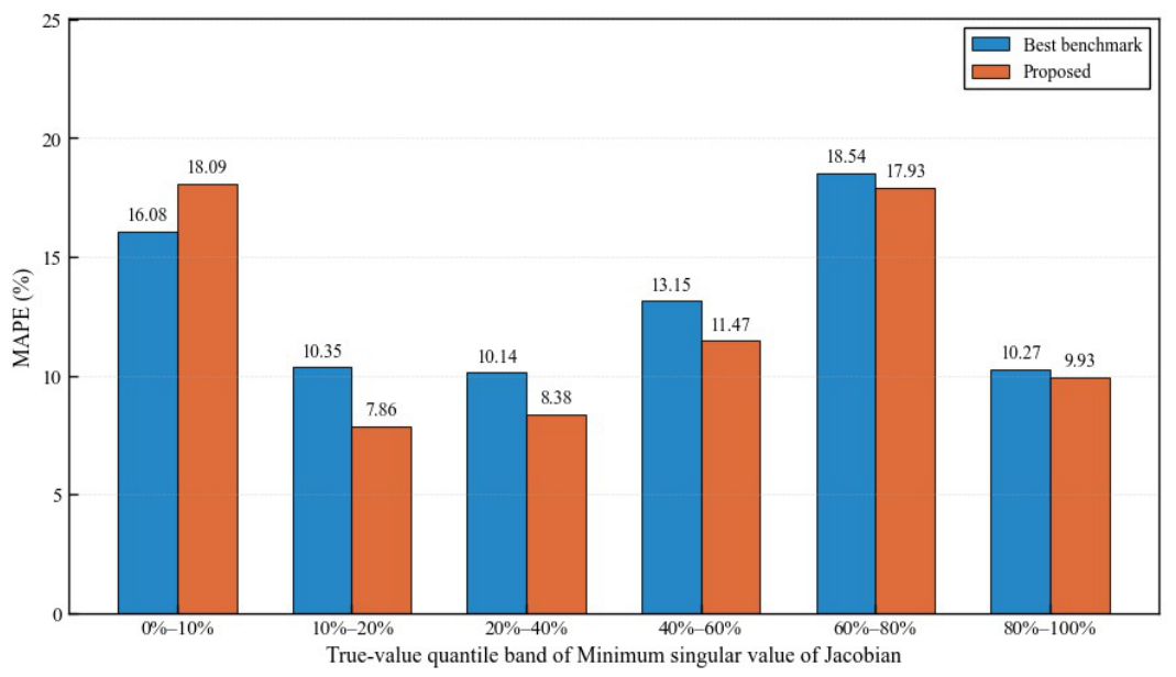
A similar quantile-band analysis is also conducted for the ${\sigma }_{min}$ task to evaluate whether the reconstruction error is concentrated in particular value regions. As shown in Figure 7, the proposed method obtains lower MAPE than the best benchmark in most quantile bands, especially in the 10–20%, 20–40%, and 40–60% bands. This indicates that the proposed target-aware reduction strategy can better reconstruct the overall ${\sigma }_{min}$ profile across a wide range of operating conditions. However, as shown in

Table 10. MAPE comparison in the low-value quantile bands for the ${\sigma }_{min}$ task.

Method	0–10%	10–20%
Best benchmark	16.08%	10.35%
Proposed	18.09%	7.86%

, the proposed method shows a slightly larger error in the lowest 0–10% band, suggesting that extremely small ${\sigma }_{min}$ values remain more difficult to reconstruct accurately.

4. Conclusions

This paper presented an A-SFS-based problem-driven scenario reduction framework for static power-system analysis. The main purpose of the proposed framework is to reduce the number of required downstream target-value evaluations while preserving the overall target-value profile of the original annual operating-condition dataset. Instead of selecting representative operating conditions only according to geometric similarity in the original feature space, the proposed method uses a partially labeled dataset to learn target-relevant feature weights and performs clustering in the resulting weighted feature space. In this way, the representative scenarios are selected according to their relevance to the designated static-analysis target, and their calculated target values are assigned to the corresponding clusters to reconstruct the overall target-value profile of the full operating-condition dataset. A pairwise target-distance preserving loss was further introduced to make the learned weighted feature space more consistent with the downstream clustering and reconstruction task.

The proposed framework was validated on the RTS-GMLC system using load margin and the minimum singular value of the power-flow Jacobian, ${\sigma }_{min}$, as two representative static-analysis targets. The results show that the proposed method can improve the reconstruction of the overall target-value profile and better preserve the relative ordering of operating conditions. The sensitivity analysis also confirms that an appropriate pairwise-loss weight can improve the balance between numerical profile reconstruction and rank preservation. These results indicate that the proposed framework is suitable for planning-level scanning of large annual operating-condition datasets. The robustness tests using three independent random seeds further show that the proposed method maintains stable MAPE and Spearman performance for both static-analysis targets, indicating that the observed improvements are not caused by a single favorable random run.

Several limitations remain. First, although the proposed method improves the global reconstruction performance and rank preservation, the quantile-band error analysis shows that extremely low load-margin values and extremely small ${\sigma }_{min}$ values are still more difficult to reconstruct accurately. This suggests that the current representative-scenario-based reconstruction strategy may provide insufficient fidelity for outlying low-value regions. Second, the present case study is conducted on the RTS-GMLC system and considers two static-analysis targets, so further validation on larger power-system models and additional security or stability indices is still needed. Future work will focus on improving the representation and reconstruction of extreme low-value operating regions, for example by exploring extreme-aware sampling and adaptive cluster-refinement strategies. In addition, the proposed framework will be tested on larger systems with more buses and more complex operating patterns to further evaluate its scalability and general applicability.