LAC-T: A Tutored Reinforcement Learning Framework of Hidden-Parameter Estimation for Health Monitoring of Rotating Systems

Abstract

Health status monitoring is critical for rotating systems to maintain safety and reliability. However, it is hard to track the health status hidden in unobservable parameters. Therefore, to address the issue of hidden-parameter estimation caused by the absence of critical sensors, this paper proposes an extended reinforcement learning framework named the Lyapunov Actor–Critic Tutor (LAC-T). In this framework, the LAC-T redefines parameter estimation in hidden health status monitoring as an observation–trajectory alignment problem rather than an observation–tracking problem, thereby maintaining the stability of the hidden-parameter estimation. Meanwhile, to address the multi-resolution problem in parameter estimation, a tutor component is introduced into the framework to guide parameter estimation. To validate the effectiveness and superiority of the proposed LAC-T framework, a case study including a motor torque coefficient estimation for a rotating system in a control moment gyroscope is investigated in this paper. The lower estimation error of the proposed LAC-T framework compared with the candidate problem definition and models indicates that the observation–trajectory alignment problem definition can stabilise the hidden-parameter estimation, and the tutor component can improve estimation accuracy, thereby improving the performance of hidden health status monitoring.

1. Introduction

As representative complex systems, rotating systems play a critical role in Industry 5.0 [1,2,3,4] and serve as the bridge among multiple physical fields to drive industrial processes [5,6]. Given the importance of rotating systems, assessing their health status both supports downstream operational decision-making and helps ensure the safety and reliability of industrial scenarios. For example, in applications such as dynamic maintenance scheduling, asset dispatching and industrial process optimisation, health status monitoring within the OODA framework [7] enables production lines to determine when maintenance should be performed, which assets should be dispatched to industrial sites, and how operating modes should be optimised to sustain longer and more efficient equipment operation. Therefore, health status monitoring for rotating systems is a highly important problem.

Despite its importance, a fundamental barrier lies in health status monitoring of advanced rotating systems [8,9,10]. As a result of their complex construction and multiple components, these advanced rotating systems have become semi-observable systems, in which physical parameters related to health status lack direct sensor measurements due to installation constraints or prohibitive costs. For example, cracks in the blades of gas turbines can only be checked by stopping the rotating system [11]. Furthermore, the wear reflects the health status of milling tools but can only be measured during machine tool outages. Therefore, vibration, sound, temperature, and force signals are used for online failure detection [12,13]. The partial observability of a semi-observable system necessitates hidden-parameter estimation to assess the status of deep degradation using available sensors, which further provides a quantified health level and supports predictive maintenance and process optimisation. For example, Alassery et al. [14] achieved predictive maintenance of spinning spindles using hidden-parameter estimation with a just-in-time neural network. Meanwhile, it could also be regarded as a factor to determine the macro-level logistics. For example, in the work proposed by Zhang et al. [15], the engine health state, which is estimated by sensors, is used as an important factor in the dynamic maintenance scheduling of large-scale airline fleets. Generally, hidden-parameter estimation methods predominantly rely on two paradigms, which both can be regarded as building the map between latent health status and observable sensors:

(1)

Sensor replacement: The representations of faults and failures in industrial systems contain multiple sensorial data [16]. Therefore, when typical sensors for health status are unavailable or fail, residual sensors can be used as replacements [17,18]. For example, Long et al. [19] proposed a sensor replacement strategy for health status detection of the cutter suction dredger mud pump using available sensors, such as cutter bearing flushing pressure, flow rate, and underwater pump shaft seal water pressure, to replace the shaft seal water pressure sensor when it fails; Han et al. [20] considered the stator current a health indicator for bearing remaining useful life (RUL) prediction in the control moment gyroscope. Though sensor replacement enables indirect measurement and fault-tolerant monitoring in industrial processes, it s hard to find a perfect, specific sensor or sensor set to replace sensors directly related to the health status of industrial equipment.

(2)

Hidden-parameter estimation: Compared with sensor replacement, hidden-parameter estimation, also called virtual sensors [21,22], is a method of hidden health status monitoring using available data collected in the middle or the end of the industrial process and analysing them using physical models, statistical models and artificial intelligence models [23,24]. For instance, Mohammadi et al. [25] designed a soft sensor using Bayesian network and probabilistic principal component analysis to estimate the ${\mathrm{H}}_2\mathrm{S}$ concentration in the sweet gas stream using the feed flow rate, the feed temperature, the sweet gas temperature, the acid gas temperature, the acid gas flow rate, and the ${\mathrm{H}}_2\mathrm{S}$ concentration in the acidic gas; Zhang et al. [26] studied fault-tolerant virtual sensor in industrial processes, which investigated a case of detecting the melt index in polypropylene (PP) production process using the propylene concentration, the hydrogen concentration, the catalyst concentration in the loop reactor R201; the propylene concentration, the hydrogen concentration, the catalyst concentration in the loop reactor R202; and the total macroscopic reaction heat. Parameter estimation is a powerful tool for qualitatively monitoring hidden physical parameters by mapping easy-to-measure process variables to hard-to-measure quality variables [26].

Despite the widespread adoption, existing parameter estimation approaches still have inherent limitations. On one hand, physical-model-based methods, also called first-principle models [27], heavily rely on precise physical property knowledge of the target systems. These physical models are also sensitive to the parameter uncertainty and measurement errors in online industrial processes. On the other hand, data-driven methods require a large amount of data for model training, and their performance will be limited when the test data falls outside the range of the training data. Meanwhile, the interpretability of data-driven methods is also worth consideration, as it may lead to unrealistic evaluations. Furthermore, though hybrid methods could improve flexibility and reliability by combining physical-model-based and data-driven approaches, they still suffer from limited flexibility in dynamic working environments and operational stages in industrial processing.

To overcome the limitations of traditional shallow data-driven models, deep learning has been widely applied to health monitoring and hidden-parameter estimation in rotation systems. With their ability to automatically extract deep features from multisource and nonstationary sensor signals, deep learning models can improve the performance of hidden-parameter estimation and health monitoring. For example, Wang et al. [28] proposed a spatial-channel collaborative multi-scale graph interaction deep transfer learning method to mine deep features from vibration signals and achieved an interpretable representation of fault knowledge across operating conditions without labels.

In recent years, reinforcement learning (RL) has attracted increasing attention in autonomous production planning and control (PPC) due to its advantages in adaptive optimisation, online learning, and handling dynamic environments [29]. It has been widely applied in industry scenarios, such as port operations [30] and smart manufacturing [31]. For example, Dewantara et al. [32] proposed a learning-assisted hybrid simulation–optimisation model based on an RL framework for resilient freight transportation, aiming to improve the ability of synchromodality systems to cope with uncertain disruptions. Specifically, RL has also received growing attention in the field of parameter estimation [27,33]. By integrating real-time sensory feedback with physics-informed reward mechanisms, RL enables adaptive hidden-parameter estimation under uncertain and nonstationary conditions. Dogru et al. [34] reviewed the applications of RL in process industries and summarised its use in the hidden-parameter estimation, including data selection, regression model training, validation, and maintenance. This research team also mentioned that RL models can be built as parameter estimators to establish a mapping between the observer and hidden parameters [35], which is becoming a research hot topic. For example, Skordilis et al. [36] combined a deep reinforcement learning model with a Bayesian filter to estimate lantern degradation states to support maintenance decision-making. Li et al. [37] proposed a convolutional-transformer reinforcement learning model to monitor the fault states of a rotating system. Tian et al. [38] proposed an RL-based framework for parameter inference and validated its effectiveness across a set of fault scenarios for turbofan engines.

However, existing RL-based methods still face the challenge of unstable estimation, leading the final estimate to fail to converge to the ground-truth value. This estimation instability stems from the primary cause that the hidden-state estimation is generally treated as an observation–tracking problem, which prioritises ensuring the accuracy between the ground truth and estimated observations at specific time slices. Meanwhile, the hidden-parameter estimation is essentially a system of equations problem, where the dimension of the independent variables exceeds that of the dependent variables. Therefore, there are multiple solutions in mathematics, but they are impossible in the principles of rotation systems in physics. The presence of multiple solutions exacerbates the instability of hidden-parameter estimation.

To address the challenge of stable and accurate hidden-parameter estimation, a tutored reinforcement learning framework is proposed based on the Lyapunov Actor–Critic (LAC), named the Lyapunov Actor–Critic Tutor (LAC-T). The main contribution of the proposed framework is as follows:

(1)

To enhance the stability of the hidden-parameter estimation, the hidden-parameter estimation is regarded as an observation–trajectory alignment problem instead of an observation–tracking problem. The reward is optimised to account for the consistency of the observation transition across consecutive time slices in the entire trajectory, thereby strengthening the stability of hidden-parameter estimation.

(2)

To improve the accuracy of hidden-parameter estimation, a tutor component is introduced into the proposed LAC-T framework. The specifically designed tutor component generates guided actions in synchronisation with the actor components to guide the direction of hidden-parameter estimation.

(3)

To validate the effectiveness of the proposed framework, a case from a high-speed rotating system in the control moment gyroscope (CMG) is studied in this paper. The experimental results show improved hidden-parameter estimation, demonstrating the superiority of the proposed framework.

The rest of this paper is organised as follows. Section 2 first analyses the problem definition of hidden-parameter estimation. Section 3 introduces the details of the LAC-T framework. Then, Section 4 discusses the experimental results. Finally, Section 5 summarises the LAC-T framework proposed in this paper.

2. Problem Definition of Hidden-Parameter Estimation

Before introducing the proposed LAC-T framework, it is essential to clarify the definition of the hidden-parameter estimation problem. A typical rotating system can be described as a state system, which is represented by the quintuple $<\mathit{x},\mathit{u},\mathit{y},F,\mathit{\theta }>$. In this quintuple, $\mathit{x}$ and $\mathit{u}$ represent the state and the input vector of the rotating system, respectively. $\mathit{y}$ is the observation vector from the rotating system. F represents the map between the state, input, and observation vectors with hidden parameters $\mathit{\theta }$. Based on the quintuple description of the rotating system, the core objective of estimating hidden parameters is to identify the value of hidden parameters $\mathit{\theta }$ based on collected $\mathit{x}$, $\mathit{u}$ and $\mathit{y}$ within the physical principle and statistical characteristics.

Inspired by [38], the hidden-parameter estimation of the rotating system can be described as follows: a rotating system F consists of the input $\mathit{u}\in R^s$ and the observation $\mathit{y}\in R^p$, where s and p represent the dimensions of the input and observation. The goal of identifying the hidden-parameter values ${\mathit{\theta }}_t$ is generally regarded as an observation–tracking problem, which focuses on minimising the error between estimated value $\tilde{y}$ and the ground truth y of observations at a specific time slice, which are described as Equations (1) and (2):

$${\tilde{\mathit{\theta }}}_{t+1}=\min {\arg }_{\mathit{\theta }}\left|\right|{\mathit{y}}_{t+1}-{\tilde{\mathit{y}}}_{t+1}\left|\right|$$

(1)

$${\tilde{\mathit{y}}}_{t+1}=F({\tilde{\mathit{y}}}_t,{\mathit{u}}_{t+1},{\tilde{\mathit{\theta }}}_t)$$

(2)

where ${\mathit{u}}_{t+1}$ and ${\tilde{\mathit{y}}}_{t+1}$ represent the input and the estimated observation vector at time slice $t+1$, respectively. ${\tilde{\mathit{\theta }}}_{t+1}$ is the estimated hidden parameter in time slice $t+1$.

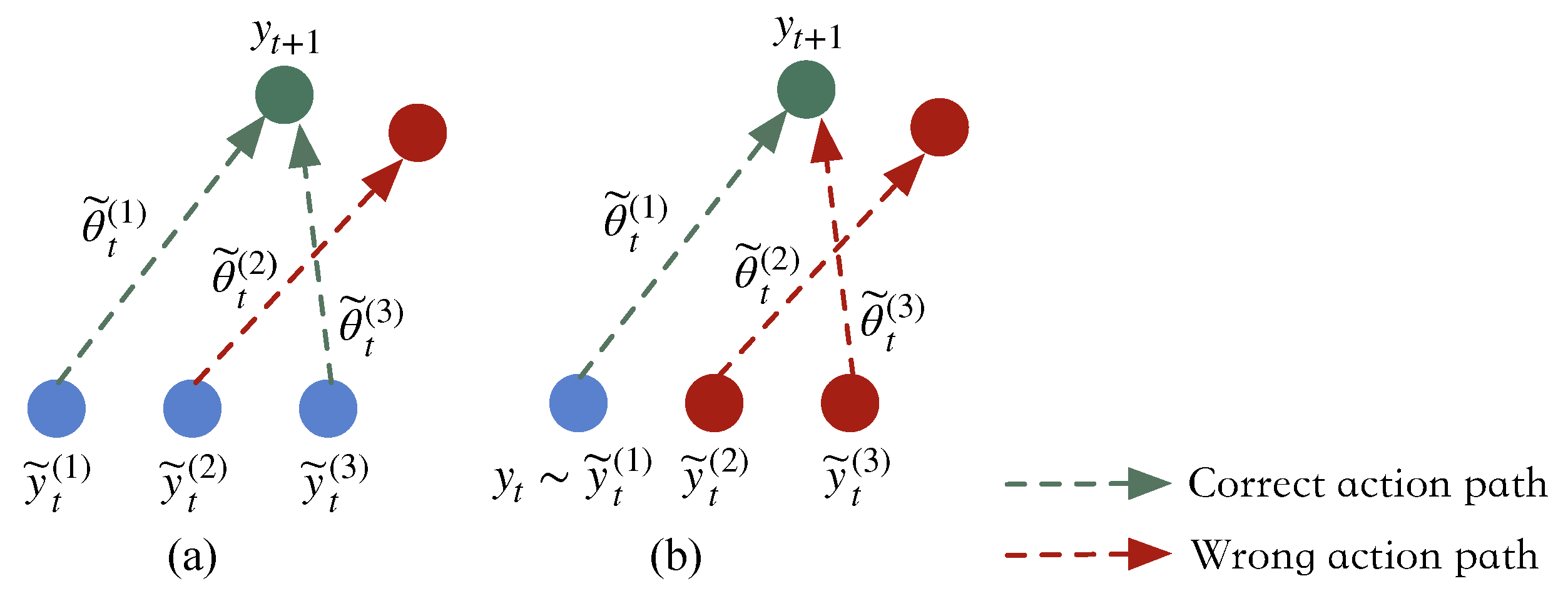
However, the primary goal of the existing observation–tracking problem is to accurately track the observation vector $\mathit{y}$ at a specific time slice, which ignores the consistency of the observation transition across consecutive time slices in the entire trajectory and thereby decreases the accuracy and stability of the hidden parameters $\mathit{\theta }$. An example of the observation–tracking problem is shown in Figure 1a. In the process of observation tracking, the estimated hidden parameter ${\tilde{\mathit{\theta }}}_t$ at time slice t will be acceptable as long as the single point of the observation ${\mathit{y}}_{t+1}$ is accurately tracked. However, the estimated parameter ${\tilde{\mathit{\theta }}}_t$ is difficult to keep stable due to the constant struggle to ensure high-accuracy observation tracking. Therefore, this paper extends the observation–tracking problem to an observation–trajectory alignment problem to overcome the aforementioned limitation and incorporate additional considerations into the estimation goal.

The key principle for extending the problem definition and maintaining stable hidden-parameter estimation is to constrain the accuracy of the observation trajectory rather than that of a single-point estimate. To achieve this principle, as illustrated in Figure 1b, in the observation–trajectory alignment problem, the observation tracking errors at the start and end points of the trajectory are both considered to help reduce the risk that a wrong tracked observation at the previous time slice will increase the estimation fluctuation of hidden parameters. The estimation goal based on the observation–trajectory alignment problem can be extended as Equation (3):

$${\tilde{\mathit{\theta }}}_{t+1}=\min {\arg }_{\mathit{\theta }}(e_1+e_2+e_3)$$

(3)

$$e_1=\left|\right|{\mathit{y}}_{t+1}-F({\tilde{\mathit{y}}}_t,{\mathit{u}}_{t+1},{\mathit{\theta }}_t){\left|\right|}_1$$

(4)

$$e_2=\left|\right|{\mathit{y}}_{t+1}-F({\mathit{y}}_t,{\mathit{u}}_{t+1},{\mathit{\theta }}_t){\left|\right|}_1$$

(5)

$$e_3=\left|\right|{\mathit{y}}_t-{\tilde{\mathit{y}}}_t{\left|\right|}_1$$

(6)

Compared with Equation (1), Equation (3) considers joint tracking errors at multiple time slices to represent the alignment error of the observation trajectory. Specifically, $e_1$, as shown in Equation (4), represents the tracking error from the previous estimated observation ${\tilde{y}}_t$. As shown in Equation (5), $e_2$ represents the tracking error from the ground truth observation $y_t$ to reduce the impact from large tracking deviations of the previous observation on the hidden-parameter estimation. Finally, $e_3$, which is shown in Equation (6), represents the tracking error of observations at the previous time slice to align the start point of the observation trajectory and ensure the stability of estimated hidden parameters.

3. Methodology of Parameter Estimation Based on LAC-T Framework

3.1. Overview of the LAC-T Framework

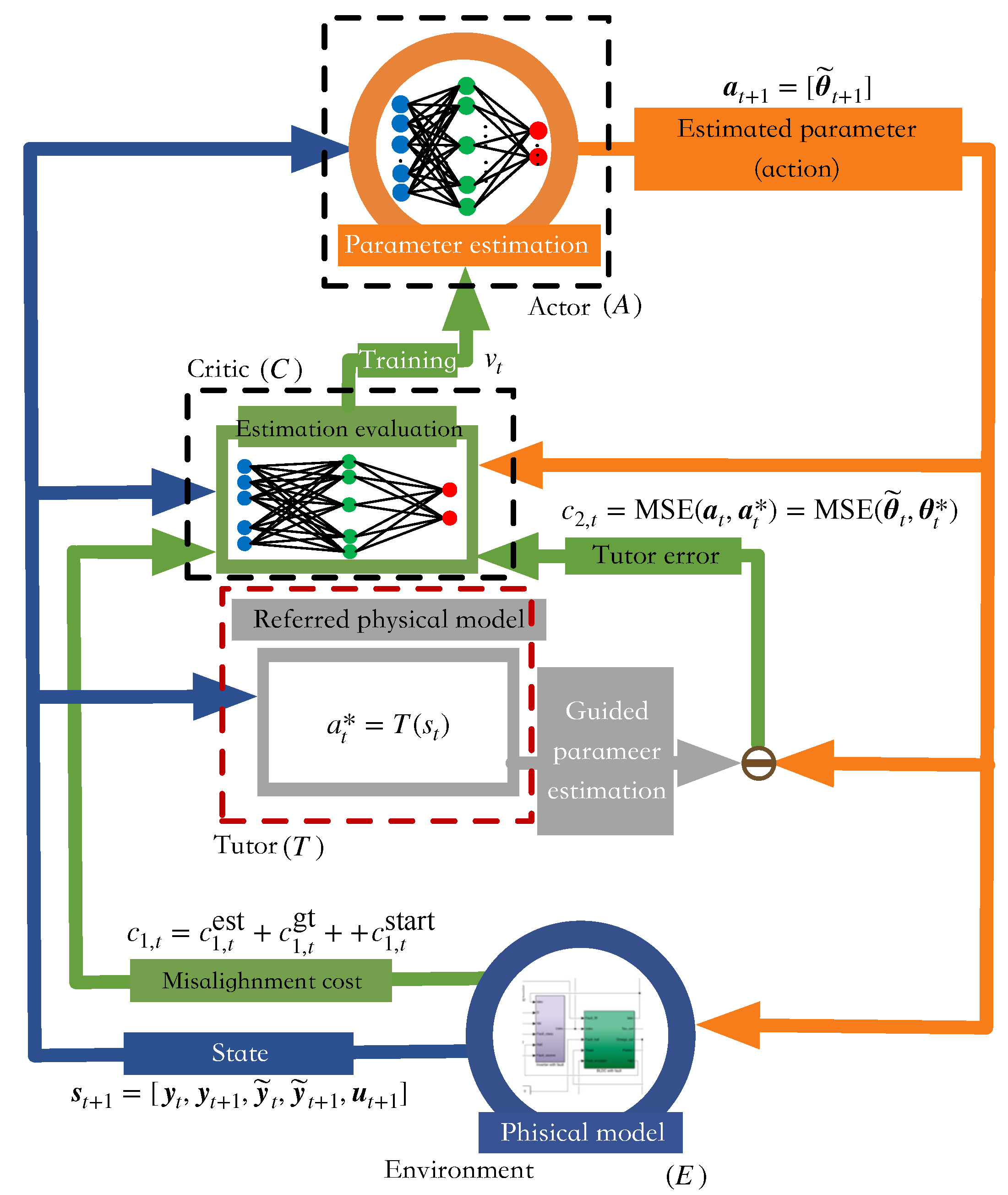
Based on the problem definition for hidden-parameter estimation, a Lyapunov Actor–Critic Tutor (LAC-T) framework is proposed. As illustrated in Figure 2, the proposed LAC-T framework consists of four components: Environment, Actor, Critic, and Tutor. In detail, the environment component is constructed from rotating systems based on state-system principles that describe the mapping between the input, hidden parameters and observations. The actor component is used to estimate hidden parameters to reflect the hidden health status of rotating systems. The critic component evaluates the correctness of the estimated hidden parameters and helps train the actor component. The basic principle of the actor, environment and critic components is described in Equations (7)–(9).

$${\mathit{a}}_t=A\left({\mathit{s}}_t\right)\sim {\pi }_A\left({\mathit{a}}_t\right|{\mathit{s}}_t)$$

(7)

$$[{\mathit{s}}_t,r_t]=E({\mathit{s}}_t,{\mathit{a}}_t)$$

(8)

$$v_t=C({\mathit{a}}_t,{\mathit{s}}_t)=L_C({\mathit{a}}_t,{\mathit{s}}_t)$$

(9)

where A, E, C, and T represent map functions of the actor, environment, critic, and tutor components, respectively. ${\mathit{a}}_t$ and ${\mathit{s}}_t$ represent the action vector and state vector in the reinforcement learning framework at time slice t. $r_t$ represents the reward provided by the environment component, and $v_t$ is the evaluation from the critic component at time slice t.

From a mathematical perspective, hidden-parameter estimation can be viewed as an equation-solving problem, in which the hidden parameters are treated as dependent variables and the observations as independent variables. However, due to the nonlinear nature of complex rotating systems, the mapping from hidden parameters to observations can admit multiple solutions. Therefore, multiple solutions yield multiple numerical directions that satisfy the requirements of observation tracking but violate the physical principle in rotating systems. To avoid the anti-physical multiple solutions in existing hidden-parameter estimation methods, the proposed framework introduces a tutor component to provide reference directions for the actor component, thereby improving the accuracy of hidden-parameter estimation, whose basic principle is described in Equation (10).

$${\mathit{a}}_t^{*}=T\left({\mathit{s}}_t\right)$$

(10)

It is worth noting that the tutor component can be generated either from a pre-trained data-driven model or from a simplified physical model informed by expert knowledge. In the LAC-T framework, the reference from the tutor component ${\mathit{a}}_t^{*}$ is used to release the struggle of the multiple solutions and guide the estimation process of the actor component toward the right direction, and thus improve the accuracy of hidden-parameter estimation.

3.2. Design of RL Elements in the LAC-T Framework

To estimate the hidden parameters of rotating systems using the LAC-T framework, it is necessary to specify the state space $\mathit{s}$, the action space $\mathit{a}$ and the reward r. According to the problem definition in Section 2, hidden-parameter estimation can be viewed as an observation–trajectory alignment problem. Therefore, the actor component needs to consider the observation’s ground truth and its estimation simultaneously across multiple time slices. Therefore, the state space at time slice $t+1$ in the LAC-T framework is described in Equation (11)

$${\mathit{s}}_{t+1}=[{\mathit{y}}_t,{\mathit{y}}_{t+1},{\tilde{\mathit{y}}}_t,{\tilde{\mathit{y}}}_{t+1},{\mathit{u}}_{t+1}]$$

(11)

where ${\mathit{y}}_t$ and ${\tilde{\mathit{y}}}_t$ represent the observation’s ground truth and estimation at time slice t. Similarly, ${\mathit{y}}_{t+1}$ and ${\tilde{\mathit{y}}}_{t+1}$ represent the observation’s ground truth and estimation at time slice $t+1$. ${\mathit{u}}_{t+1}$ is the input in the LAC-T framework at time slice $t+1$.

Under the background of hidden-parameter estimation, the action space generated by the actor component corresponds to the estimated hidden parameter $\mathit{\theta }$ and drives the environment component to generate the state in the next time slice. Therefore, the action space is designed as Equation (12):

$${\mathit{a}}_{t+1}=\left[{\tilde{\mathit{\theta }}}_{t+1}\right]$$

(12)

where ${\tilde{\mathit{\theta }}}_{t+1}$ represents the estimated hidden parameters at time slice $t+1$.

Except for the action and state spaces, the cost function, which could be specified as the negative of the reward and described as $c_t=-r_t$, also needs a specific design. Based on the background of hidden-parameter estimation and the proposed LAC-T framework, the cost can be divided into two parts, as listed in

Table 1. Cost formulation in the proposed LAC-T framework.

Component	Mathematical Expression	Function Description
Estimated trajectory alignment cost	$c_{1,t}^{\mathrm{est}}={∥{\mathit{y}}_{t+1}-F({\tilde{\mathit{y}}}_t,{\mathit{u}}_{t+1},{\tilde{\mathit{\theta }}}_t)∥}_1$	Constrains the transition trajectory from the estimated observation
Ground-truth trajectory alignment cost	$c_{1,t}^{\mathrm{gt}}={∥{\mathit{y}}_{t+1}-F({\mathit{y}}_t,{\mathit{u}}_{t+1},{\tilde{\mathit{\theta }}}_t)∥}_1$	Constrains the transition trajectory from the true observation
Start-point alignment cost	$c_{1,t}^{\mathrm{start}}={∥{\mathit{y}}_t-{\tilde{\mathit{y}}}_t∥}_1$	Aligns the starting point of the observation trajectory
Observation–trajectory misalignment cost	$c_{1,t}=c_{1,t}^{\mathrm{est}}+c_{1,t}^{\mathrm{gt}}+c_{1,t}^{\mathrm{start}}$	Observation trajectory-level alignment to keep the stability of the hidden-parameter estimation
Tutor-guided physical cost	$c_{2,t}=\mathrm{MSE}({\tilde{\mathit{\theta }}}_t,{\mathit{\theta }}_t^{*})$	Constrains the action toward the tutor-guided parameter
Integrated cost	$c_{r,t}=\mu c_{1,t}+(1-\mu )c_{2,t}$	Balances trajectory alignment and tutor guidance

.

The first cost comes from the observation–trajectory alignment error, which keeps the stability of hidden-parameter estimation. As described in Section 2, the LAC-T framework considers not only observation–tracking accuracy at a single time slice but also the consistency of the observation transition across consecutive time slices in the entire trajectory. Therefore, this part of the cost function is designed as shown in Equation (13):

$$\begin{array}{cc}\hfill c_{1,t}& =c_{1,t}^{\mathrm{est}}+c_{1,t}^{\mathrm{gt}}++c_{1,t}^{\mathrm{start}}\hfill \\ \hfill & =\underset{\mathrm{estimated}\mathrm{trajectory}\mathrm{alignment}}{\underbrace{{∥{\mathit{y}}_{t+1}-F({\mathit{y}}_t,{\mathit{u}}_{t+1},{\tilde{\mathit{\theta }}}_t)∥}_1}}+\underset{\mathrm{ground}\text{-}\mathrm{truth}\mathrm{trajectory}\mathrm{alignment}}{\underbrace{{∥{\mathit{y}}_{t+1}-F({\mathit{y}}_t,{\mathit{u}}_{t+1},{\tilde{\mathit{\theta }}}_t)∥}_1}}+\underset{\mathrm{start}\text{-}\mathrm{point}\mathrm{alignment}}{\underbrace{{∥{\mathit{y}}_t-{\tilde{\mathit{y}}}_t∥}_1}}\hfill \end{array}$$

(13)

Moreover, to ensure that hidden-parameter estimation is physically meaningful, the tutor and actor components estimate the hidden parameters synchronously, guiding the actor towards the correct ones. Therefore, the second part of the cost function is described in Equation (14):

$$c_{2,t}=\mathrm{MSE}({\mathit{a}}_t,{\mathit{a}}_t^{*})=\mathrm{MSE}({\tilde{\mathit{\theta }}}_t,{\mathit{\theta }}_t^{*})$$

(14)

where ${\tilde{\mathit{\theta }}}_t$ represents the estimated hidden parameter generated from the actor component at time slice t, while ${\mathit{\theta }}_t^{*}$ is the estimated hidden parameter from the tutor component. MSE is the mean squared error function between ${\tilde{\mathit{\theta }}}_t$ and ${\mathit{\theta }}_t^{*}$.

Combined with Equations (13) and (14), the integrated cost function is calculated as Equation (15):

$$c_{r,t}=\mu c_{1,t}+(1-\mu )c_{2,t}$$

(15)

where $\mu$ is set as the weight to balance the contribution of $c_{1,t}$ and $c_{2,t}$ in the training process. $c_{r,t}$ represents the integrated cost as the input of the Lyapunov critic component, which guides the actor component to estimate hidden parameters with a limited range and improves the accuracy of hidden-parameter estimation.

3.3. The Learning Strategy of Hidden-Parameter Estimation Based on LAC-T

Based on the LAC-T framework’s structure with a specific action space, state space and cost function, the learning strategy also need to be specific. Inspired by [38], the actor is updated by minimising the following Lyapunov-constrained objective described in Equation (16):

$$\begin{array}{cc}\hfill J\left(A\right)=& E_D\left[\beta \left[\log A\left({\mathit{s}}_t\right)\right]\right]+\hfill \\ \hfill & \lambda (L_{C,{\mathsf{\Phi }}_L}({\mathit{s}}_{t+1},A\left({\mathit{s}}_{t+1}\right))-L_{C,{\mathsf{\Phi }}_L}({\mathit{s}}_t,A\left({\mathit{s}}_t\right))+{\alpha }_3{c}_t)+\hfill \\ \hfill & \alpha \left|\right|A^{*}\left({\mathit{s}}_t\right)-A^{*}\left({\mathit{s}}_{near}\right)\left|\right|\hfill \end{array}$$

(16)

where $\beta$ represents the entropy regularisation coefficient that controls the importance of the stability guarantee. $\lambda$ represents the positive Lagrange multiplier for the Lyapunov constraint. ${\alpha }_3$ represents the Lyapunov decreasing margin coefficient. $\alpha$ represents the policy smoothness regularisation coefficient. ${\mathit{s}}_{near}$ represent a near state to state ${\mathit{s}}_{\mathit{t}}$.

The objective function for actor updating comprises three parts. The first term $E_D\left[\beta \left[\log A\left({\mathit{s}}_t\right)\right]\right]$ is the policy entropy regularisation term, which is used to enhance the stochasticity and exploration capability of the policy. It prevents the policy from prematurely converging to a suboptimal solution, thereby improving the stability and robustness of the training process. The second term $\lambda (L_{C,{\mathsf{\Phi }}_L}({\mathit{s}}_{t+1},A\left({\mathit{s}}_{t+1}\right))-L_{C,{\mathsf{\Phi }}_L}({\mathit{s}}_t,A\left({\mathit{s}}_t\right))+{\alpha }_3{c}_t)$ is the stability constraint term based on the Lyapunov function. Its main purpose is to ensure that the policy satisfies the system’s stability requirement while optimising the actor’s performance. Specifically, $L_{C,{\mathsf{\Phi }}_L}({\mathit{s}}_{t+1},A\left({\mathit{s}}_{t+1}\right))-L_{C,{\mathsf{\Phi }}_L}({\mathit{s}}_t,A\left({\mathit{s}}_t\right))$ describes the variation of the Lyapunov function during the system state transition, while ${\alpha }_3{c}_t$ provides a cost-related decreasing margin. Therefore, this term constrains the actor to learn actions that are not only effective but also capable of driving the system toward a more stable and safer direction. The third term $\left|\right|A^{*}\left({\mathit{s}}_t\right)-A^{*}\left({\mathit{s}}_{near}\right)\left|\right|$ is a smoothness regularisation term, which is introduced to constrain the difference between the actions generated under neighbouring states. This term reduces the policy’s sensitivity to local perturbations, making the actor-learned hidden-parameter estimation policy smoother and more continuous while also improving its generalisation capability. These three components guide the actor’s training from the perspectives of exploration, stability, and continuity, respectively. As a result, the learned policy can simultaneously account for performance optimisation, safety constraints, and practical implementability.

In the proposed LAC-T framework, the Lyapunov critic $L_C({\mathit{s}}_t,{\mathit{a}}_t)$ is introduced to impose a stability-oriented constraint on the actor update. Specifically, the Lyapunov term encourages the learned policy to generate hidden-parameter estimates such that the Lyapunov value decreases along the sampled estimation trajectory. However, this stability guarantee should be interpreted as local rather than global. The reason is that the state vector ${\mathit{s}}_t=[{\mathit{y}}_{t-1},{\mathit{y}}_t,{\tilde{\mathit{y}}}_{t-1},{\tilde{\mathit{y}}}_t,{\mathit{u}}_t]$, the action ${\mathit{a}}_t=\left[{\tilde{\mathit{\theta }}}_t\right]$, and the tutor-guided action $a_t^{*}=\left[{\mathit{\theta }}_t^{*}\right]$ are all defined within the physically admissible operating region of the rotating system. Moreover, the Lyapunov critic and the actor policy are learned from sampled data within the replay buffer, rather than being analytically verified over the entire state-action space. Therefore, the Lyapunov decrease condition is expected to hold within the bounded region defined by the training data, degradation scenarios, and admissible range of hidden parameters. Under ideal conditions where the learned Lyapunov function is exact and the decrease condition is strictly satisfied, the estimation error can be regarded as locally asymptotically stable. In practical cases with neural approximation errors, tutor bias, and observation noise, the stability implication is more appropriately interpreted as local uniform ultimate boundedness. Consequently, the proposed LAC-T framework does not claim global asymptotic stability; instead, the Lyapunov function locally enhances the stability of hidden-parameter estimation within the bounded region of attraction considered in this paper.

Based on the objective function and the training process of LAC-T, the major hyperparameters and their sensitivity to model convergence are listed in

Table 2. Hyperparameters of the LAC-T framework.

Symbol	Name	Sensitivity to Model Convergence
$l{r}_A$	Actor learning rate	High. A large value may cause unstable policy updates or divergence, whereas a small value may lead to slow convergence and poor optimization efficiency.
$l{r}_L$	Lyapunov critic learning rate	High. An inappropriate value may lead to inaccurate Lyapunov estimation, weakening the stability constraint and affecting the actor’s convergence.
$\gamma$	Discount factor	Medium. A large value emphasises long-term performance but may increase training difficulty, while a small value may ignore long-term degradation or stability trends.
$\beta$	Entropy regularisation coefficient	Medium. A large value may make the policy overly random and slow down convergence, whereas a small value may reduce exploration and cause premature convergence.
$\lambda$	Lagrange multiplier for Lyapunov constraint	High. A large value may make the policy overly conservative, while a small value may fail to enforce the stability constraint, leading to unsafe or unstable learning.
${\alpha }_3$	Lyapunov decrease margin coefficient	High. A large value imposes a strict Lyapunov decrease condition and may make optimisation difficult, whereas a small value may weaken the stability guarantee.
$\alpha$	Policy smoothness regularisation coefficient	Medium. A large value may overly restrict policy flexibility, while a small value may fail to suppress sensitivity to local perturbations.

. These hyperparameters govern both the learning dynamics and the stability-aware policy optimisation process. The actor learning rate $l{r}_A$ determines the magnitude of policy updates, thereby affecting how quickly the control policy can adapt to sampled transitions. Meanwhile, the Lyapunov critic learning rate $l{r}_L$ is associated with the Lyapunov function’s approximation accuracy and training efficiency, providing a basis for evaluating the learned policy’s tendency toward stability. The discount factor $\gamma$ controls the trade-off between immediate and future rewards or costs, making it particularly important for capturing long-term degradation trends and stability-related consequences. To maintain sufficient exploration during policy learning, the entropy coefficient $\beta$ is introduced to regulate the randomness of the policy distribution and reduce the risk of being trapped in local optima. In addition, the Lagrange multiplier $\lambda$ adjusts the relative importance of the Lyapunov constraint in the optimisation objective, thus balancing performance improvement with stability preservation. The coefficient ${\alpha }_3$ further determines the required decrease margin of the Lyapunov function by scaling the instantaneous cost, which directly affects the strictness of the stability condition. Finally, the smoothness coefficient $\alpha$ imposes a regularisation effect on the policy outputs for neighbouring states, helping to suppress abrupt variations in action and enhance the robustness of the learned policy. Specifically, following the training strategy of the [38,39], $\beta$ and $\lambda$ can be adjusted through the gradient method by maximising the objective described in Equations (17) and (18):

$$J\left(\beta \right)=\beta {\mathbb{E}}_{\mathcal{D}}\left[\log \left(A\left({\mathit{s}}_t\right)\right)+{\mathcal{H}}_t\right]$$

(17)

$$J\left(\lambda \right)=\lambda (L_{C,{\mathsf{\Phi }}_L}({\mathit{s}}_{t+1},A\left({\mathit{s}}_{t+1}\right))-L_{C,{\mathsf{\Phi }}_L}({\mathit{s}}_t,A\left({\mathit{s}}_t\right))+{\alpha }_3{c}_t)$$

(18)

According to the designed reward and learning strategy, the training process of the LAC-T framework is described in Algorithm 1.

Algorithm 1 The training process of the LAC-T framework.

Require: Learning rate $l{r}_A$ and $l{r}_C$, environment component E, tutor component T Ensure: The trained actor component A    1:  Initialise Lyapunov network $L_{C,\mathsf{\Phi }}$ and strategy ${\pi }_A$ randomly    2:  Sample the initial state vector ${\mathit{s}}_0$    3:  while$\mathrm{epoch}>0$do    4:      while $t>0$ do    5:          Estimate hidden parameter ${\mathit{\theta }}_t$ as an action ${\mathit{a}}_t$ based on ${\pi }_A$ of actor component;    6:          Achieve the tutored parameter estimation ${\mathit{\theta }}_t^{*}$ as the tutored action ${\mathit{a}}_t^{*}$ based on tutor component;    7:          Input the observation $Y=\{{\mathit{y}}_{t-n},{\mathit{y}}_{t-n+1},\dots ,{\mathit{y}}_T\}$ into the E and achieve the estimated observation and loss function $c_{1,t}$;    8:          Compare the estimated hidden parameter ${\mathit{\theta }}_t$ with tutored hidden parameter ${\mathit{\theta }}_t^{*}$ to obtain the loss function $c_{2,t}$;    9:          Calculate the integrated loss $c_{r,t}$ based on $c_{1,t}$ and $c_{2,t}$;  10:          Compose $({\mathit{s}}_t,{\mathit{a}}_t,{\mathit{a}}_t^{*},c_{r,t},{\mathit{s}}_{t+1})$ and store it in the data pool D  11:      end while  12:      while $\mathrm{step}>0$ do  13:          Sample path from data pool D  14:          Update $L_{C,\mathsf{\Phi }}$ and ${\pi }_A$ using sampled path  15:          Update the target networks with soft replacement ${\overline{\varphi }}_L\leftarrow \tau {\varphi }_L+(1-\tau ){\overline{\varphi }}_L$  16:      end while  17:  end while

4. Experiment and Discussion

4.1. Experiment Setup

To validate the effectiveness and superiority of the proposed LAC-T framework for hidden-parameter estimation in health status monitoring, a case study of a high-speed rotor system from a control moment gyroscope (CMG), which is a typical rotating system in CMG, is conducted to evaluate the estimation accuracy and compare it with other candidate models. In the high-speed rotor system, the mechanical failure is generally caused by the degradation of the motor torque coefficient and can be reflected in the motor current and rotational speed [40], which can be observed by sensors. Therefore, to monitor the hidden degradation caused by mechanical failure and support potential maintenance of the high-speed rotor system, the motor torque coefficient is treated as a key hidden parameter and estimated from motor current and rotational speed time series.

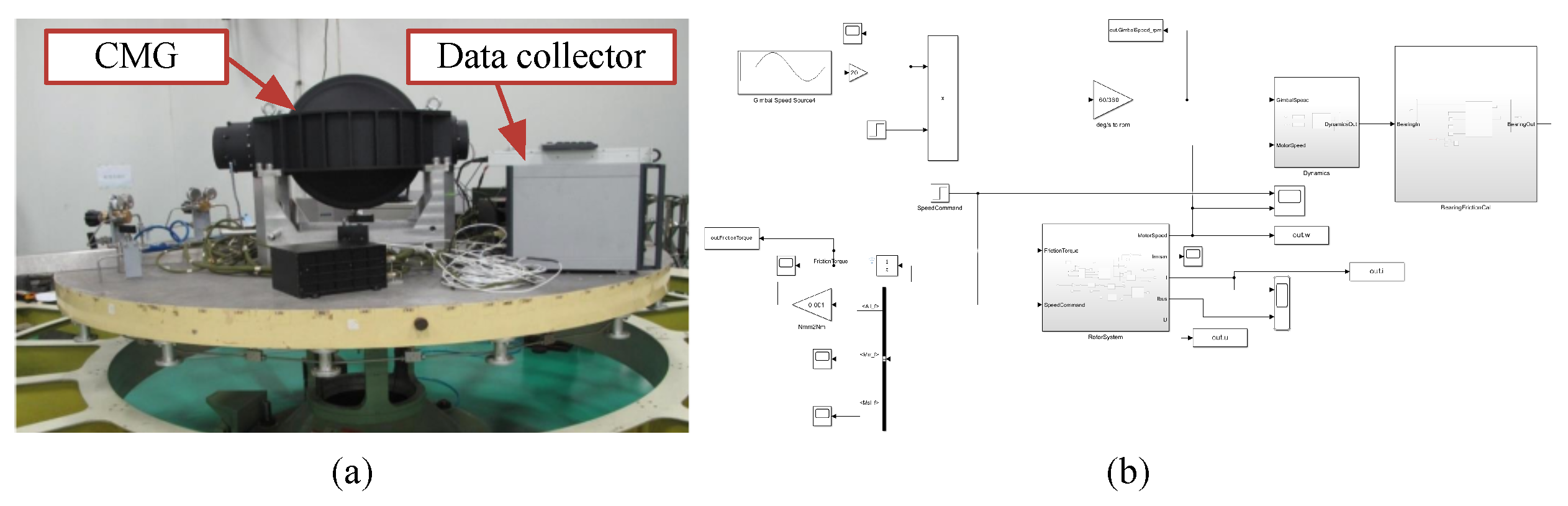
Based on the background of the case, to quantify the error of the estimated value of hidden parameters with the ground truth, and support the performance validation of the proposed LAC-T framework under various scenarios, the degradation value of the motor torque coefficient and corresponding observed value of the motor current and rotational speed are generated from a digital twin-driven degradation model, which has been established and validated by the previous work [21]. The experimental device of CMG and the corresponding digital twin-driven degradation model are shown in Figure 3.

To validate the effectiveness and superiority of the proposed LAC-T under various scenarios, different degradation modes are generated by the digital twin-driven model under the unified principle of the motor torque coefficient [41], which is described in Equation (19):

$$K_t=C_1-a_1\times e^{b_{1}t}$$

(19)

where $K_t$ represents the motor torque coefficient. $C_1$, $a_1$, and $b_1$ are hyperparameters in the degradation principle. $C_1$ controls the initial value of the degradation, while $a_1$ and $b_1$ control the degradation speed. The start point, speed and the initial value of degradation can be adjusted by changing the hyperparameter to generate various scenarios. In this case, six datasets across different degradation modes are generated for validation by specific hyperparameters, as listed in

Table 3. Experiment setup of different degradation modes.

	${\mathit{C}}_1$	${\mathit{a}}_1$	${\mathit{b}}_1$
Dataset 1	1	1.50 $\times {10}^{-5}$	5.20 $\times {10}^{-5}$
Dataset 2	1	2.26 $\times {10}^{-5}$	$1.00\times {10}^{-1}$
Dataset 3	0.8	2.80 $\times {10}^{-14}$	3.00 $\times {10}^{-1}$
Dataset 4	1	1.00 $\times {10}^{-4}$	1.70 $\times {10}^{-1}$
Dataset 5	1	1.00 $\times {10}^{-4}$	4.20 $\times {10}^{-1}$
Dataset 6	1	6.18 $\times {10}^{-10}$	2.00 $\times {10}^{-1}$

.

In this case, the motor current and rotational speed are observed to estimate the motor torque coefficient. Meanwhile, a lower-order physical model is selected as the tutor component of the LAC-T framework that maps the motor current and rotational speed to the motor torque coefficient. In this case, the mapping relationship is described as follows:

$$K_t={\displaystyle \frac{J}{i_s}}{\displaystyle \frac{\mathrm{d}\omega }{\mathrm{d}t}}$$

(20)

where $K_t$ is the the motor torque coefficient. $i_s$ and $\omega$ are the motor current and rotational speed, respectively. J represents the moment of inertia, which is provided by the motor supplier. Equation (20) is used as the governing equation of the tutor component in this case study. This lower-order physical model is selected because it directly maps the available observations, i.e., motor current and rotational speed. It should be noted that the tutor component is not used as the final estimator in the proposed LAC-T framework but provides a physically consistent reference action to guide the actor component. Therefore, the reduced-order representation is sufficient to provide the main direction of estimation while keeping the tutor model compact. Although the simplification may introduce bias when the physical model is used in isolation, the actor and critic components in the LAC-T can further mitigate this bias through data-driven policy optimisation and observation–trajectory alignment. In addition, the simplified model relies solely on numerical differentiation and algebraic operations, avoiding the online solution of a complex high-order model and improving the computational efficiency of the tutor component during training.

To quantify the performance of the LAC-T framework, root mean squared error (RMSE), mean absolute error (MAE), and normalised root mean square error (NRMSE) are selected to compute the estimation error of the hidden parameter with ground truth, which are computed in Equations (21)–(23):

$$e_{\mathrm{RMSE}}=\sqrt{{\displaystyle \frac{1}{T}}\sum _{t=1}^T{({\tilde{x}}_t-x_t)}^2}$$

(21)

$$e_{\mathrm{MAE}}={\displaystyle \frac{1}{T}}{\displaystyle \sum _{t=1}^T}|{\tilde{x}}_t-x_t|$$

(22)

$$e_{\mathrm{NRMSE}}={\displaystyle \frac{e_{\mathrm{RMSE}}}{\frac{1}{T}{\sum }_{t=1}^T{x}_t}}$$

(23)

where $x_t$ represents the ground truth value of hidden parameters and ${\tilde{x}}_t$ is the estimated value.

This case study was conducted on a MacBook Pro platform equipped with an Apple M4 chip, 64 GB of unified memory, and a built-in 40-core GPU. The software environment was based on macOS, with Python 3.12.12 as the primary programming language and the relevant models implemented using the PyTorch 2.9.1 deep learning framework.

4.2. Effectiveness Validation of the LAC-T Framework

To fully validate the effectiveness and generalisation of the proposed LAC-T framework under various scenarios, this case investigated six datasets across different modes with varying start points and speed of degradation, as described in Section 4.1 and listed in Table 3.

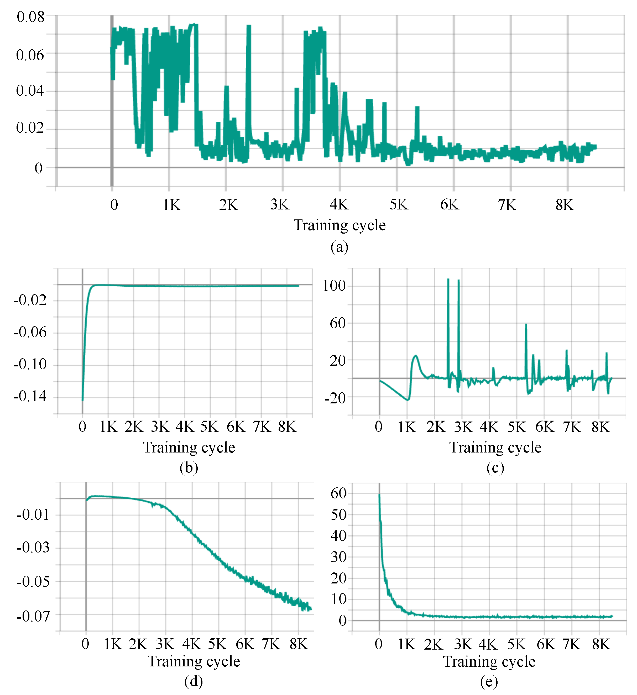
As shown in Figure 4, the loss function curve of the LAC-T framework reflects the effectiveness of framework learning and the improvement of the hidden-parameter estimation performance during the training process. In detail, the Lyapunov critic loss decreases and remains low during training, indicating that the critic component in the LAC-T framework effectively learns the stability-related evaluation function. Meanwhile, the actor loss converges to a stable range. This suggests that the actions generated by the actor component stabilise. During the training cycles from 3000 to 4000, the integrated reward-related cost, which is described in Equation (15), increases temporarily, indicating a short-term degradation in control performance. However, this increase is not accompanied by a noticeable deterioration in either the actor loss or the Lyapunov critic loss, suggesting that policy optimisation and the stability-related value function approximation remain generally stable during this stage. The Beta loss shows evident fluctuations over the same interval, implying that the adaptive regulation mechanism temporarily alters the policy distribution and increases cost. The Lambda loss changes with a persistent decreasing trend in the later training stage, indicating that the Lyapunov-based stability constraint remains effective and does not become unstable. Therefore, the temporary cost increase during the training cycles from 3000 to 4000 can be regarded as a transient performance fluctuation, mainly due to adaptive exploration or coefficient regulation. After this adjustment stage, the integrated reward-related cost decreases again and gradually converges to a low level. Overall, these loss curves demonstrate that the hidden-parameter estimation is stable and that the training process of the proposed LAC-T framework is effective.

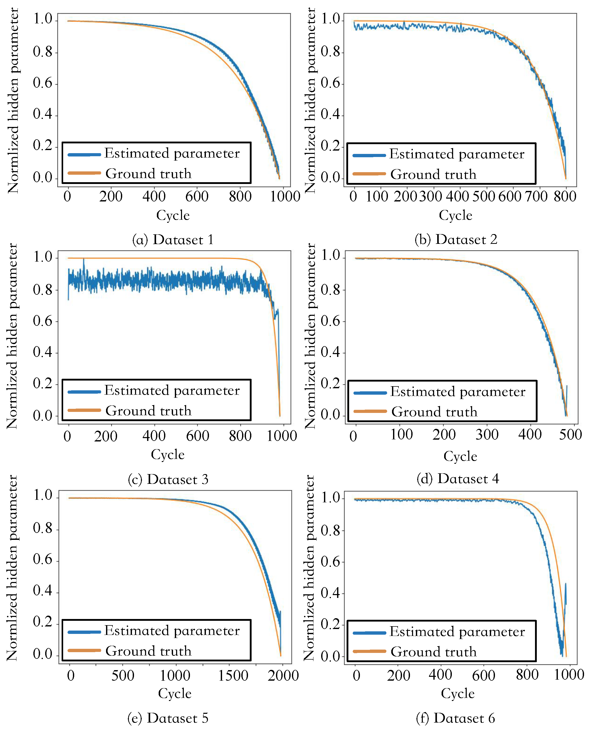
The experimental results of the motor torque coefficient estimation are shown in Figure 5 and

Table 4. The estimation error of the motor torque coefficient estimation using the LAC-T framework across various scenarios.

	${\mathit{e}}_{\mathbf{RMSE}}$	${\mathit{e}}_{\mathbf{MAE}}$	${\mathit{e}}_{\mathbf{NRMSE}}$
Dataset 1	0.12	0.07	0.13
Dataset 2	0.12	0.04	0.15
Dataset 3	0.31	0.16	0.48
Dataset 4	0.17	0.08	0.19
Dataset 5	0.31	0.19	0.31
Dataset 6	0.18	0.11	0.20

. The comparison between the estimated values and the ground truth in Figure 5 shows that the LAC-T framework can effectively estimate and track the change of the motor torque coefficient parameter across different value ranges and degradation speeds, especially at the degradation stage. The stable estimation error listed in Table 4 and the estimation curves at the motor torque coefficient degradation stage indicate the adaptive capacity of the proposed LAC-T framework across various scenarios with different degradation modes. Therefore, the experimental results for motor torque coefficient estimation demonstrate that the LAC-T framework proposed in this paper can effectively estimate hidden parameters to support health status monitoring of rotating systems.

4.3. Superiority Validation of the LAC-T Framework

To further demonstrate the superiority of the LAC-T framework for hidden-parameter estimation, two comparisons are investigated. Firstly, to demonstrate the superiority of the problem definition, this case compares hidden-parameter estimation errors of the LAC-T framework under the problem definition of the observation–tracking problem and the observation–trajectory alignment problem, respectively, by varying the reward defined in Equations (1) and (3). Secondly, to demonstrate the superiority of the LAC-T framework, especially the added tutor component, this case compares the physical model and the existing LAC model, a data-driven method, in their performance in the motor torque coefficient estimation.

In the first comparison, based on the definition of the observation–tracking problem and the observation–trajectory alignment problem, rewards are changed during the training process of the LAC-T framework. To quantify estimation stability under both problems, second-difference roughness (SDR) [42] is used to measure the oscillation of the estimated series of the motor torque coefficient, which is calculated in Equation (24).

$$R_{{\Delta }^2}={\displaystyle \sum _{t=2}^{T-1}}{(e_{t+1}-2e_t+e_{t-1})}^2$$

(24)

$$e_t={\tilde{x}}_t-x_t$$

(25)

where $e_t$ represents the estimation error at time slice t, in which $x_t$ represents the ground truth value and ${\tilde{x}}_t$ is the estimated value of the motor torque coefficient.

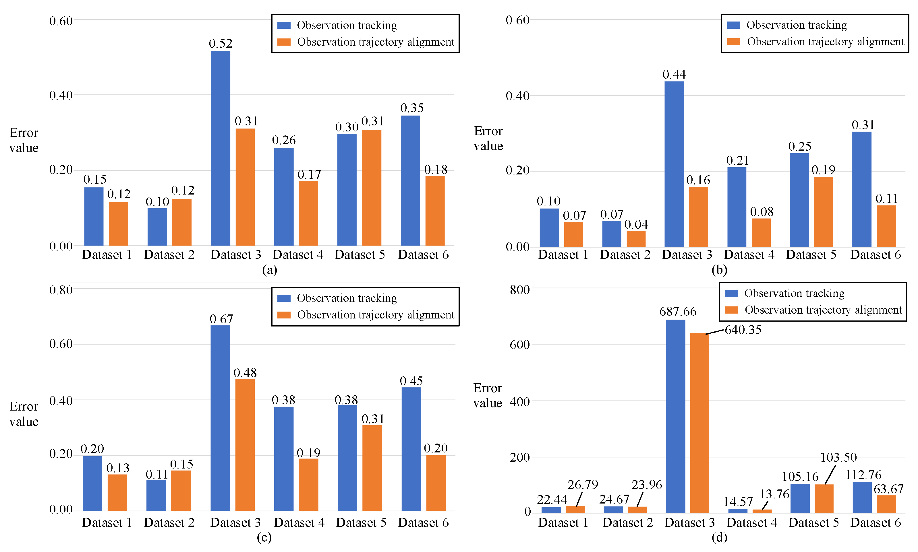
The experimental results are shown in Figure 6 and

Table 5. Mean estimation errors of motor torque coefficient under various problem definitions.

	${\mathit{e}}_{\mathbf{RMSE}}$	${\mathit{e}}_{\mathbf{MAE}}$	${\mathit{e}}_{\mathbf{NRMSE}}$	${\mathit{R}}_{{\Delta }^2}$
Observation tracking	0.28	0.23	0.36	161.21
Observation trajectory alignment	0.20	0.11	0.24	145.34

. As listed in Table 5 and Figure 6d, the observation–trajectory alignment problem definition shows greater stability than that under the observation–tracking problem definition, with a lower SDR value. Meanwhile, the RMSE, MAE, and NRMSE, as listed in Table 5 and Figure 6a–c, show that estimation errors under the observation–trajectory alignment problem are lower than those under the observation–tracking problem. These experimental results indicate that the estimation accuracy of hidden parameters is also improved when the observation trajectory is aligned by considering the tracked observation at both the start and end points along with the ground truth, which constrains the value range of hidden parameters.

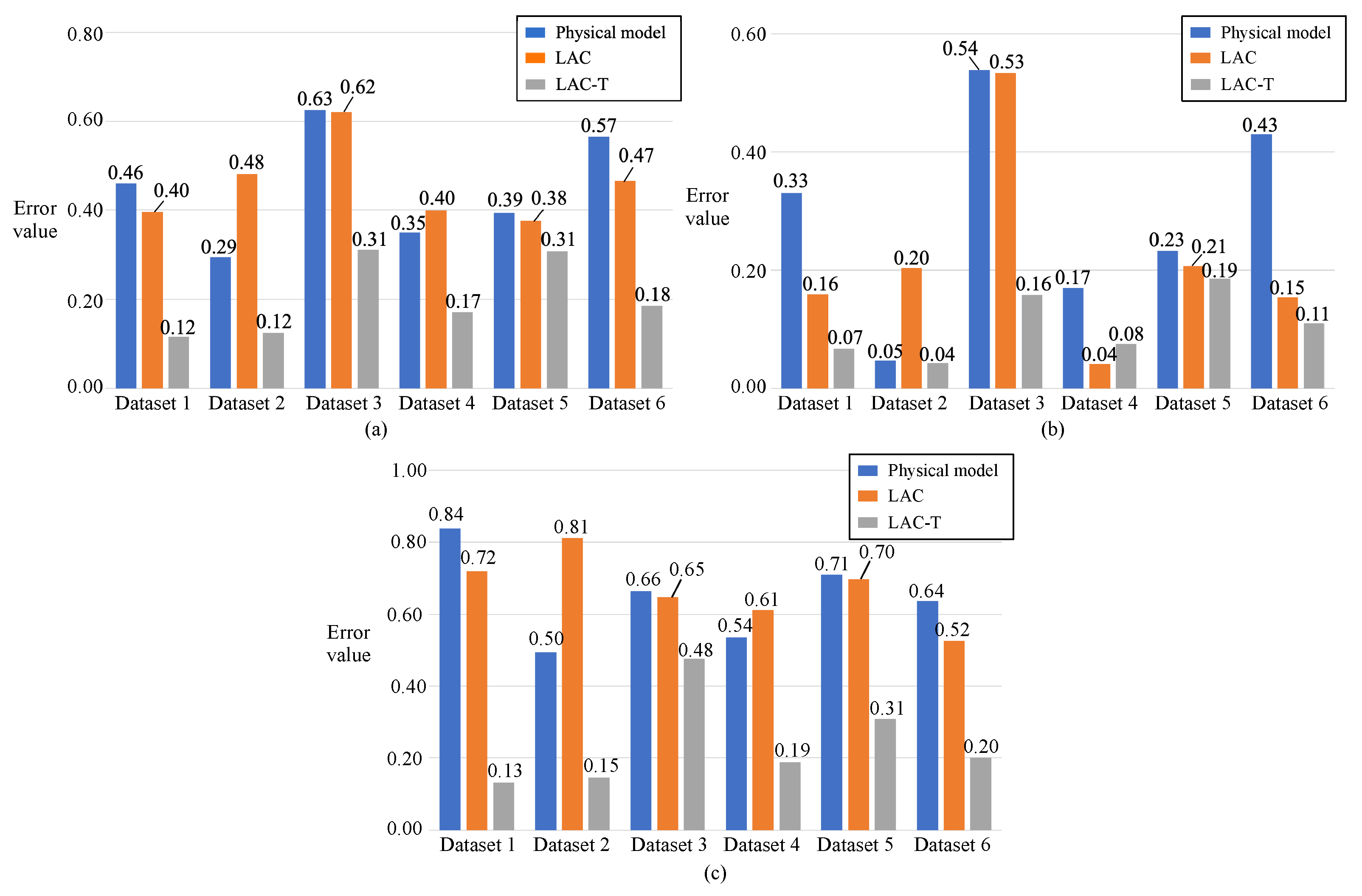
In the second comparison, to assess the superiority of the LAC-T framework, especially the added tutor component, the physical model and LAC, which is a data-driven reinforcement learning framework, are selected as candidate methods for motor torque coefficient estimation. As shown in

Table 6. Mean estimation errors of motor torque coefficient with different methods.

	${\mathit{e}}_{\mathbf{RMSE}}$	${\mathit{e}}_{\mathbf{MAE}}$	${\mathit{e}}_{\mathbf{NRMSE}}$
Physical model	0.45	0.29	0.65
LAC	0.46	0.22	0.67
LAC-T	0.20	0.11	0.24

, the estimation error of the physical model is slightly lower than that of LAC, indicating that incorporating human knowledge of the physical principle can improve estimation accuracy compared with a pure data-driven method. Furthermore, compared with the physical model and LAC, the LAC-T obtains a much lower estimation error. This shows that when a tutor component is introduced into the data-driven method, which combines the physical principle with data training, the estimated hidden parameters try to fit the guided ${\theta }^{*}$. In other words, the accuracy of hidden-parameter estimation is improved by leveraging additional physical information. Figure 7 also shows that the advantage of LAC-T is general, reflected by lower estimation error in various scenarios under different degradation modes.

To compare the estimated performance of the combination of the problem definition and proposed tutor component, a cross-combination ablation study is conducted, whose mean estimation errors are listed in

Table 7. Mean estimation errors of motor torque coefficient under various problem definitions and with/without the tutor component.

	${\mathit{e}}_{\mathbf{RMSE}}$	${\mathit{e}}_{\mathbf{MAE}}$	${\mathit{e}}_{\mathbf{NRMSE}}$	${\mathit{R}}_{{\mathbf{\Delta }}^2}$
LAC with observation tracking	0.62	0.57	0.80	181.52
LAC with observation trajectory alignment	0.46	0.22	0.67	157.57
LAC-T with observation tracking	0.28	0.23	0.36	161.21
LAC-T with observation trajectory alignment	0.20	0.11	0.24	145.34

. In this comparison, the problem definition (observation–tracking and observation–trajectory alignment) and LAC with/without the tutor component are jointly investigated. From the experimental results listed in Table 7, the estimation errors, especially the RMSE, MAE and NRMSE, of the LAC are higher than those of the LAC-T, demonstrating that the added tutor increases estimation accuracy. Meanwhile, in both the LAC and LAC-T frameworks, the $R_{{\Delta }^2}$ of observation tracking is higher than that of observation trajectory alignment, indicating that the problem definition of the observation trajectory alignment improves the stability of hidden-parameter estimation.

4.4. The Computation Cost Comparison of the LAC-T Framework

In addition to the estimation performance comparison of the proposed LAC-T framework, this case also investigated its computational cost. Considering the measures of inference efficiency and time consumption in the hidden-parameter estimation process, three indicators are selected to quantify estimation performance: single-sample inference latency per 10,000 steps, throughput and end-to-end latency. First, the comparison results for various problem definitions and with/without the tutor component are presented in

Table 8. The computational resource cost used by various problem definitions and the RL framework.

	Single-Sample Inference Latency per 10,000 Steps	Throughput	End-to-End Latency
LAC with observation–tracking	1.31	7449.57	227.83
LAC with observation–trajectory alignment	1.32	7442.53	228.11
LAC-T with observation–tracking	1.30	7501.37	226.76
LAC-T with observation–trajectory alignment	1.33	7349.85	232.03

. In the experimental results, the end-to-end latency of the LAC-T with observation trajectory alignment is the lowest, while its end-to-end latency is the highest, indicating that the introduction of the tutor component and the additional costs indeed increase computational cost.

This case also compared the computation cost of the LAC-T framework with other action constraint strategies that ensure the stability of hidden-parameter estimation, including the approaches that rely on control barrier functions (CBFs) or cost-shaped Lyapunov terms. The comparison results are listed in

Table 9. The computational resource cost under various stability strategies.

	Single-Sample Inference Latency per 10,000 Step	Throughput	End-to-End Latency
LAC with CBF	1.34	7308.33	231.86
LAC with cost-shaped Lyapunov terms	1.29	7684.55	219.98
LAC-T	1.33	7349.85	232.03

. The experimental results show that the LAC with cost-shaped Lyapunov terms consumes fewer computational costs than the LAC with CBF and the proposed LAC-T. Meanwhile, the end-to-end latency of the LAC with CBF and the proposed LAC-T are close, indicating that their computational complexity is nearly the same. However, the LAC-T has higher throughput than the LAC with CBF, indicating that it can process more samples per unit time, reflecting better batch inference efficiency and computational utilisation.

Finally, this case considers the influence of the framework dimension on the computational cost. In the efficiency and superiority validation experiment in this case, the actor is designed as a three-layer linear network with 64 dimensions. In this case, the framework dimension is changed from 4 to 512 to investigate computational cost usage across various actor-component dimensions. The comparison results are listed in

Table 10. The computational resource cost used by various system dimensions.

Actor Dimension	FLOPs	Single-Sample Inference Latency per 10,000 Steps	Throughput	End-to-End Latency
4	118	1.22	8041.07	214.54
8	362	1.22	8109.24	212.42
16	1234	1.22	8146.66	211.15
32	4514	1.22	8134.63	211.20
64	17,218	1.28	7741.00	218.39
128	67,202	1.28	7754.22	218.21
256	265,474	1.29	7685.21	219.85
512	1,055,234	1.34	7414.57	225.81

. It is noted that floating-point operations (FLOPs) are added to measure the model size. As shown in the experimental results, throughput decreases and end-to-end latency increases as actor-component dimensions increase, indicating that the computational cost increases with mode size.

5. Conclusions

Health status monitoring is critical for rotating systems to maintain safety and reliability. To address hidden-parameter estimation caused by the absence of critical sensors, this paper proposes an extended reinforcement learning framework named the Lyapunov Actor–Critic Tutor (LAC-T). In this framework, parameter estimation is redefined as an observation–trajectory alignment problem rather than an observation–tracking problem to maintain the stability of the estimated hidden parameters. Further, a tutor component is introduced into the framework to guide parameter estimation to address the multi-resolution problem. To validate the effectiveness and superiority of the proposed LAC-T framework, this paper presents a case study of motor torque coefficient estimation for a high-speed rotor system in a control moment gyroscope. The lower estimation error of the proposed LAC-T framework across six degradation modes demonstrates its effectiveness in hidden-parameter estimation across various scenarios. Meanwhile, the lower estimation error compared with the candidate problem definition and estimation methods indicates the superiority of the observation–trajectory alignment problem definition and the added tutor components. Finally, the computational cost comparison of the LAC-T framework is investigated. The lower throughput and higher end-to-end latency show that although the proposed LAC-T and the definition of the observation alignment problem can increase the accuracy and stability of hidden-parameter estimation, they do consume more computational cost when deployed. The LAC-T framework can be viewed as a hidden-state observer for rotating systems and utilised as a reference model to support fault detection and RUL prediction in complex systems. For future research directions, some challenges remain to be addressed. First, the robustness and accuracy of the tutor component are still critical factors affecting the performance of the LAC-T framework. How to ensure its consistency with practical tasks and maintain the stability of the overall LAC-T framework when the tutor component is inaccurate remains an important issue. Second, during deployment in real-world applications, the lightweight design of the LAC-T framework and improvements in its computational efficiency are important engineering considerations.

References

1. Park, Y.J.; Fan, S.K.S.; Hsu, C.Y. A Review on Fault Detection and Process Diagnostics in Industrial Processes. Processes 2020, 8, 1123. [Google Scholar] [CrossRef] [Scilit]
2. Zhou, J.; Yang, J.; Xiang, S.; Qin, Y. Remaining Useful Life Prediction Methodologies with Health Indicator Dependence for Rotating Machinery: A Comprehensive Review. IEEE Trans. Instrum. Meas. 2025, 74, 3528519. [Google Scholar] [CrossRef] [Scilit]
3. Habbouche, H.; Benkedjouh, T.; Amirat, Y.; Benbouzid, M. Rotating machine bearing health prognosis using a data driven approach based on KS-density and BiLSTM. IET Sci. Meas. Technol. 2025, 19, e12215. [Google Scholar] [CrossRef] [Scilit]
4. Wang, X.; Xie, D.; Li, Y.; Tian, J.; Li, K. Extended fault-pair Boolean table based test points selection for robotic systems. Intell. Robot. 2025, 5, 419–432. [Google Scholar] [CrossRef] [Scilit]
5. Kumar, S.; Raj, K.K.; Cirrincione, M.; Cirrincione, G.; Franzitta, V.; Kumar, R.R. A Comprehensive Review of Remaining Useful Life Estimation Approaches for Rotating Machinery. Energies 2024, 17, 5538. [Google Scholar] [CrossRef] [Scilit]
6. Shang, J.; Xu, D.; Li, M.; Qiu, H.; Jiang, C.; Gao, L. Remaining useful life prediction of rotating equipment under multiple operating conditions via multi-source adversarial distillation domain adaptation. Reliab. Eng. Syst. Saf. 2025, 256, 110769. [Google Scholar] [CrossRef] [Scilit]
7. Frost, S.; Goebel, K.; Celaya, J. A Briefing on Metrics and Risks for Autonomous Decision-making in Aerospace Applications. In Proceedings of the Infotech@Aerospace, Garden Grove, CA, USA, 19–21 June 2012. [Google Scholar] [CrossRef] [Scilit]
8. Qifeng, Y.; Longsheng, C.; Naeem, M.T. Hidden Markov Models based intelligent health assessment and fault diagnosis of rolling element bearings. PLoS ONE 2024, 19, e0297513. [Google Scholar] [CrossRef] [Scilit]
9. Yan, S.; Liu, H.; Li, F.; Huang, F.; Cui, H. An Integrated Condition Monitoring Method for Rotating Machinery Based on Optimum Healthy State. Machines 2022, 10, 1025. [Google Scholar] [CrossRef] [Scilit]
10. Sun, Z.; Wang, Y.; Zhang, L. Rotating machinery health state assessment under multi-working conditions based on a deep fuzzy clustering network. Measurement 2023, 218, 113172. [Google Scholar] [CrossRef] [Scilit]
11. Li, N.; Lei, Y.; Gebraeel, N.; Wang, Z.; Cai, X.; Xu, P.; Wang, B. Multi-Sensor Data-Driven Remaining Useful Life Prediction of Semi-Observable Systems. IEEE Trans. Ind. Electron. 2021, 68, 11482–11491. [Google Scholar] [CrossRef] [Scilit]
12. Huang, Z.; Shao, J.; Guo, W.; Li, W.; Zhu, J.; He, Q.; Fang, D. Tool Wear Prediction Based on Multi-Information Fusion and Genetic Algorithm-Optimized Gaussian Process Regression in Milling. IEEE Trans. Instrum. Meas. 2023, 72, 2516716. [Google Scholar] [CrossRef] [Scilit]
13. Xu, Z.; Zhang, B.; Luo Fan, L.; Hengzhou Yan, E.; Li, D.; Zhao, Z.; Sze Yip, W.; To, S. Deep-learning-driven intelligent tool wear identification of high-precision machining with multi-scale CNN-BiLSTM-GCN. Adv. Eng. Inform. 2025, 65, 103234. [Google Scholar] [CrossRef] [Scilit]
14. Alassery, F. Predictive maintenance for cyber physical systems using neural network based on deep soft sensor and industrial internet of things. Comput. Electr. Eng. 2022, 101, 108062. [Google Scholar] [CrossRef] [Scilit]
15. Zhang, D.; Hu, Y.; Zhang, S.; Zhang, Y. Distributed hierarchical reinforcement learning for dynamic maintenance scheduling of large-scale airline fleets. Reliab. Eng. Syst. Saf. 2026, 271, 112249. [Google Scholar] [CrossRef] [Scilit]
16. Wu, T.; Wang, L.; Xu, X.; Su, L.; He, W.; Wang, X. An intelligent fault detection algorithm for power transmission lines based on multi-scale fusion. Intell. Robot. 2025, 5, 474–487. [Google Scholar] [CrossRef] [Scilit]
17. Kulkarni, A.; Terpenny, J.; Prabhu, V. Sensor Selection Framework for Designing Fault Diagnostics System. Sensors 2021, 21, 6470. [Google Scholar] [CrossRef] [Scilit] [PubMed]
18. Hu, R.; Granderson, J.; Auslander, D.; Agogino, A. Design of machine learning models with domain experts for automated sensor selection for energy fault detection. Appl. Energy 2019, 235, 117–128. [Google Scholar] [CrossRef] [Scilit]
19. Long, Z.; Fan, S.; Gao, Q.; Wei, W.; Jiang, P. Replacement of Fault Sensor of Cutter Suction Dredger Mud Pump Based on MCNN Transformer. Appl. Sci. 2024, 14, 4186. [Google Scholar] [CrossRef] [Scilit]
20. Han, D.; Yu, J.; Gong, M.; Song, Y.; Tian, L. A Remaining Useful Life Prediction Approach Based on Low-Frequency Current Data for Bearings in Spacecraft. IEEE Sens. J. 2021, 21, 18978–18989. [Google Scholar] [CrossRef] [Scilit]
21. Cui, R.; Huang, X.; Zhang, P.; Tang, D. Digital Twin-Driven Degradation Modeling Method for Control Moment Gyroscope Health Management. In Proceedings of the 2023 IEEE Ninth International Conference on Big Data Computing Service and Applications (BigDataService), Athens, Greece, 17–20 July 2023; pp. 236–241. [Google Scholar] [CrossRef] [Scilit]
22. Zhang, L.; Qin, S.; Li, J.; Yang, S.X.; Li, X.; Sun, H.; Wang, J.; Liu, X.; Yang, K. Bioinspired intelligence for situation awareness and health management of hydroelectric units: Perspective of reliability-centered maintenance. Intell. Robot. 2025, 5, 717–744. [Google Scholar] [CrossRef] [Scilit]
23. Wang, K.; Zhou, J.; Shen, W.; Zhou, Y.; Wei, P.; Mou, X.; Chen, L. Robust Sensor Fault Detection and Estimation for Parabolic Distributed Parameter Systems. IEEE Trans. Instrum. Meas. 2025, 74, 3515710. [Google Scholar] [CrossRef] [Scilit]
24. Ozturk, E.; Ogliari, E.; Sakwa, M.; Dolara, A.; Blasuttigh, N.; Pavan, A.M. Photovoltaic modules fault detection, power output, and parameter estimation: A deep learning approach based on electroluminescence images. Energy Convers. Manag. 2024, 319, 118866. [Google Scholar] [CrossRef] [Scilit]
25. Mohammadi, A.; Zarghami, R.; Lefebvre, D.; Golshan, S.; Mostoufi, N. Soft sensor design and fault detection using Bayesian network and probabilistic principal component analysis. J. Adv. Manuf. Process. 2019, 1, e10027. [Google Scholar] [CrossRef] [Scilit]
26. Zhang, X.; Song, C.; Zhao, J.; Xu, Z.; Deng, X. Deep Subdomain Learning Adaptation Network: A Sensor Fault-Tolerant Soft Sensor for Industrial Processes. IEEE Trans. Neural Netw. Learn. Syst. 2024, 35, 9226–9237. [Google Scholar] [CrossRef] [Scilit]
27. Cao, L.; Wang, J.; Su, J.; Luo, Y.; Cao, Y.; Braatz, R.D.; Gopaluni, B. Comprehensive Analysis on Machine Learning Approaches for Interpretable and Stable Soft Sensors. IEEE Trans. Instrum. Meas. 2025, 74, 9517217. [Google Scholar] [CrossRef] [Scilit]
28. Wang, X.; Jiang, H.; Dong, Y.; Mu, M. Spatial-channel collaborative multi-scale graph interaction deep transfer learning for unsupervised rotating machinery fault diagnosis. Eng. Appl. Artif. Intell. 2026, 176, 114691. [Google Scholar] [CrossRef] [Scilit]
29. Mayerhoff, J.; Schmidt, M. Reinforcement learning for autonomous production planning and control: A systematic literature review. J. Manuf. Syst. 2026, 86, 546–568. [Google Scholar] [CrossRef] [Scilit]
30. Filom, S.; Amiri, A.M.; Razavi, S. Applications of machine learning methods in port operations—A systematic literature review. Transp. Res. Part E Logist. Transp. Rev. 2022, 161, 102722. [Google Scholar] [CrossRef] [Scilit]
31. del Real Torres, A.; Andreiana, D.S.; Ojeda Roldán, Á.; Hernández Bustos, A.; Acevedo Galicia, L.E. A Review of Deep Reinforcement Learning Approaches for Smart Manufacturing in Industry 4.0 and 5.0 Framework. Appl. Sci. 2022, 12, 12377. [Google Scholar] [CrossRef] [Scilit]
32. Dewantara, S.; Filom, S.; Razavi, S.; Atasoy, B.; Zhang, Y.; Saeednia, M. Resilient synchromodal transport through learning assisted hybrid simulation optimization model. Transp. Res. Part C Emerg. Technol. 2025, 181, 105366. [Google Scholar] [CrossRef] [Scilit]
33. Sun, Q.; Ge, Z. A Survey on Deep Learning for Data-Driven Soft Sensors. IEEE Trans. Ind. Inform. 2021, 17, 5853–5866. [Google Scholar] [CrossRef] [Scilit]
34. Dogru, O.; Xie, J.; Prakash, O.; Chiplunkar, R.; Soesanto, J.; Chen, H.; Velswamy, K.; Ibrahim, F.; Huang, B. Reinforcement Learning in Process Industries: Review and Perspective. IEEE/CAA J. Autom. Sin. 2024, 11, 283–300. [Google Scholar] [CrossRef] [Scilit]
35. Xie, J.; Dogru, O.; Huang, B.; Godwaldt, C.; Willms, B. Reinforcement learning for soft sensor design through autonomous cross-domain data selection. Comput. Chem. Eng. 2023, 173, 108209. [Google Scholar] [CrossRef] [Scilit]
36. Skordilis, E.; Moghaddass, R. A deep reinforcement learning approach for real-time sensor-driven decision making and predictive analytics. Comput. Ind. Eng. 2020, 147, 106600. [Google Scholar] [CrossRef] [Scilit]
37. Li, Z.; Jiang, H.; Dong, Y. A convolutional-transformer reinforcement learning agent for rotating machinery fault diagnosis. Expert Syst. Appl. 2025, 271, 126669. [Google Scholar] [CrossRef] [Scilit]
38. Tian, Y.; Chao, M.A.; Kulkarni, C.; Goebel, K.; Fink, O. Real-time model calibration with deep reinforcement learning. Mech. Syst. Signal Process. 2022, 165, 108284. [Google Scholar] [CrossRef] [Scilit]
39. Haarnoja, T.; Zhou, A.; Hartikainen, K.; Tucker, G.; Ha, S.; Tan, J.; Kumar, V.; Zhu, H.; Gupta, A.; Abbeel, P.; et al. Soft Actor-Critic Algorithms and Applications. arXiv 2019, arXiv:1812.05905v2. [Google Scholar] [CrossRef] [Scilit]
40. Muthusamy, V.; Kumar, K.D. Failure prognosis and remaining useful life prediction of control moment gyroscopes onboard satellites. Adv. Space Res. 2022, 69, 718–726. [Google Scholar] [CrossRef] [Scilit]
41. Arias Chao, M.; Kulkarni, C.; Goebel, K.; Fink, O. Aircraft Engine Run-to-Failure Dataset under Real Flight Conditions for Prognostics and Diagnostics. Data 2021, 6, 5. [Google Scholar] [CrossRef] [Scilit]
42. Gneiting, T.; Ševčíková, H.; Percival, D.B. Estimators of fractal dimension: Assessing the roughness of time series and spatial data. Stat. Sci. 2012, 27, 247–277. [Google Scholar] [CrossRef] [Scilit]
Figure 1. An illustration of the hidden-parameter estimation: (a) observation–tracking problem; (b) observation–trajectory alignment problem.
Processes 14 01902 g001
Figure 2. The schedule of the LAC-T framework.
Processes 14 01902 g002
Figure 3. The platform of CMG: (a) the experimental device of CMG [21]; (b) digital twin-driven platform of CMG.
Processes 14 01902 g003
Figure 4. The loss curve of the LAC-T framework in the training process: (a) Integrated reward-related cost; (b) Actor loss; (c) Beta loss; (d) Lambda loss; (e) Lyapunov critic loss.
Processes 14 01902 g004
Figure 5. Motor torque coefficient estimation curves using the LAC-T framework in various scenarios.
Processes 14 01902 g005
Figure 6. The comparison of estimation errors under the definition of the observation–tracking problem and the observation–trajectory alignment problem: (a) RMSE; (b) MAE; (c) NRMSE; (d) SDR.
Processes 14 01902 g006
Figure 7. The comparison of estimation errors with candidate methods: (a) RMSE; (b) MAE; (c) NRMSE.
Processes 14 01902 g007