Production Parameter Optimization for Complex-Structured Wells Considering Net Present Value

Abstract

Offshore reservoirs are commonly characterized by complex geology, constrained operations, and high per-well investment. Improving economic performance while maintaining deliverability is therefore a pressing need during field development. By combining multilateral wellbores with staged hydraulic fracturing, complex-structured wells can markedly enhance well–reservoir connectivity; however, for fishbone-type complex-structured wells, published studies still provide limited case-based discussion on how branch-junction loss, completion staging, fracture parameters, and the economic metric jointly affect the final design outcome. In this study, a semi-analytical productivity model for complex-structured fractured wells is developed, accounting for a multi-scale coupling among the reservoir, fractures, and the wellbore. The wellbore and fractures are discretized to quantify the contribution of each completion stage and fracture element to overall productivity. An economic metric with net present value (NPV) as the objective function is then introduced, and a genetic-algorithm-based joint optimization method is established for completion staging parameters and fracture-geometry parameters, enabling an automatic search for the key design variables. The model is validated against water–electric analogy experiments and a field case, demonstrating good predictive accuracy. Case studies show that, with a reasonable parameter configuration, complex-structured fractured wells can significantly increase the cumulative oil production and the NPV under a limited increase in cost; the optimized NPV is improved by approximately 20.2%, illustrating the potential interaction among completion staging, fracture parameters, and the NPV metric under the studied reservoir and economic conditions.

1. Introduction

Offshore field development typically faces complex geological conditions, operational constraints, and high per-well capital expenditure [1]. Complex-structured well technology can be tailored to reservoir heterogeneity by designing multilateral or multi-section well trajectories and carrying out targeted hydraulic fracturing in favorable intervals. This enables efficient development with fewer wells and higher single-well production, and has become an important technical route for cost reduction and value enhancement in offshore reservoirs. Nevertheless, hydraulic fracturing is inherently expensive, and both the fracturing cost and well performance are influenced not only by the stimulation scale but also by the well architecture and the completion design [2,3]. To improve development economics while safeguarding production, it is necessary to establish a productivity prediction model that captures the combined effects of wellbore architecture, completion staging, and fracture parameters, and to conduct a systematic parameter optimization on this basis, thereby providing quantitative support for well design and fracturing execution [4,5].

With respect to productivity modeling, researchers worldwide have developed a range of analytical, semi-analytical, and numerical models for different well types and reservoir settings, yielding systematic progress in describing reservoir flow mechanisms [6,7,8]. For relatively simple reservoirs under ideal boundary conditions and single-well types, analytical solutions are commonly used [8]. With advances in computing and increasing engineering complexity, semi-analytical models that do not rely on extensive reservoir discretization data have been proposed for complex geological settings and complex well configurations [9]. When multiphase flow, complex fracture networks, and arbitrary boundary conditions are further considered, numerical simulation can provide a fine-scale description of well deliverability under specific reservoir conditions [10].

For complex well configurations, some studies have introduced wellbore discretization and segment-based modeling to quantify the contribution of different well sections and control elements to the overall productivity. Guo et al. (2006) discretized fractures and, based on the principle of superposition, computed the pressure drop caused by each discretized fracture segment; flow from the fracture to the wellbore was treated as radial flow, leading to a semi-analytical productivity model for fractured horizontal wells [11]. Zhou et al. (2014) discretized complex fracture networks and classified in-fracture flow as Darcy and non-Darcy flow; under the assumption of negligible wellbore flow effects, a semi-analytical model for horizontal wells with complex fracture networks was developed [12]. Wang et al. (2019) discretized branch wellbores of a dual-lateral well and, combined with Green’s functions and a wellbore pressure-drop model, established a semi-analytical productivity model for dual-lateral wells in multilayer heterogeneous reservoirs [13]. Hassan et al. (2019) developed a coupled wellbore–reservoir semi-analytical model for fishbone multilateral wells by discretizing branch wellbores and considering stress sensitivity and the threshold pressure gradient [14]. He et al. (2024), based on momentum and mass conservation, proposed a coupled gas–water two-phase deliverability model for multibranch horizontal wells in multilayer gas reservoirs, accounting for pressure-drop effects [15]. These studies indicate that a reasonable discretization of the wellbore and its control segments can effectively capture how different well sections influence overall productivity in complex-structured wells.

Building on the continuing refinement of productivity prediction models, an increasing number of studies have incorporated mathematical optimization into fracture-parameter and well-architecture design to identify improved development schemes. Song et al. (2020) proposed a production prediction model for fractured horizontal wells based on long short-term memory (LSTM) neural networks and optimized the model parameters using particle swarm optimization [16]. Lei et al. (2023) developed a fracturing parameter optimization method that combines random forests with particle swarm optimization (RF-PSO), leveraging the ability of random forests to handle high-dimensional nonlinear features and the global search capability of particle swarm optimization in continuous space [17]. Zhou et al. (2023) proposed an overall fracturing-parameter optimization strategy based on genetic algorithms, seeking an optimal combination among fracture half-length, fracture conductivity, and fracturing-fluid volume to achieve higher production and economic returns [12]. Shu et al. (2025) addressed well-trajectory optimization in naturally fractured reservoirs, where traditional methods neglect the production benefit and semi-analytical models struggle to represent heterogeneity, by developing a hybrid framework that integrates neural networks with particle swarm optimization and optimizing well-trajectory parameters to maximize NPV [18].

In summary, existing research has made progress in the productivity modeling for complex well types and in optimizing fracture parameters [19,20,21]. However, the coupled effects among fracture-geometry parameters, wellbore architecture, and completion staging have not yet been systematically characterized. Existing studies have reported important progress in productivity modeling for complex well configurations and in the optimization of fracture-related parameters. However, for complex-structured fractured wells, especially fishbone-type multilateral configurations, the joint treatment of branch-junction pressure loss, staged completion, fracture-geometry design, and NPV-oriented evaluation remains limited. In response, this study develops a semi-analytical productivity model for complex-structured hydraulically fractured wells that accounts for multi-scale coupling among the reservoir, fractures, and the wellbore. A genetic algorithm is introduced to optimize the fracture-geometry parameters with the production net present value (NPV) as the objective function, and the model as well as the optimization method are validated through examples. The results provide a theoretical basis for the completion staging design and fracturing parameter optimization in complex-structured wells. For the present problem, a semi-analytical model is adopted as a forward-looking modeling choice because it preserves the dominant reservoir–fracture–wellbore couplings while avoiding the large data requirement and repeated computational burden associated with full-grid numerical simulation. As summarized in previous studies, numerical simulation can provide a fine-scale description under complex conditions but generally requires more input data and computational time, whereas semi-analytical models can capture the main flow processes with fewer basic parameters and faster calculation. This feature makes such models suitable for optimization loops in which the productivity model must be called many times under different combinations of design variables.

The main contributions of this work are as follows:

(1)

A coupled semi-analytical productivity model is developed for complex-structured fractured wells by integrating reservoir flow, fracture flow, wellbore flow, and branch-junction pressure loss.

(2)

An NPV-oriented GA-based search procedure is used to jointly examine completion staging and fracture-geometry parameters for the fishbone-type case considered in this study.

(3)

The proposed workflow is validated through water–electric analogy experiments and a field case, and is further applied to the engineering analysis of a fishbone-shaped multilateral fractured well.

2. Semi-Analytical Productivity Model for Complex-Structured Fractured Wells

2.1. Reservoir Flow Model

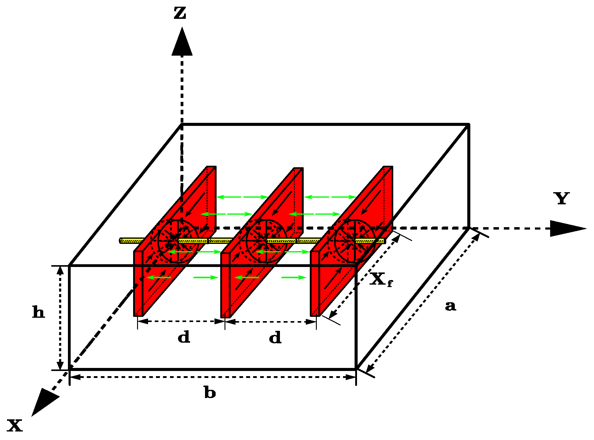
An anisotropic box-shaped reservoir with closed boundaries on all six sides is assumed. The permeabilities in the x, y and z directions are denoted by k_x, k_y and k_z, respectively. Porosity ($\phi$) is constant. The reservoir fluid is a single-phase slightly compressible fluid with total compressibility $C_t$. At the initial time, the pressure is uniform throughout the reservoir and equals the initial reservoir pressure $P_{\mathrm{ini}}$. For the purpose of complex-structured well development and completion design, the wellbore is divided axially into n completion stages, each of which is treated as an equivalent connectivity unit between the well and the reservoir and is distributed along the wellbore at a prescribed spacing. To enhance well–reservoir connectivity, hydraulic fracturing is performed during completion, so that fluids enter the wellbore mainly through local high-conductivity regions. The fracture generated by stimulation is located at the center of each completion stage, with fracture half-length $x_f$ and fracture width $y_d$, as shown in Figure 1. The red squares in the figure represent the schematic geometry of hydraulic fractures located at the center of each completion interval.

By modeling each completion interval as a line-source or plane-source element located within the reservoir at spatial position (x₀, y₀, z₀), the pressure drop induced by a unit-strength source at any arbitrary point (x, y, z) in space can be expressed as [22]:

$$\Delta p_i(t)={\displaystyle \frac{1}{\varphi C_t}}{\displaystyle {\int }_0^t{S}_1{S}_2{S}_{3}d\tau (0<i\le n)}$$

(1)

$$S_1(x,x_0,\tau )={\displaystyle \frac{x_f}{a}}[1+{\displaystyle \frac{4a}{\pi x_f}}{\displaystyle \sum _{n=1}^{\infty }\frac{1}{n}\exp (-\frac{n^2{\pi }^2{k}_x\tau }{\alpha a^2}})\sin {\displaystyle \frac{n\pi x_f}{2a}}\cos {\displaystyle \frac{n\pi x_0}{a}}\cos {\displaystyle \frac{n\pi x}{a}}]$$

(2)

$$S_2(y,y_0,\tau )={\displaystyle \frac{y_d}{b}}[1+{\displaystyle \frac{4b}{\pi y_d}}{\displaystyle \sum _{n=1}^{\infty }\frac{1}{n}\exp (-\frac{n^2{\pi }^2{k}_y\tau }{\alpha b^2}})\sin {\displaystyle \frac{n\pi y_d}{2b}}\cos {\displaystyle \frac{n\pi y_0}{b}}\cos {\displaystyle \frac{n\pi y}{b}}]$$

(3)

$$S_3(z,z_0,\tau )=1+{\displaystyle \frac{4}{\pi }}{\displaystyle \sum _{n=1}^{\infty }\frac{1}{n}\exp (-\frac{n^2{\pi }^2{k}_z\tau }{\alpha h^2}})\sin {\displaystyle \frac{n\pi }{2}}\cos {\displaystyle \frac{n\pi z_0}{h}}\cos {\displaystyle \frac{n\pi z}{h}}$$

(4)

where $\alpha =\phi \mu C_t$, and μ is the reservoir fluid viscosity (mPa·s); S₁, S₂, and S₃ represent the instantaneous Green’s functions in the x, y, and z directions, respectively; and a, b, and h denote the reservoir length, width, and thickness (m). For cases where the fracture is neither parallel nor perpendicular to the boundaries, the coordinates can be rotated and translated before being substituted into the above equation.

2.2. Flow Model for Fractures and the Wellbore

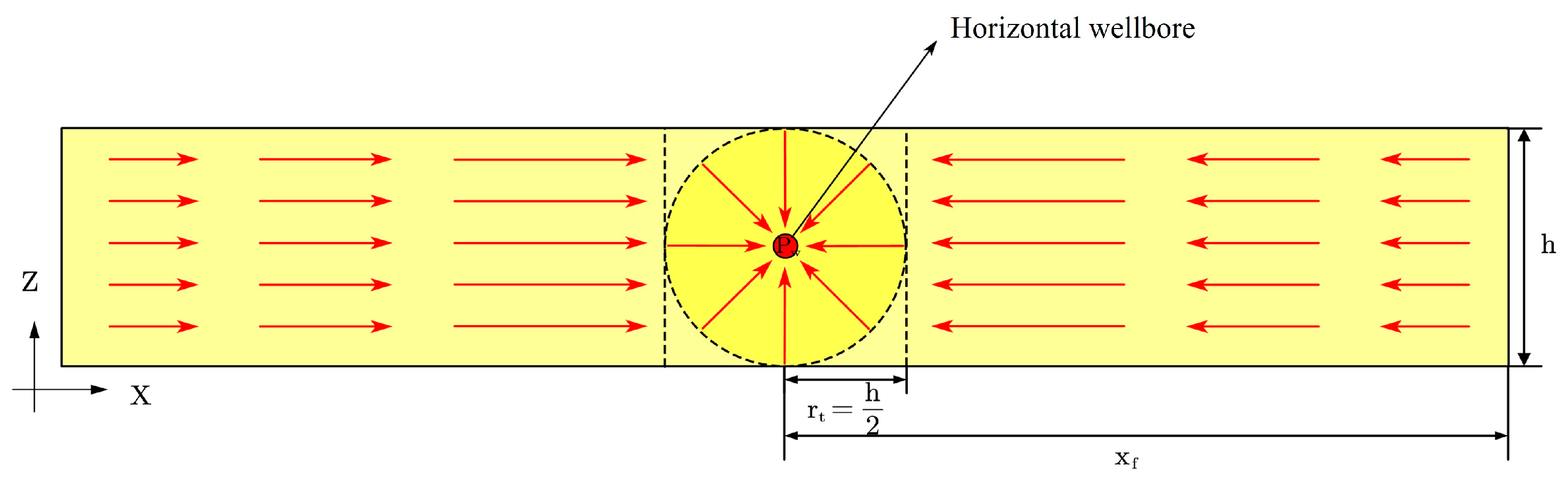
To construct the coupled reservoir–fracture–wellbore flow model, the wellbore is discretized into individual completion stages. Within a single stage, the hydraulic fracture is divided along its control volume into a far-field region and a near-wellbore region. The far-field region is dominated by linear flow, whereas the near-wellbore region is dominated by radial flow, as illustrated in Figure 2.

Physically, this treatment separates the dominant flow regimes inside the fracture, so that the far-field contribution from the reservoir side and the near-wellbore inflow behavior can be represented in a simplified but coupled manner.

The pressure drop within a fracture can be calculated as:

$$\Delta p_{f,i}=p_{e,i}-p_{w,i}=q_i\bullet p_{rf,i}={\displaystyle \frac{q_i\mu }{2\pi k_{f,i}{y}_{d,i}}}[\ln ({\displaystyle \frac{h}{2r_w}})+{\displaystyle \frac{\pi x_{f,i}}{h}}-1+S]$$

(5)

where p_e,i is the reservoir pressure at the tip of fracture i (MPa); p_w,i is the wellbore pressure at the intersection between fracture i and the completion stage (MPa); p_rf,i is the pressure drop per unit rate within fracture i (MPa); q_i is the flow rate of fracture i (m³/s); x_f,i denotes the fracture length of fracture i; y_d,i denotes the fracture width of fracture i; k_f,i, y_d,i denotes the fracture conductivity of fracture i; r_w is the wellbore radius (m); and S is the skin factor.

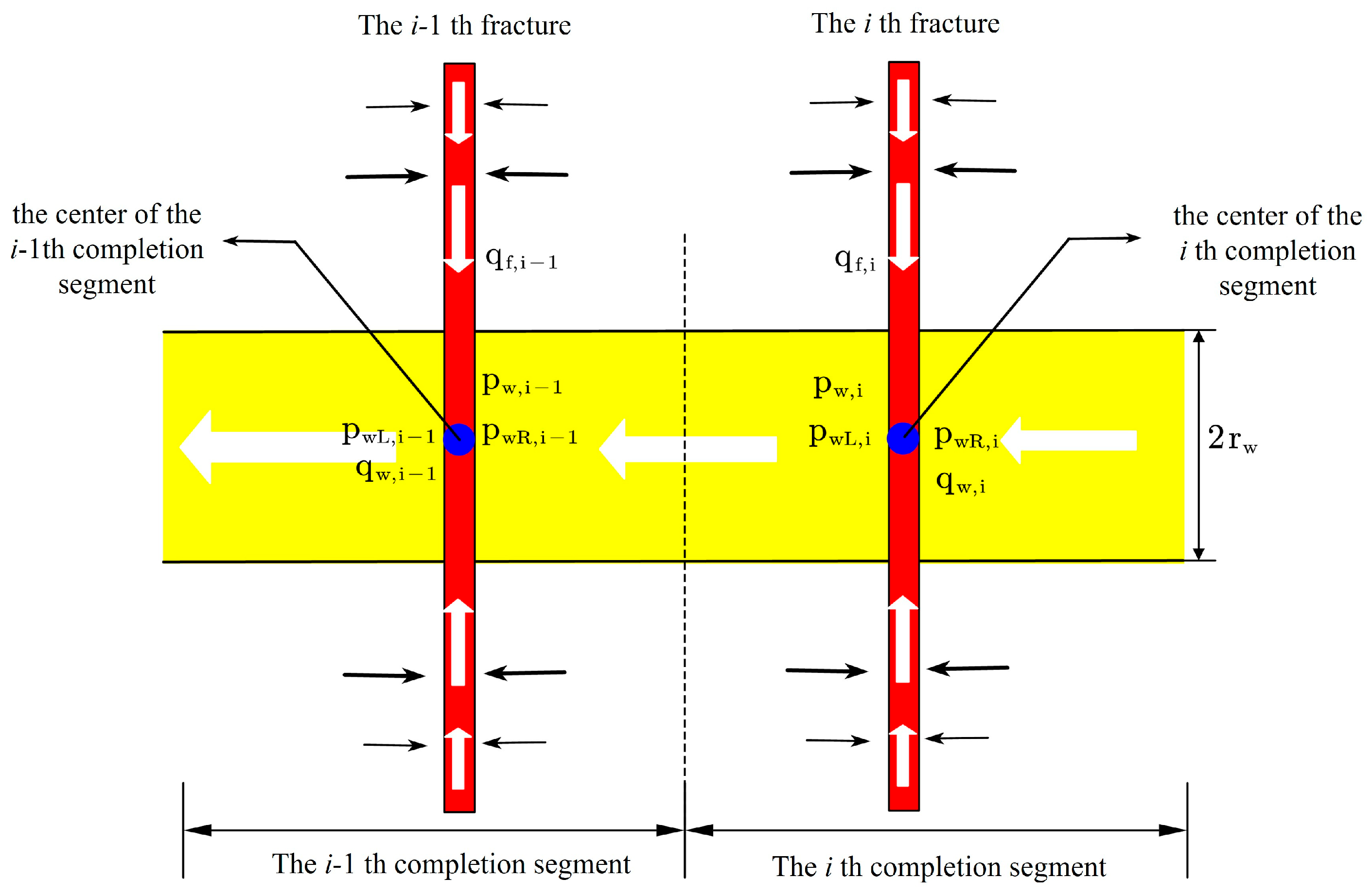
Consider completion stage i and stage i − 1 along the wellbore, whose lengths are li and li − 1, respectively (Figure 3). The fluid is assumed to be single-phase incompressible Newtonian fluid, without heat exchange with the surroundings, and the segment is horizontal with no elevation difference. This assumption is adopted only for the local pressure-drop calculation of the wellbore segment, whereas the reservoir flow in Section 2.1 is still described by the single-phase slightly compressible formulation.

The pressure drop between adjacent completion stages is given by:

$$\Delta p_w=\Delta p_d+\Delta p_a+\Delta p_g$$

(6)

$$\Delta p_{d,i}={\displaystyle \frac{{\tau }_w{l}_i}{r_w}}={\displaystyle \frac{C_f{f}_i\rho q_{w,i}^2{l}_i}{r_w^5}}$$

(7)

Equation (7) is obtained by applying the momentum balance to the wellbore segment between two adjacent stages and expressing the wall shear stress through the friction-factor relation. After substituting the shear-stress term into the segment momentum equation, the general form of the frictional pressure drop is obtained.

$$\Delta p_{a,i}={\displaystyle \frac{C_f\rho q_{w,i}{q}_{f,i}}{r_w^4}}$$

(8)

$$\Delta p_g=p_{w,i-1}-p_{w,i}=\rho g{l}_i\cos \theta$$

(9)

where Δp_d, Δp_a, and Δp_g are the frictional, acceleration, and gravitational pressure drops in the wellbore, respectively; τ_w is the shear stress at the wellbore wall; C_f is a unit conversion factor; f_i is the friction factor between stages i and i − 1. Here, f_i denotes the local wellbore friction factor for the segment between stages i and i − 1, evaluated according to the local flow regime determined by the segment flow velocity. In this study, f_i denotes the Darcy friction factor and is evaluated according to the local flow regime in the corresponding segment. For laminar flow, f_i = 64/Re_i; for turbulent flow, the Blasius correlation is used. Here, Rei is the Reynolds number of segment i. l_i is the distance between stages i and i − 1; and θ is the well deviation angle.

2.3. Coupled Reservoir-Fracture-Wellbore Model

In this work, a nodal analysis approach is used to construct the coupled reservoir–fracture–wellbore model. Wellbore nodes are defined at the fracture–wellbore interfaces, located at the center of each completion stage, and reservoir nodes are located at the center of each fracture. According to the flow process, a total of 6n unknowns are introduced: (1) reservoir–node pressures p_e,1, p_e,2, …, p_e,n; (2) node pressures at the center of each completion stage p_w,1, p_w,2, …, p_w,n; (3) pressures on the left side of each stage node p_wL,1, p_wL,2, …, p_wL,n; (4) pressures on the right side of each stage node p_wR,1, p_wR,2, …, p_wR,n; (5) flow rates from the reservoir nodes into fractures q_f,1, q_f,2, …, q_f,n; and (6) flow rates in the wellbore at stage-node q_w,1, q_w,2, …, q_w,n.

From a physical viewpoint, the coupled model is used to determine how pressure and flow are distributed among the reservoir, fractures, and wellbore segments, so that the inflow contribution of each completion stage can be solved simultaneously.

Assuming a constant fluid density for the reservoir, fractures, and wellbore, the mass conservation equations for the n stage nodes can be expressed as:

$$q_{w,i}={\displaystyle \sum _{j=i}^n{q}_{f,j}}\begin{array}{cc}& \end{array}(i=1,2,\dots ,n)$$

(10)

Because the stage-node pressure can be taken as the average of the pressures on its two sides, n equations relating the stage-node pressure to the left and right pressures can be written as:

$$p_{w,i}={\displaystyle \frac{p_{wL,i}+p_{wR,i}}{2}}\begin{array}{cc}& \end{array}(i=1,2,\dots ,n)$$

(11)

where, p_w,i is the average stage-node pressure, while p_wL,i and p_wR,i are the pressures on the left and right sides of the same node, respectively.

Since q_w,i can be substituted by q_f,i and p_w,i can be expressed in terms of p_wL,i and p_wR,i, the 6n unknowns can be reduced to 4n unknowns. To solve these 4n unknowns, 4n independent equations are required.

(1) Reservoir flow equations (n equations):

Let the coordinates of the reservoir node associated with fracture i be (x_0,i, y_0,i, z_0,i). The pressure drop at this point is the superposition of the pressure drops induced by all reservoir nodes, which can be expressed as:

$$\Delta P_i(t)=p_{ini}-{\displaystyle {\displaystyle \sum _{j=1}^n}p((x_{0,i},y_{0,i},z_{0,i});(x_{0,j},y_{0,j},z_{0,j});t)}={\displaystyle {\displaystyle \sum _{j=1}^n}{q}_j}\Delta p_{ij}(t)$$

(12)

where q_j represents the flow rate of the j-th fracture; p((x_0,i, y_0,i, z_0,i); (x_0,j, y_0,j, z_0,j); t) denotes the pressure drop induced by the j-th fracture at the reservoir node (x_0,i, y_0,i, z_0,i) of the i-th fracture at time t; and Δp_ij(t)is the pressure drop caused by a source of unit strength of the j-th fracture at the reservoir node (x_0,i, y_0,i, z_0,i) of the i-th fracture. For variable flow rates, applying Duhamel’s principle yields the pressure drop at any point in the formation as:

$$\Delta p_i={\displaystyle {\int }_0^t{\displaystyle \sum _{j=1}^n{q}_j(\tau )\left[-\frac{d{p}_{ij}(t-\tau )}{d\tau }\right]}}d\tau (i=1,2,\dots n)$$

(13)

By selecting an appropriate time step (Δt) and discretizing at the k-th time level, combining Equations (12) and (13) yields a numerical integration form with respect to time step:

$$\begin{array}{r}{\displaystyle {\displaystyle \sum _{j=1}^n}{q}_j^k}{p}_{ij}(\Delta t)+p_i(t^k)=p_{ini}-{\displaystyle {\displaystyle \sum _{m=1}^{k-1}}{\displaystyle \sum _{j=1}^n{q}_j}}(t^m)[p_{ij}((k-m+1)\Delta t)-p_{ij}((k-m)\Delta t)]\\ (i=1,2,\dots ,n;k=1,2,3,\dots ,)\end{array}$$

(14)

where

$$p_{ij}(0)=0p_{ij}(t^k-t^{k-1})=p_{ij}(\Delta t)\Delta P_i=p_{ini}-p_i(t^k)t^k=k\times \Delta t.$$

(2) Fracture flow equations (n equations):

Taking the fracture in completion stage i as an example, the pressure drop between the reservoir–node pressure p_e,i and the pressures on the left and right sides of the wellbore node, p_wL,i and p_wR,i, can be written as:

$$p_{e,i}-({\displaystyle \frac{p_{wL,i}+p_{wR,i}}{2}})=q_{f,i}\bullet p_{rf,i}={\displaystyle \frac{q_{f,i}\mu }{2\pi k_{f,i}{y}_{d,i}}}[\ln ({\displaystyle \frac{h}{2r_w}})+{\displaystyle \frac{\pi x_{f,i}}{2h}}-1+S]$$

(15)

(3) Wellbore flow Equations (2n − 1 equations):

Consider completion stage i. The fluid within this stage consists of the inflow from fracture i and the fluid from stage i + 1. When the fluid flows from the right side of the stage-i node to the left side, the acceleration pressure drop between p_wL,i and p_wR,i can be expressed as:

$$p_{wR,i}-p_{wL,i}=\Delta p_{a,i}={\displaystyle \frac{C_f\rho q_{w,i-1}{q}_{f,i}}{r_w^4}}$$

(16)

where q_w,i−1 denotes the wellbore flow rate approaching stage i, and q_f,i denotes the inflow from fracture i. Their simultaneous appearance reflects the mixing process at the stage node, where the newly entering fracture flow changes the total wellbore flow rate and causes a momentum variation, thereby giving rise to the acceleration pressure drop.

When the fluid flows from completion stage i to completion stage i − 1, the frictional pressure drop between p_wL,i and p_wR,i−1 can be expressed as:

$$p_{wL,i}-p_{wR,i-1}=\Delta p_{d,i}={\displaystyle \frac{C_f{f}_i\rho q_{w,i}^2{l}_i}{r_w^5}}$$

(17)

By substituting q_w,i with q_f,i, a set of 2n − 1 nonlinear wellbore pressure-drop equations in terms of q_f,1, q_f,2, …, q_f,n, p_wL,1, p_wL,2, …, p_wL,n, and p_wR,1, p_wR,2, …, p_wR,n can be obtained.

If an elevation difference exists between two completion-interval nodes, the pressure drop between the pressure on the left side of the i-th node, p_wL,i, and the pressure on the right side of the (i − 1)-th node, p_wR,i−1, is defined as the sum of the frictional pressure drop, Δp_d,i, and the gravitational pressure drop, Δp_g,i. For the reported cases, the completion-stage segments are horizontal, so the gravitational contribution is negligible. This relationship is denoted as:

$$p_{wL,i}-p_{wR,i-1}=\Delta p_{d,i}+\Delta p_{g.i}={\displaystyle \frac{C_f{f}_i\rho q_{w,i}^2{l}_i}{r_w^5}}+\rho g{l}_i\cos \theta$$

(18)

(4) Constraint equation:

Rate constraint: for constant-rate production, the total well production rate remains constant at any time, which can be expressed as:

$$q_{w,1}={\displaystyle \sum _{j=1}^n{q}_{f,j}}=Q$$

(19)

Bottomhole pressure constraint: for constant-bottomhole flowing pressure (BHP) production, the pressure at the first wellbore node satisfies:

$$p_{wf}-\left({\displaystyle \frac{p_{wL,1}+p_{wR,1}}{2}}\right)=\Delta p_{d,1}={\displaystyle \frac{C_f{f}_1\rho q_{w,1}^2{l}_1}{r_w^5}}$$

(20)

In this case, the number of equations equals the number of unknowns, and the system can be solved using the Newton–Raphson iteration method. In the numerical implementation, the reservoir flow term is discretized in time using the selected time step Δt, and the coupled nonlinear system is solved iteratively by the Newton–Raphson method until convergence is reached. In the present implementation, convergence is declared when the relative change in the unknown variables between two successive iterations is smaller than a prescribed tolerance. A sufficiently small time step is selected to maintain numerical stability of the transient calculation. In each iteration, the Jacobian matrix is assembled from the coupled pressure-rate equations and updated until the convergence criterion is satisfied.

2.4. Establishment of the Productivity Model for Complex-Structured Fractured Wells

Complex-structured wells can be designed with different well trajectories according to reservoir types and geological conditions to achieve efficient development. Common complex well types in engineering practice include long horizontal wells, multilateral wells, and multi-toe wells. These configurations can be used for single-layer development as well as for commingled production from multiple layers. This study focuses on complex-structured horizontal wells and complex-structured multilateral wells. Although the validation examples in this work focus on a fractured horizontal well and a fishbone-shaped multilateral well, the underlying coupled reservoir–fracture–wellbore formulation is not restricted to fishbone geometry. From a modeling standpoint, a multi-toe well can also be represented as a main wellbore/branch wellbore network with a different branch distribution and node connectivity, and the same coupling framework can be applied after updating the geometric description and control-unit arrangement.

In Section 2.3, a productivity model was established for a single wellbore under staged-completion conditions, taking into account wellbore–reservoir coupling. For complex-structured wells, the governing mechanisms of reservoir flow and pipe flow are consistent with those of a single well model; the key difference lies in the more complex wellbore architecture, involving multiple branch wellbores and the commingling process between branches and the main wellbore. Therefore, based on the model in Section 2.3, a unified description of complex-structured well productivity can be achieved by appropriately simplifying and extending the wellbore structure.

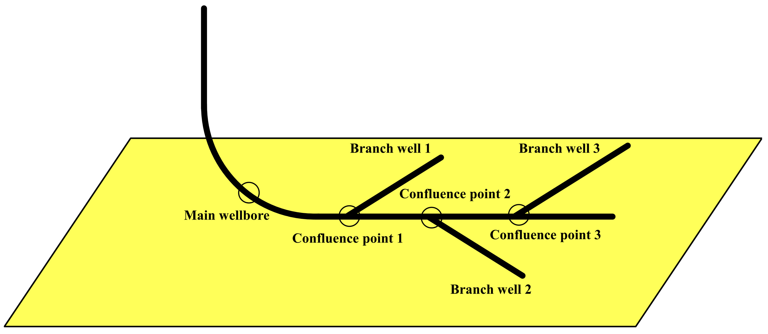
For the complex-structured wells considered here, completion stages and hydraulic fractures are distributed only in the branch wellbores. Fluids from each branch flow into the main wellbore and then are produced to the wellhead through the main wellbore. Based on this architecture, the complex-structured well can be simplified as a wellbore network system consisting of a main wellbore and multiple branches, as shown in Figure 4.

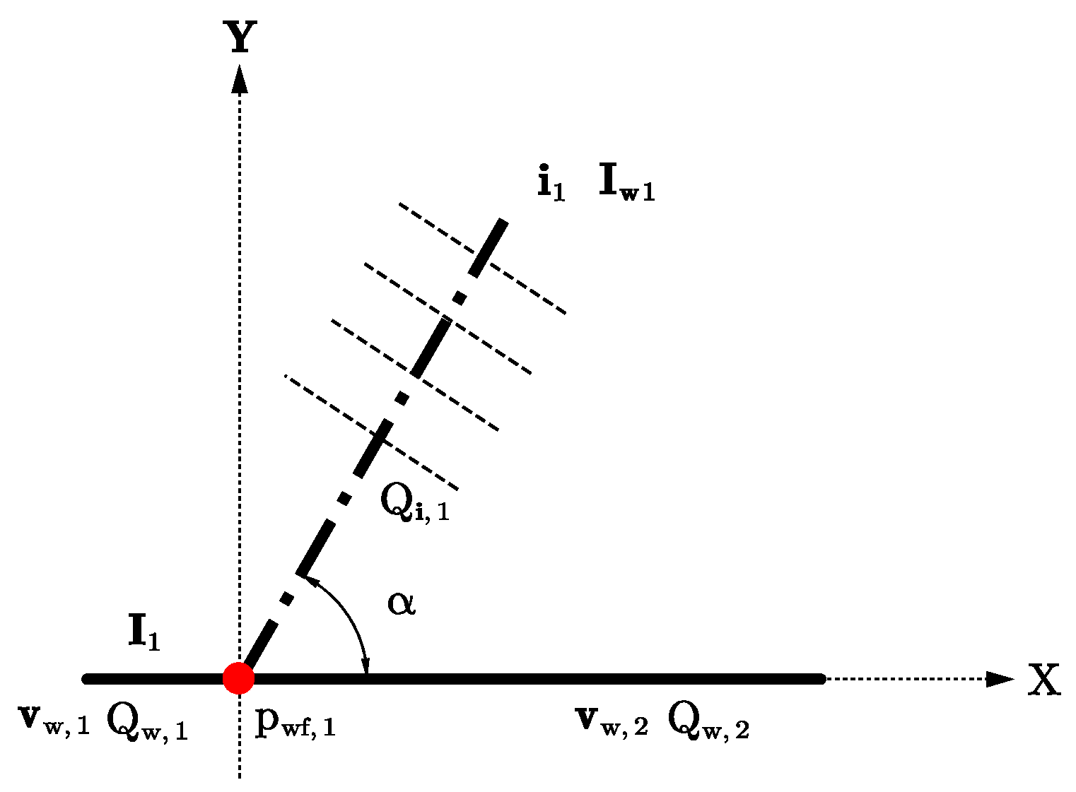
The coupled seepage and pipe-flow process within each branch can be described directly by the staged-completion wellbore model developed in Section 2.3. In contrast, the flow behavior at the junction between a branch and the main wellbore requires consideration of the local pressure loss caused by the confluence of multiple streams. To this end, based on momentum and energy conservation, a model is developed for the pressure change at the junction between a branch and the main wellbore. For convenience, the confluence segment of a branch and the main wellbore is simplified as shown in Figure 5.

When the fluid from a branch wellbore enters the main wellbore, a local pressure loss occurs at the junction. This loss depends on the branch flow rate, the angle between the branch and the main wellbore, and wellbore geometry. As this study focuses on the confluence process, the effects of the frictional pressure drop along the wellbore and the gravitational pressure drop due to an elevation difference are neglected. The flow velocity in the main wellbore can be determined from the flow rate in the corresponding direction as:

$$V_{w,1}={\displaystyle \frac{Q_{w,1}}{A}}\begin{array}{cc}& \end{array}{V}_{w,2}={\displaystyle \frac{Q_{w,2}}{A}}$$

(21)

where A is the cross-sectional area of the main wellbore (m²); i denotes the main wellbore direction (i = 1, 2); and Q_w,i is the flow rate in direction i (m³/d).

Assume that the branch contains i₁ completion stages, with branch production rate Q_i,1 and the pressure at the branch root p_i,1. At the intersection with the main wellbore, the pressure is p_wf,1; the pressure and flow rate at the left end of the main wellbore segment are p_wfL,1 and Q_w,1, respectively, and those at the right end are p_wfR,1 and Q_w,2, respectively. According to Figure 5, the momentum equation, energy equation, and continuity equation of the fluid at the junction in the main wellbore direction can be written as follows:

$$p_{wfR,1}\cdot A-p_{wfL,1}\cdot A+F_x=\rho Q_{w,1}{v}_{w,1}-\rho Q_{w,2}{v}_{w,2}$$

(22)

$${\displaystyle \frac{p_{wfR,1}}{\rho g}}+{\displaystyle \frac{v_{w,2}^2}{2g}}={\displaystyle \frac{p_{wfL,1}}{\rho g}}+{\displaystyle \frac{v_{w,1}^2}{2g}}+h_{12}$$

(23)

$$v_{w,2}\cdot A+Q_{i,1}=v_{w,1}\cdot A$$

(24)

where h₁₂ represents the energy loss between the two segments, and A represents the cross-sectional area of the main wellbore, m².

In Equation (22), F_x represents the force exerted by the pipe wall on the fluid at the junction, which is given by:

$$F_x=\rho {\displaystyle \frac{Q_{i,1}^2}{A_i}}\cos \alpha$$

(25)

According to Equations (22) and (25), the following expression can be obtained:

$$p_{wfR,1}-p_{wfR,2}={\displaystyle \frac{\rho }{A}}(Q_{w,1}{v}_{w,1}-Q_{w,2}{v}_{w,2}-{\displaystyle \frac{Q_{i,1}^2}{A_i}}\cos \alpha )$$

(26)

According to Equation (23), the expression for the energy loss term h₁₂ can be obtained as:

$$h_{12}={\displaystyle \frac{1}{\rho g}}(p_{wfR,1-}{p}_{wfL,1})+{\displaystyle \frac{1}{2g}}(v_{w,2}^2-v_{w,1}^2)$$

(27)

By combining Equations (24), (26) and (27), the following expression is obtained:

$$h_{12}={\displaystyle \frac{Q_{i,1}^2+2v_{w,2}{Q}_{i,1}A}{2g{A}^2}}-{\displaystyle \frac{Q_{i,1}^2\cos \alpha }{A{A}_i}}$$

(28)

Thus, the pressure drop at the branch junction, Δp_a, is:

$$\Delta p_a=p_{wfR,1}-p_{wfL,1}=h_{12}\rho g+{\displaystyle \frac{\rho Q_{i,1}^2}{2A^2}}+{\displaystyle \frac{v_{w,2}{Q}_{i,1}\rho }{A}}$$

(29)

After calculating the internal flow within each branch and the pressure loss at the junctions, the branches and the main wellbore can be treated as a wellbore network composed of multiple discretized control units. Combined with the reservoir–fracture–wellbore coupling model described above, an iterative solution can be used to jointly solve the flow allocation among completion stages and the bottomhole flowing pressure, thereby obtaining the overall productivity of complex-structured fractured wells. The reservoir, fracture, and wellbore sub-models are discretized and coupled through nodal continuity, and the resulting nonlinear system is solved iteratively; during optimization, this semi-analytical model is repeatedly called by the genetic algorithm for different parameter combinations.

3. Model Validation

To verify the accuracy and applicability of the proposed coupled reservoir–fracture–wellbore semi-analytical productivity model, both water–electric analogy physical experiments and field production data are used for validation. The water–electric analogy experiments are employed to test the model’s predictive capability under different fracture-parameter settings, while the field case is used to examine engineering applicability under actual reservoir conditions.

3.1. Validation Using Water-Electric Analogy Experiments

The water–electric analogy experiment is a commonly used physical simulation method for reservoir flow. Based on the water–electric similarity principle, the reservoir seepage process is represented by an electric current field; the measured current is used to equivalently characterize well production. When similarity criteria are satisfied, the geometric configuration, boundary conditions, and physical properties of the experimental setup can be scaled to the actual reservoir, enabling physical simulation of reservoir flow behavior. This analogy is adopted here based on the formal similarity between the seepage field and the electric-current field under the assumed conditions.

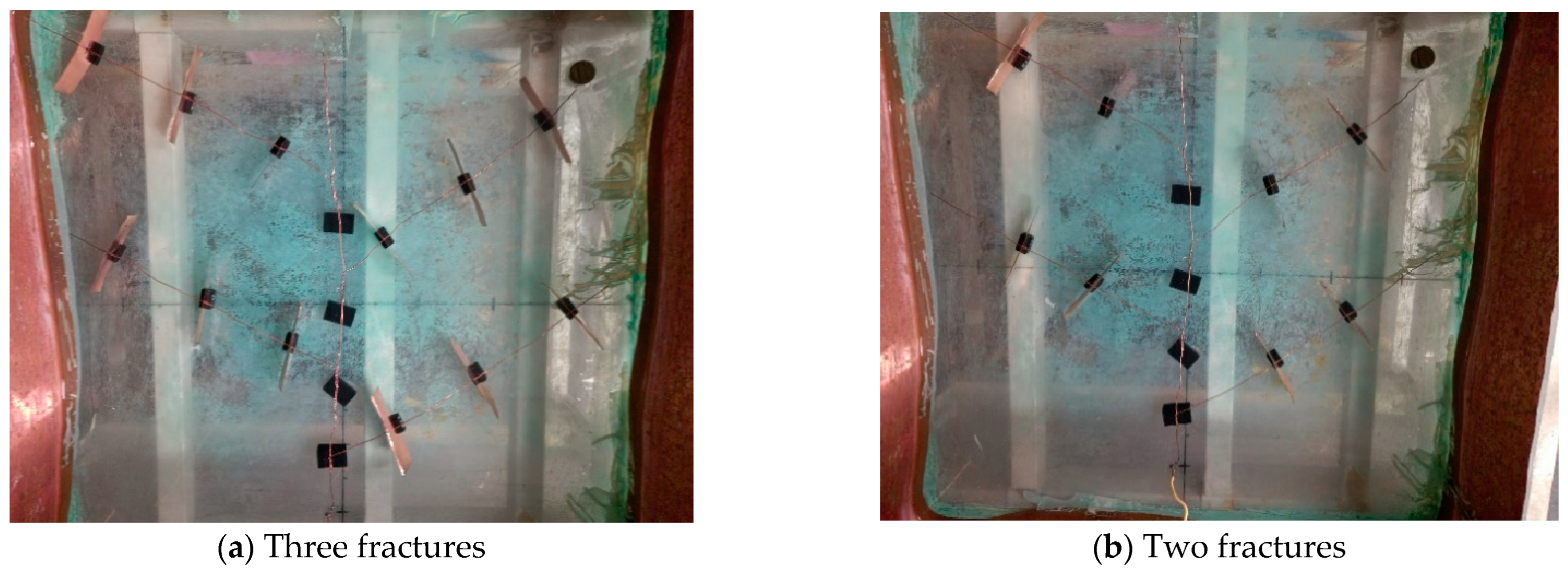
To validate the coupled reservoir–fracture–wellbore semi-analytical model, a fishbone-shaped multilateral complex-structured well experimental setup was built based on the water–electric analogy principle for different numbers of fractures. By varying the number of fractures, fracture half-length, and fracture spacing, the corresponding current values were measured and converted into theoretical experimental production, which was then compared with model predictions. The experimental setup consists of a reservoir simulation system, a low-voltage circuit system, measuring points, and a data acquisition system. The similarity between the electrical model and the reservoir flow system is established through corresponding geometric, pressure, and flow rate scaling relations. The experimental setup is shown in Figure 6. Different fracture configurations were generated by varying fracture number, fracture half-length, and fracture spacing under the same similarity framework.

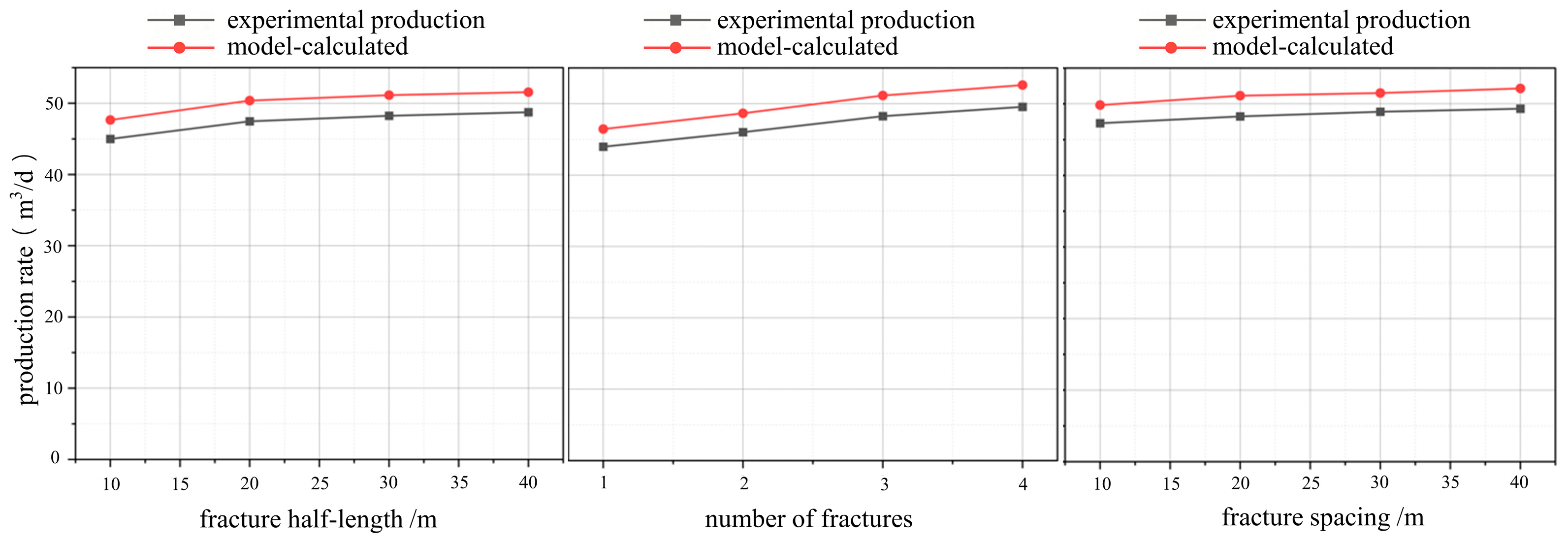
The theoretical experimental production q′ was compared with the model-predicted production q, and the relative deviation was calculated to evaluate model accuracy. The measured current I, the theoretical experimental production q′, the model production q, and the relative deviation are summarized in

Table 1. Comparison between theoretical production from water–electric analogy experiments and semi-analytical model predictions for a fishbone-shaped complex-structured multilateral well.

Fracture Configuration (Experimental Model)	Current (mA)	Theoretical Production (m3/d)	Model Prediction (m3/d)	Relative Error (%)
3 fractures, length 4 cm, spacing 8 cm	25.197	44.993	47.658	5.92
3 fractures, length 8 cm, spacing 8 cm	26.585	47.473	50.383	6.13
3 fractures, length 12 cm, spacing 8 cm	27.015	48.241	51.145	6.02
3 fractures, length 16 cm, spacing 8 cm	27.293	48.738	51.555	5.78
1 fractures, length 12 cm, spacing 8 cm	24.620	43.965	46.436	5.62
2 fractures, length 12 cm, spacing 8 cm	25.766	46.011	48.657	5.75
4 fractures, length 12 cm, spacing 8 cm	27.749	49.552	52.610	6.17
3 fractures, length 12 cm, spacing 4 cm	26.487	47.298	49.829	5.35
3 fractures, length 12 cm, spacing 12 cm	27.380	48.893	51.519	5.37
3 fractures, length 12 cm, spacing 16 cm	27.615	49.313	52.153	5.76

. Theoretical experimental production q′ and model-predicted production q under different fracture configurations are plotted in Figure 7.

The measured current I (mA) is converted into the theoretical production rate q′ (m³/d) using the established similarity relation for the water–electric analogy experiment.

As shown in Figure 7 and Table 1, the relative error between the semi-analytical model predictions and the theoretical experimental production is within 7%, indicating good predictive accuracy of the proposed model. The relative error between model predictions and experimental measurements is within approximately 7% for all tested fracture-parameter combinations, and further increases in fracture conductivity yield diminishing marginal gains in production, consistent with the trend observed in Table 1. It is also observed that, under the experimental conditions considered, the incremental production gain diminishes as the number of fractures, fracture half-length, and fracture spacing increase. This suggests that the reservoir has been stimulated relatively effectively in the fishbone fractured-well configuration, and further enlarging the stimulation scale yields limited marginal benefit in production. These results underline the necessity of optimizing completion and fracturing parameters.

3.2. Validation Using a Field Case

To further validate the model under actual reservoir conditions, a hydraulically fractured horizontal well A20 in the BZ oilfield, a typical low-permeability reservoir in the Bohai Sea, was selected as a case study. The semi-analytical model predictions were compared with field production data. The basic reservoir parameters and the geometric parameters of the wellbore and fractures are listed in

Table 2. Basic reservoir parameters.

Parameter	Value	Unit
Reservoir depth	3281	m
Reservoir length	3000	m
Reservoir width	3000	m
Reservoir thickness	13.3	m
Permeability	30	mD
Reservoir pressure	35	MPa
Initial drawdown	14	MPa
Porosity	10	%
Formation volume factor	1.3	m3/m3
Oil viscosity	1.25	mPa·s
Skin factor	8.7	/
Total compressibility	1.5 × 10−3	MPa−1
Oil density	0.96	g/cm3

and

Table 3. Basic wellbore and fracture parameters for the field validation case.

Parameter	Value	Unit
Wellbore length	1500	m
Wellbore radius	0.054	m
Wellbore position in x-direction (x0)	1500	m
Wellbore toe location in y-direction (y1)	750	m
Wellbore heel location in y-direction (y2)	2250	m
Wellbore position in z-direction (z0)	6.651	m
Number of completion stages	4	/
Stage spacing	300	m
Fracture half-length	95	m
Fracture width	0.01	m
Fracture conductivity	125	D·cm

, respectively.

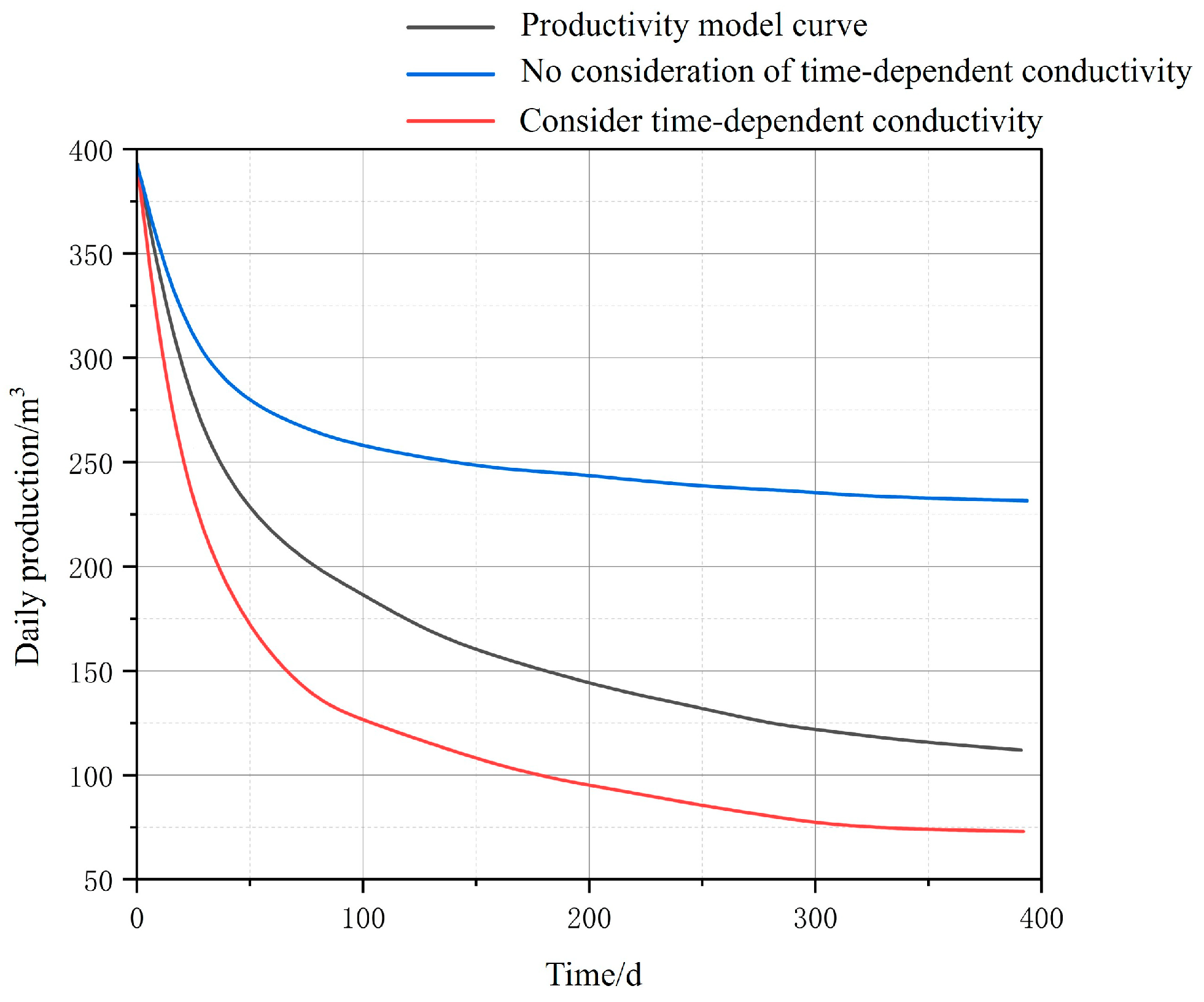
Using the above parameters, a semi-analytical productivity model was constructed, and the daily production rate over 400 days was compared with field data, as shown in Figure 8.

As shown in Figure 8, the predicted daily production trend from the semi-analytical model is generally consistent with the field data, and the model captures the production decline behavior during the production period. It should be noted that, compared with some models in the literature, the present model accounts for both in-fracture flow and wellbore pressure drop, but does not further incorporate time-dependent changes in fracture conductivity. As a result, the model predictions fall between the prediction curves of different models over certain time ranges while remaining within a reasonable band.

Overall, the validations based on water–electric analogy experiments and the field case demonstrate that the proposed coupled reservoir–fracture–wellbore semi-analytical model provides satisfactory prediction accuracy under different fracture parameter conditions, and can serve as a reliable basis for subsequent optimization of completion and fracture parameters in complex-structured wells. In addition, the productivity model was checked against KAPPA numerical simulation results for a multilateral fractured-well case, with the relative deviation remaining within 8%. This comparison further supports the credibility of the productivity model, although it is not intended as a direct validation of the GA optimization result itself.

4. Genetic-Algorithm-Based Optimization of Completion and Fracture Parameters

During the development of complex-structured wells, the completion staging scheme and fracture parameters jointly determine the distribution of inflow capacity along the wellbore. Their combined effects are highly nonlinear and often multi-modal, making it difficult for traditional analytical optimization methods to obtain a global optimum. Genetic algorithms (GA), which are global optimization methods based on natural selection and genetic mechanisms, require little continuity of the objective function and offer strong global search capability; they have been widely applied to complex oil and gas engineering optimization problems. Based on GA theory and the semi-analytical productivity model developed in this study, a joint optimization framework is established for completion staging parameters and fracture-geometry parameters. The optimization requires specification of the objective function, constraints, ranges of decision variables, and an encoding strategy. In the optimization process, each candidate parameter set generated by the GA is evaluated through the semi-analytical productivity model to calculate production performance and the corresponding NPV.

4.1. Objective Function

To fully account for economic performance and investment return, net present value (NPV) over a given period is selected as the objective function for optimizing completion staging parameters and fracture-geometry parameters. This objective reflects the direct impact of cumulative oil production and also incorporates fixed capital expenditure as well as costs associated with fracturing and drilling, providing an economic perspective for the evaluation and optimization of completion design for complex-structured wells. The objective function is formulated as:

$$NPV={\displaystyle \sum _{t=1}^T}{\displaystyle \frac{q_{o,t}\mathsf{\Delta }t{V}_F}{{(1+r)}^t}}-(FC+({\displaystyle \sum _{k=1}^N{C}_{\mathrm{well}}+{\displaystyle \sum _{j=1}^n{C}_{\mathrm{fracture}}}))}$$

(30)

where:

q_o,t—oil production rate at time step t (m³/d);

V_F—oil price (USD/m³);

Δt—length of one production time step (d);

r—discount rate per time step; In the present demonstrative case study, the discount rate is treated as a scenario-dependent economic input and should be specified according to project-specific economic evaluation standards in field applications;

T—total number of time steps over the production period;

FC—fixed cost, including construction management, equipment procurement, labor, etc. (USD);

C_well—drilling and completion cost for one complex-structured well (USD);

C_fracture—cost of creating one hydraulic fracture (USD);

N—number of horizontal well sections;

n—number of fractures (stages).

In this study, an annual discount rate r_annualr of 10% was assumed. For the time-step NPV calculation in Equation (30), the corresponding time-step discount rate was calculated as

$$r={(1+r_{\mathrm{annual}})}^{\Delta t/365}-1$$

(31)

Operating costs, taxes, royalties, and abandonment costs are not explicitly considered; therefore, the objective function should be interpreted as a simplified discounted economic indicator for comparative optimization rather than a complete economic model for field investment decisions.

For a complex-structured fractured well with a fixed architecture, the number of horizontal sections N and the drilling and completion cost per well C_well can be treated as constants, where C_well can be calculated from the horizontal length and the unit drilling and completion cost per meter. Therefore, the dominant factors affecting NPV are the cumulative oil production Q, the number of fractures n, and the cost per fracture C_fracture.

Among these, Q is jointly determined by the completion staging scheme and fracture-geometry parameters. The cost per fracture C_fracture is mainly affected by fracture half-length and fracture conductivity. Based on field investigation and engineering experience, the relationships between cost and fracture half-length and fracture conductivity can be expressed as follows [23]:

(1)

Cost as a function of fracture half-length:

$$C_1=2.77l^2-151.38l+44772$$

(32)

(2)

Cost as a function of fracture conductivity:

$$C_2=15.28{\beta }^2-411.11\beta +72913$$

(33)

where:

C₁—cost associated with fracture half-length (USD);

C₂—cost associated with fracture conductivity (USD);

l—fracture half-length (m);

β—fracture conductivity (D·cm).

Accordingly, the final NPV is calculated as:

$$\begin{array}{l}NPV={\displaystyle \sum _{t=1}^T}{\displaystyle \frac{q_{o,t}\mathsf{\Delta }t{V}_F}{{(1+r)}^t}}-(FC+{\displaystyle \sum _{k=1}^N{C}_{well}+{\displaystyle \sum _{j=1}^n(C_1+C_2)}))}\\ ={\displaystyle \sum _{t=1}^T}{\displaystyle \frac{q_{o,t}\mathsf{\Delta }t{V}_F}{{(1+r)}^t}}-(FC+{\displaystyle \sum _{k=1}^N{C}_{well}+{\displaystyle \sum _{j=1}^n(2.77{l_j}^2-151.38l_j+15.28{{\beta }_j}^2-411.11{\beta }_j+117685)})}\end{array}$$

(34)

The constant term appearing in the converted combined fracture cost expression originates from the sum of the constant components in the two empirical cost correlations adopted from Ref. [23] after unit conversion. Therefore, it should be interpreted as the baseline term embedded in the empirical single-fracture cost function, rather than an additional independently assigned fixed project cost.

These empirical correlations are adopted as simplified cost models for the present case study and are intended to reflect the first-order dependence of fracturing cost on fracture half-length and conductivity. Since actual field costs may vary significantly with reservoir location, service pricing, operational conditions, and completion practices, these cost functions are not intended to represent universally applicable offshore cost models. Therefore, when the proposed optimization framework is applied to other reservoirs or field developments, the cost-function parameters should be recalibrated using local field cost data.

In the present study, the NPV calculation is carried out under fixed economic conditions, and factors such as operating-cost variation, discount-rate uncertainty, and other economic risks are not explicitly included. The economic parameters adopted in this study are listed in

Table 4. Economic parameters used in the objective function.

Economic Parameter	Value
Oil price	79.97 USD/bbl
Fixed capital cost	1.53 × 106 USD
Drilling and completion cost per meter	2.22 × 103 USD

.

4.2. Optimization Variables and Encoding

Based on the literature review and feedback from completion and fracturing operations in the project, the decision variables optimized in this study include the number of completion stages, fracture half-length, stage spacing, and fracture conductivity. The optimization problem can be expressed as:

$$X=\left[x_1,x_2,x_3,x_4\right]$$

(35)

where:

x₁—number of completion stages;

x₂—fracture half-length (m);

x₃—stage spacing (m);

x₄—fracture conductivity (D·cm).

In the genetic algorithm, upper and lower bounds must be specified for each variable, which should be set according to the actual reservoir conditions. In particular, the stage spacing must be constrained by the horizontal section length and the number of completion stages, and the specified range should not exceed the maximum horizontal length.

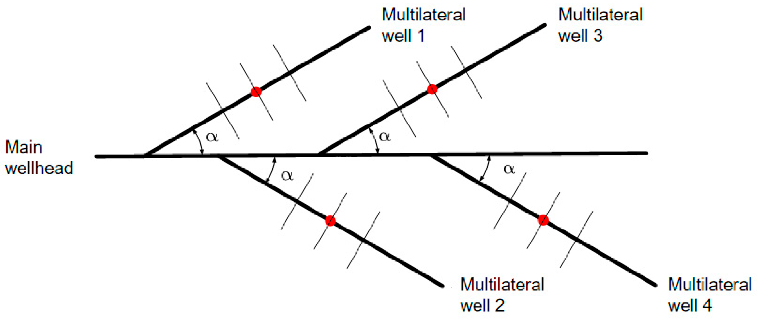
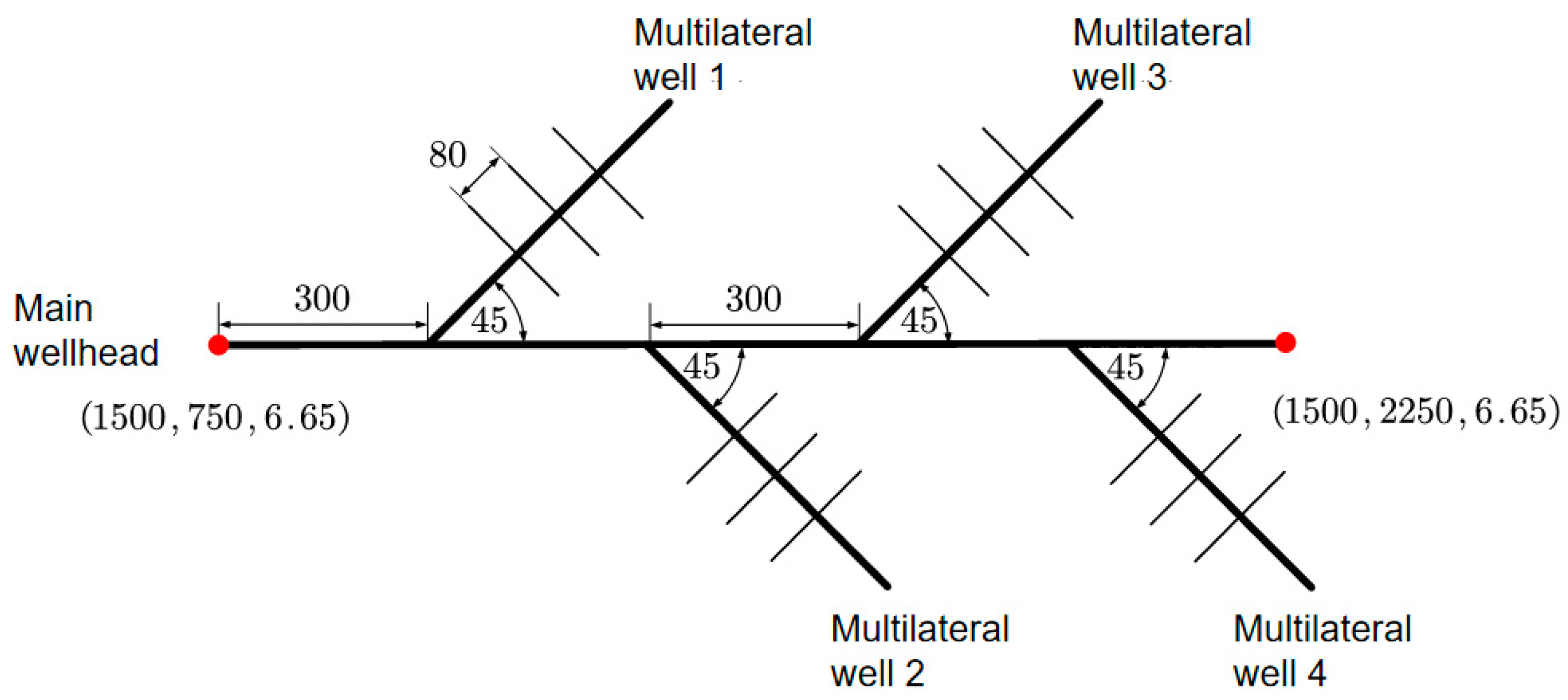
For parameter encoding of a complex-structured well model, the well architecture must first be defined, and the system can be decomposed into multiple multi-stage fractured horizontal laterals connected to a main wellbore. Taking a four-branch fishbone fractured well as an example, the well can be represented as the combination of four multi-stage fractured laterals and a main wellbore, as shown in Figure 9.

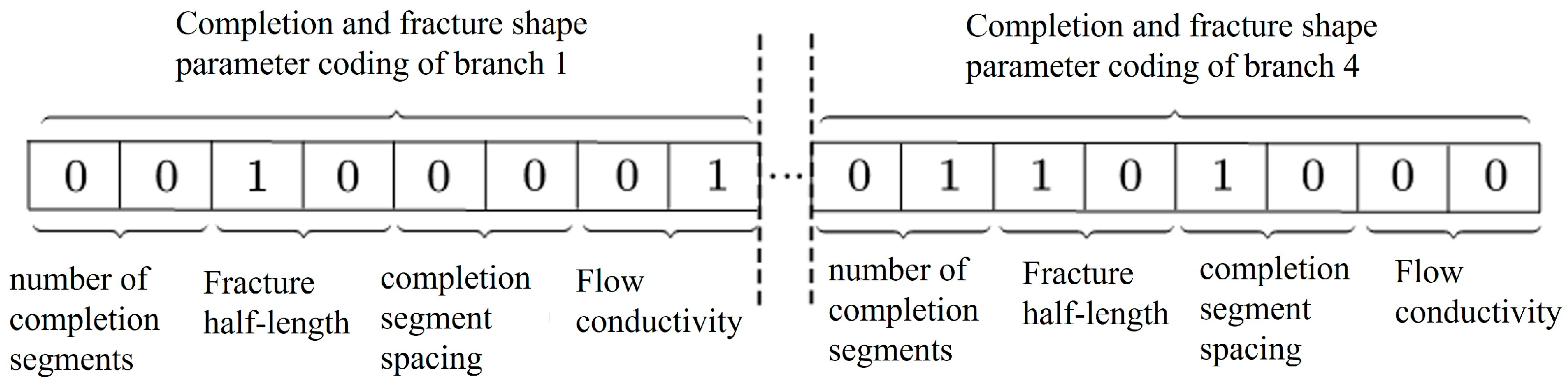
For a single branch, the completion parameters and fracture-geometry parameters are encoded with a binary length determined by the variable ranges and step sizes. The encoding for the entire complex-structured well is the concatenation of the encodings of all branch fractured wells. Figure 10 is presented only as a schematic illustration of the branch-wise encoding structure. In actual implementation, the bit length of each variable is determined according to the number of admissible parameter states defined by its value range and discretization step.

4.3. Case Study

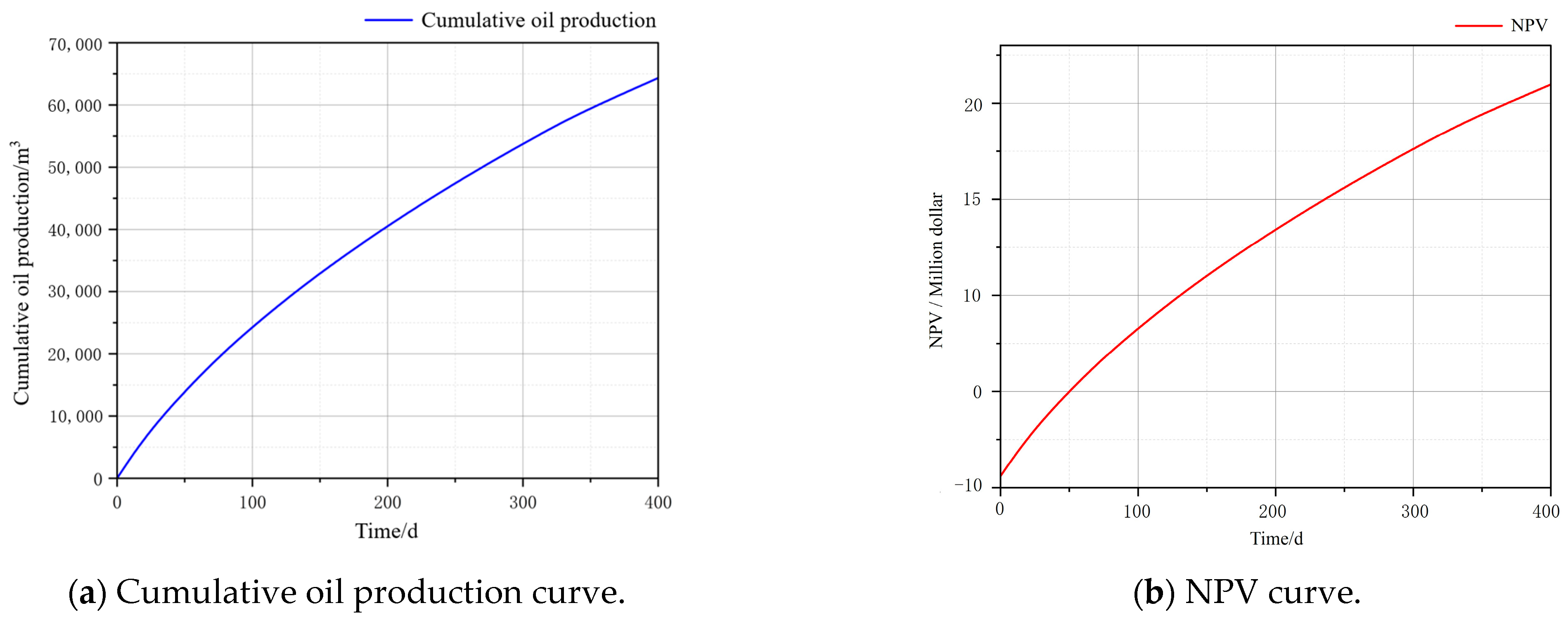
Using the reservoir parameters from the field case in Section 2.2, together with the NPV model and the economic parameters defined in Section 3.1, productivity prediction and economic evaluation were carried out over a 400-day production period. Based on the semi-analytical model, the cumulative oil production and NPV evolution for a complex-structured horizontal well were calculated, as shown in Figure 11.

At present, multi-stage fractured horizontal wells are relatively mature in offshore fields, whereas complex-structured multilateral fractured wells (e.g., fishbone wells) have attracted increasing attention in recent years but still lack sufficient field cases to support corresponding completion and optimization methods. To further assess the applicability of the proposed model and optimization method under complex well conditions and to broaden potential application scenarios, a hypothetical case of a fishbone-shaped multilateral fractured well was constructed while keeping the reservoir and economic parameters unchanged. Here, “fishbone” refers to a multilateral well configuration in which several branch wellbores extend from the main wellbore in a regular, rib-like pattern. This structured wellbore–fracture geometry is adopted here as an idealized engineering representation for model application and optimization analysis, rather than a direct description of irregular natural-fracture systems. Accordingly, the following fishbone-well optimization is presented as a demonstrative case study under assumed reservoir and economic conditions. The wellbore architecture and fracture distribution are shown in Figure 12, and the spatial configuration, completion staging, and fracture parameters of the main and branch wellbores are listed in

Table 5. Basic parameters of the fishbone-shaped multilateral fractured well.

Parameter	Value	Unit
Main wellbore length	1500	m
Branch wellbore length	500	m
Branch spacing	300	m
Branch angle	45	°
Wellbore position in x-direction (x0)	1500	m
Wellbore toe location in y-direction (y1)	750	m
Wellbore heel location in y-direction (y2)	2250	m
Wellbore position in z-direction (z0)	6.65	m
Number of stages per branch	3	/
Fracture half-length	95	m
Fracture width	0.01	m
Fracture conductivity	125	D·cm

.

4.3.1. Comparison Between a Fishbone Complex-Structured Well and a Complex-Structured Horizontal Well

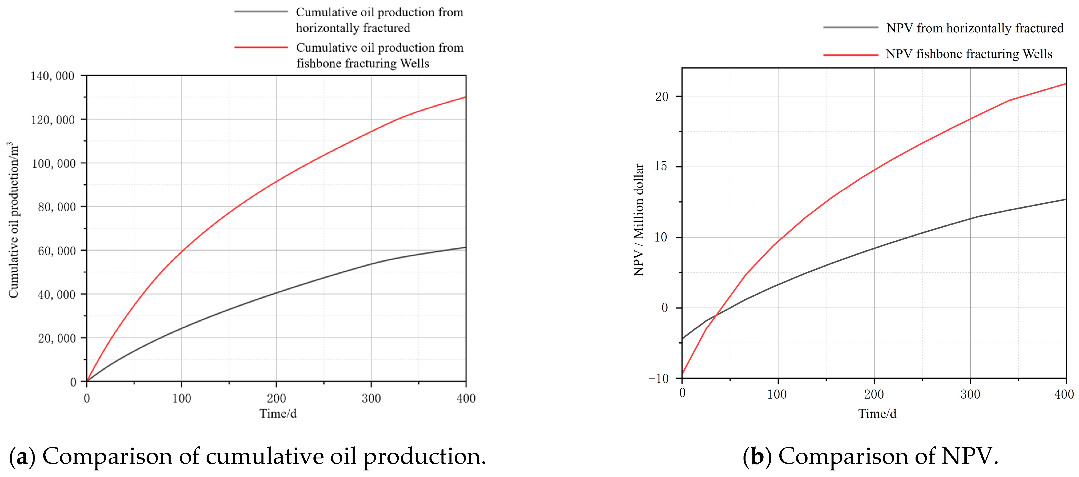
Using the parameters in Table 5, a semi-analytical model for a four-branch fishbone complex-structured well was established and simulated for 400 days. Its cumulative oil production and NPV were compared with those of a complex-structured multi-stage fractured horizontal well, with the results shown in Figure 13. For comparability, the fishbone well and the multi-stage fractured horizontal well are evaluated under the same reservoir parameters, production period, and economic conditions, while the main difference lies in the wellbore architecture and the associated completion/fracture configuration.

As indicated by the results, the four-branch fishbone complex-structured well involves more completion stages and a larger fracture scale, which increases well cost by approximately 6.81 million USD (about 48.7%). However, compared with the complex-structured multi-stage fractured horizontal well, the fishbone well greatly expands the effective drainage/contact area. Over 400 days, cumulative oil production increases by about 63,900 m³ (about 47.7%), and the resulting NPV increases by 20.97 million USD (about 46.7%). These results indicate that, for the constructed fishbone-well case under the assumed reservoir and economic conditions, the coupled workflow yields a numerically more favorable outcome than the compared fractured horizontal-well configuration.

4.3.2. Joint Optimization of Completion and Fracture Parameters for the Fishbone Complex-Structured Well

Based on the fishbone complex-structured well model described above, the joint optimization of completion parameters and fracture-geometry parameters was further conducted. Considering engineering feasibility, reasonable bounds and step sizes were specified for each variable. The parameter ranges are listed in

Table 6. Optimization parameter ranges.

Optimization Variable	Upper Bound	Lower Bound	Step Size
Number of stages per branch	8	1	1
Fracture half-length (m)	200	10	10
Stage spacing (m)	120	10	10
Fracture conductivity (D·cm)	300	100	25

.

To provide a basic computational justification for the GA-based optimization, the average wall-clock time for one forward model evaluation over the 400-day production period was tested on the implementation platform used in this study. The result shows that one evaluation requires approximately 1.3 s on average under the adopted discretization and solver settings. Under the present GA configuration of 80 individuals and 100 generations, the optimization requires approximately 8000 forward model evaluations, indicating that the semi-analytical model is computationally feasible for offline case-study optimization.

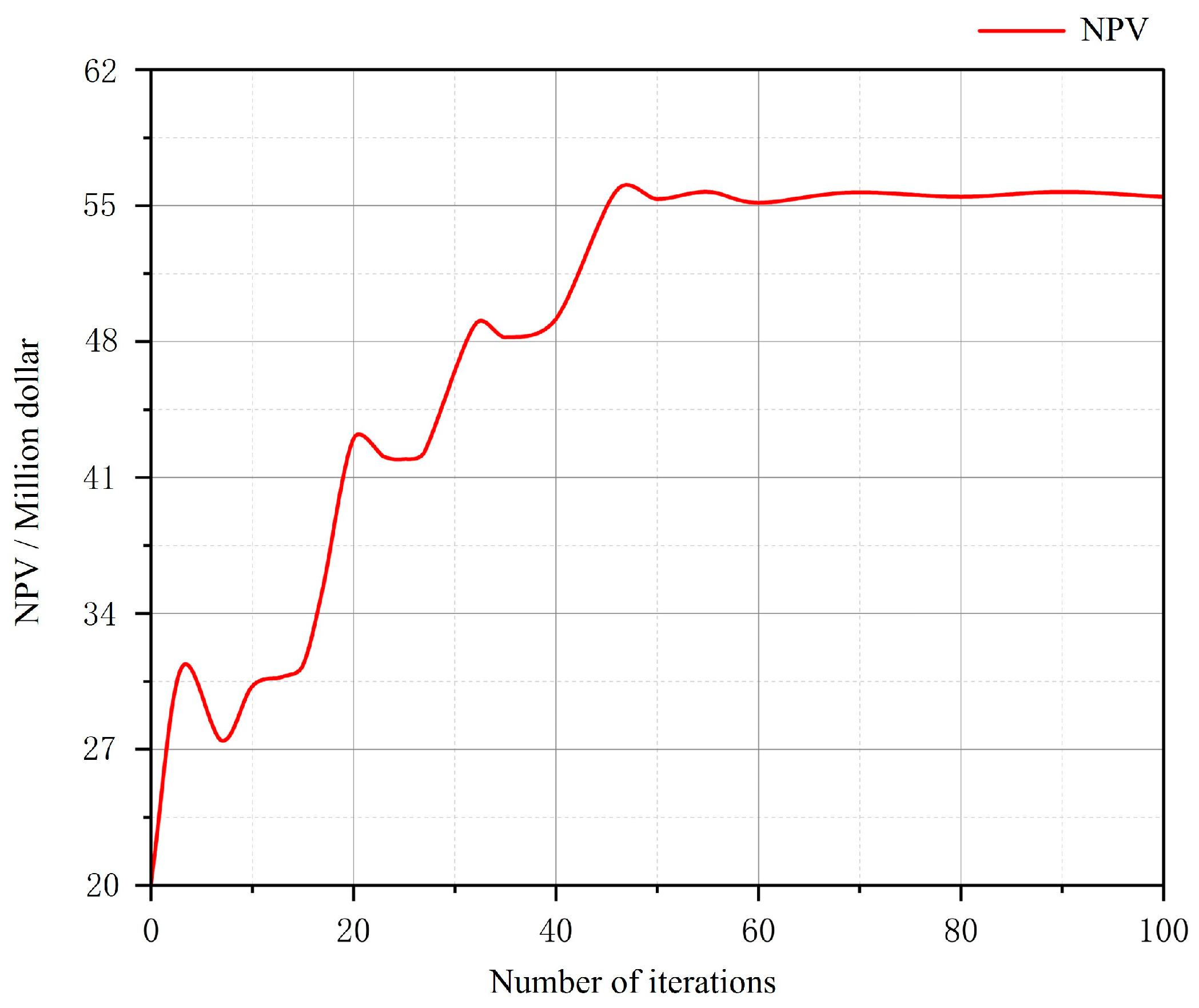
After encoding the completion and fracture parameters, the initial population is generated by the genetic algorithm. In the present implementation, binary encoding is adopted for the optimization variables. Each generation contains 80 individuals. The maximum number of iterations is set to 100, and the mutation rate is set to 0.1. Roulette-wheel selection is used to pass favorable genes to the next generation. New offspring are generated through two-point crossover and uniform mutation to enlarge the search range. For each individual, the optimization algorithm calls the semi-analytical productivity model to compute cumulative oil production at the day 400, and the NPV formula is used to calculate the fitness value. The updated population is then evaluated again by the productivity module in the next iteration. The optimization terminates when the preset maximum number of iterations is reached; otherwise, the above procedure is repeated. Accordingly, the reported solution represents the best individual obtained within the preset 100-generation search under the adopted GA settings. These parameter settings are adopted as the GA control parameters for the present case study. The convergence history for the four-branch fishbone well is shown in Figure 14.

As shown in Figure 15, the optimum NPV of 56.33 million USD is reached at the iteration 46. The corresponding optimal combination of completion staging parameters and fracture-geometry parameters is listed in

Table 7. Optimal parameter set.

Branch	Number of Stages	Fracture Half-Length (m)	Stage Spacing (m)	Conductivity (D·cm)
Branch 1	4	110	90	100
Branch 2	4	110	90	100
Branch 3	4	120	80	100
Branch 4	3	110	80	100

.

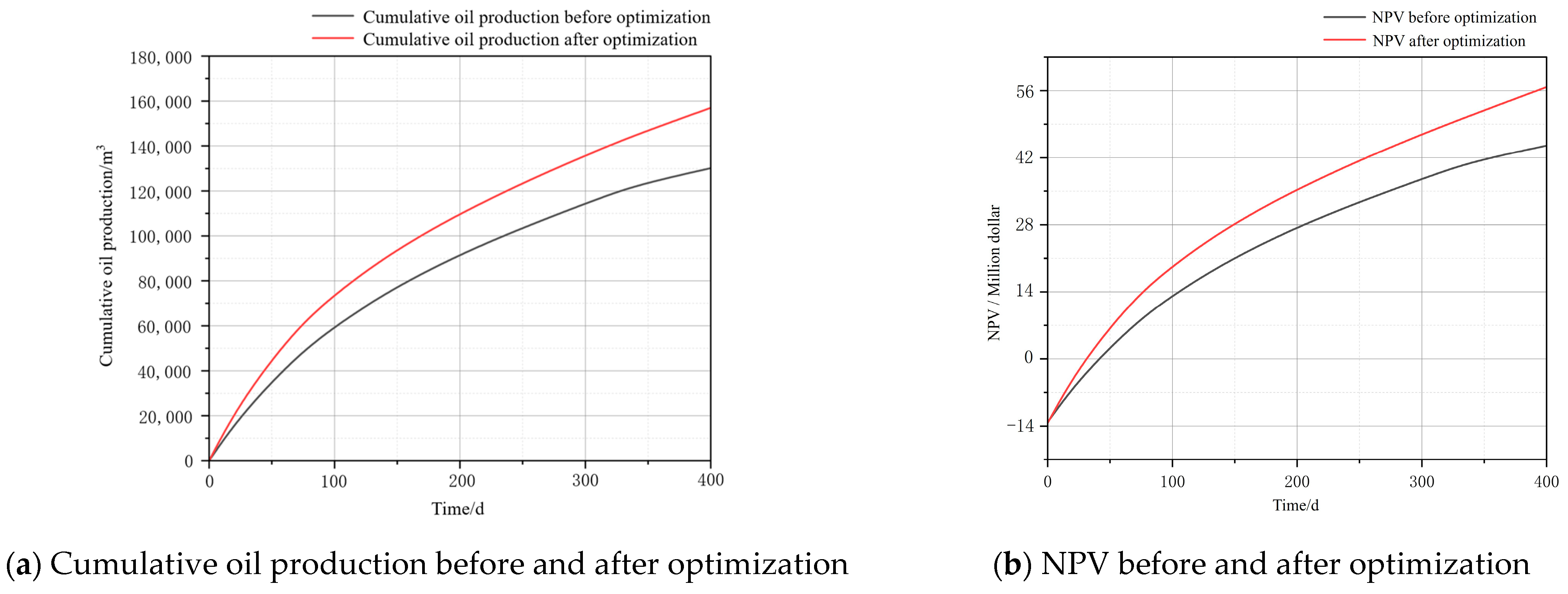
The optimal parameters in Table 7 were then used in the semi-analytical model to compare cumulative oil production and NPV before and after the optimization. The results are shown in Figure 15a,b.

The results show that, under the optimal parameter combination, the number of completion stages, fracture half-length, and stage spacing for each branch generally increase, whereas fracture conductivity reaches the lower bound of the tested range. This indicates that once the multibranch fractured architecture has significantly enhanced well–reservoir connectivity, further increasing fracture conductivity yields limited marginal production benefit, and the additional economic return cannot offset the increase in the fracturing cost. This also implies that, under the present reservoir and cost conditions, the optimization result is controlled by the balance between expanded drainage/contact area and the incremental cost of fracture treatment. In this sense, completion staging and fracture spacing play a more important role in improving overall economic performance than simply increasing conductivity. It should be noted that this result is obtained under the assumed parameter ranges, simplified cost model, and constructed fishbone-well case considered in the present study, and should therefore be interpreted as case-dependent rather than universally applicable.

With an increase in total cost of only about 0.153 million USD (approximately 1.2%), cumulative oil production increases by about 2.8 × 10⁴ m³ (approximately 17.7%), and NPV increases by about 11.25 million USD (approximately 20.2%). Here, the reported production and NPV improvements are measured relative to the initial completion and fracture parameters combination before optimization. These results indicate that, for the constructed fishbone-well case considered in this study, joint adjustment of completion staging and fracture parameters can lead to a more favorable economic outcome under the assumed reservoir and cost conditions. Accordingly, the reported 20.2% improvement reflects the relative change between the compared scenarios under the adopted empirical cost model and fixed economic assumptions, rather than a fully generalizable field-economic conclusion.

5. Discussion

The results show that the productivity and economic performance of complex-structured fractured wells are controlled by the coupled effects of reservoir flow, fracture flow, and wellbore flow. Under the studied low-permeability reservoir conditions, the fishbone-shaped multilateral fractured well provides a larger effective drainage/contact area and better well–reservoir connectivity than the conventional fractured horizontal well, leading to higher cumulative oil production and NPV [24,25,26,27]. In addition, the optimization results indicate that simply increasing fracture conductivity does not necessarily maximize economic benefit, because the marginal production gain may be insufficient to compensate for the added fracturing cost [28]. The convergence to the lower conductivity bound in the present case is mainly controlled by the adopted cost model and tested parameter range, and should therefore be interpreted as case-dependent. Although the branch-junction pressure-drop model is included in the coupled productivity calculation, its separate contribution to the final NPV has not been isolated in the present work and should be further assessed through on/off or coefficient-perturbation sensitivity analysis. In addition, the optimized branch-wise staging scheme should still be checked against actual drilling and completion operability before field implementation.

Compared with previous studies, which mainly focused on productivity prediction for specific well types or optimization of individual fracture parameters, the present work presents an engineering-oriented workflow that combines a coupled semi-analytical productivity model with NPV-oriented optimization for completion staging and fracture-geometry parameters [29]. The agreement with both the water–electric analogy experiments and the field case supports the applicability of the method under the studied conditions. Nevertheless, the present results are still case-dependent because the model is established under simplifying assumptions such as single-phase flow, constant fracture properties, and simplified economic correlations. Future work should further incorporate multiphase flow, time-dependent fracture behavior, and economic uncertainty [30], and validate the workflow using historical fishbone-well or multilateral fractured-well cases with available completion design, post-fracturing production, and cost records. Such validation would allow the workflow-recommended design to be compared with the implemented design in terms of production and NPV.

6. Conclusions

(1)

Based on the plane-source flow function for a box-shaped reservoir, the wellbore segments and equivalent inflow units were discretized to establish a coupled reservoir–fracture–wellbore semi-analytical productivity model for complex-structured wells. The model was validated through water–electric analogy experiments and a field case, confirming its rationality and applicability.

(2)

Building on the semi-analytical productivity model, an economic evaluation metric with NPV as the objective function was introduced. A joint optimization method for completion staging parameters and fracture-geometry parameters was established for complex-structured wells, and automatic parameter search was implemented using a genetic algorithm.

(3)

For the hypothetical fishbone-well case considered under the studied low-permeability reservoir and economic conditions, the optimized result tends toward more completion stages, larger fracture half-length, and lower fracture conductivity within the tested range. This result is presented as a case-specific demonstration of how geometric parameters, completion staging, branch-junction loss, and the adopted economic metric interact under the simplifying assumptions of the present study.

(4)

The results further indicate, for the present case, diminishing marginal returns in the economic benefit from simply enlarging fracture size or equivalent inflow capacity. Under the assumptions adopted in this study, completion-staging optimization appears to play a more influential role than simply increasing fracture conductivity. These findings, including the trend of reduced fracture conductivity and the observed diminishing-return behavior, are subject to the simplified assumptions adopted herein, namely single-phase flow, constant fracture properties, and simplified deterministic cost functions. Therefore, the low-conductivity tendency and diminishing-return conclusion should not be generalized to field design without further validation under more realistic conditions.

In practical offshore reservoir development, multiphase flow is often encountered, especially during medium- and late-stage production. The present model does not explicitly account for relative permeability, phase interference, fluid-property variation among phases, or the multiphase pressure-drop behavior in the wellbore. Therefore, its applicability under strong multiphase-flow conditions is limited. In addition, possible time-dependent changes in fracture conductivity are not considered, which may limit the applicability of the model under more complex production conditions. The economic objective is based on simplified empirical cost correlations under fixed economic conditions. In addition, the present optimization is deterministic and does not account for geological, economic, or operational uncertainties. Future work will focus on validating the present workflow using real-field data or a high-fidelity simulated pilot case, while also extending the framework by incorporating multiphase reservoir seepage, fracture-flow coupling, and multiphase wellbore flow models.

References

1. Tassone, G.; Giammancheri, M.; Banoori, S.; Parziale, S.; Mittiga, V.; Ilyasov, R.; Dupouy, N.; Reilly, B. Hydraulic fracturing challenges and solutions for the development of a low permeability oil reservoir—Case history from offshore west africa. In Proceedings of the SPE Conference at Oman Petroleum & Energy Show, Muscat, Oman, 21–23 March 2022. [Google Scholar] [CrossRef]
2. Almedallah, M.; Altaheini, S.K.; Clark, S.; Walsh, S. Combined stochastic and discrete simulation to optimise the economics of mixed single-horizontal and multilateral well offshore oil developments. Pet. Explor. Dev. 2021, 48, 1183–1197. [Google Scholar] [CrossRef]
3. Khosravanian, R.; Aadnøy, B.S. Well completion optimization by decision-making. In Methods for Petroleum Well Optimization; Gulf Professional Publishing: Houston, TX, USA, 2022. [Google Scholar] [CrossRef]
4. Li, L.; Xie, M.; Liu, W.; Dai, J.; Feng, S.; Luo, D.; Wang, K.; Gao, Y.; Huang, R. A new productivity evaluation method for horizontal wells in offshore low-permeability reservoir based on modified theoretical model. Processes 2024, 12, 2830. [Google Scholar] [CrossRef]
5. Syrtlanov, V.; Golovatskiy, Y.; Chistikov, K.; Bormashov, D. Experience in optimizing the location and parameters of multistage hydraulic fractures for a multilateral well based on reservoir simulation. In Proceedings of the SPE Russian Petroleum Technology Conference, Virtual, 12–15 October 2021. [Google Scholar] [CrossRef]
6. Yao, S.; Wang, X.; Yuan, Q.; Guo, Z.; Zeng, F. Production analysis of multifractured horizontal wells with composite models: Influence of complex heterogeneity. J. Hydrol. 2020, 583, 124542. [Google Scholar] [CrossRef]
7. Li, Z.; Wu, X.; Han, G.; Zhang, L.; Zhao, R.; Shi, S. A semi-analytical pressure model of horizontal well with complex networks in heterogeneous reservoirs. J. Pet. Sci. Eng. 2021, 202, 108511. [Google Scholar] [CrossRef]
8. Wang, W.; Fan, D.; Sheng, G.; Chen, Z.; Su, Y. A review of analytical and semi-analytical fluid flow models for ultra-tight hydrocarbon reservoirs. Fuel 2019, 256, 115737. [Google Scholar] [CrossRef]
9. Jia, P.; Cheng, L.; Huang, S.; Cao, R.; Xu, Z. A semi-analytical model for production simulation of complex fracture network in unconventional reservoirs. In Proceedings of the SPE/IATMI Asia Pacific Oil & Gas Conference and Exhibition, Nusa Dua, Indonesia, 20–22 October 2015. [Google Scholar] [CrossRef]
10. Sun, H.; Ouyang, W.; Zhu, S.; Wan, Y.; Tang, Y.; Cao, W. A new numerical well test method of multi-scale discrete fractured tight sandstone gas reservoirs and its application in the kelasu gas field of the tarim basin. Nat. Gas Ind. B 2023, 10, 103–113. [Google Scholar] [CrossRef]
11. Guo, J.; Zeng, F.; Zhao, J.; Xu, Y. A New Model to Predict Fractured Horizontal Well Production; OnePetro: Richardson, TX, USA, 2006. [Google Scholar]
12. Zhou, X.; Ran, Q. Optimization of fracturing parameters by modified genetic algorithm in shale gas reservoir. Energies 2023, 16, 2868. [Google Scholar] [CrossRef]
13. Wang, Y.; Liu, Y.; Sun, L. Optimization of reasonable production pressure difference of multiple-fractured horizontal well in fractured tight reservoir. Arab. J. Geosci. 2019, 12, 297. [Google Scholar] [CrossRef]
14. Hassan, A.; Elkatatny, S.; Abdulraheem, A. Application of artificial intelligence techniques to predict the well productivity of fishbone wells. Sustainability 2019, 11, 6083. [Google Scholar] [CrossRef]
15. He, J.; Zhang, Y.; Luo, E.; Xu, A.; Chen, Y.; Liu, Y.; Zeng, X.; Jiang, L. A coupling model of gas–water two-phase productivity for multilateral horizontal wells in a multilayer gas reservoir. Processes 2024, 12, 1643. [Google Scholar] [CrossRef]
16. Song, X.; Liu, Y.; Xue, L.; Wang, J.; Zhang, J.; Wang, J.; Jiang, L.; Cheng, Z. Time-series well performance prediction based on long short-term memory (LSTM) neural network model. J. Pet. Sci. Eng. 2020, 186, 106682. [Google Scholar] [CrossRef]
17. Meng, L.E.I.; Tianjun, Q.I.; Sheng, Y.I.N.; Chuanyun, Z.; Dan, L.I.; Xiaoyue, S.H.U.; Yang, L.U.O.; Haozhe, S.H.I. Optimizing shale-gas fracturing parameters in luzhou block based on random forests and particle swarm algorithm(RF-PSO). Nat. Gas Technol. Econ. 2023, 17, 53–61. [Google Scholar] [CrossRef]
18. Shu, J.; Han, G.; Yue, Z.; Cheng, L.; Dong, Y.; Liang, X. Optimizing Well Trajectories for Enhanced Oil Production in Naturally Fractured Reservoirs: Integrating Particle Swarm Optimization with an Innovative Semi-Analytical Model Framework. SPE J. 2025, 30, 957–975. [Google Scholar] [CrossRef]
19. Xu, Y.; Zhao, Y.; Xiang, Z.; Liang, H. A semi-analytical production prediction model of multi-stage fractured horizontal well rectangular heterogeneity gas reservoirs. Int. J. Heat Mass Transf. 2025, 236, 126238. [Google Scholar] [CrossRef]
20. Deng, J.; He, J.; Liu, J.; Song, H. Improved identification of fracture total factor characteristics and cross-scale flow channels by interpreting initial production data of horizontal wells. J. Clean. Prod. 2024, 450, 142005. [Google Scholar] [CrossRef]
21. Deng, J.; He, J.; Zhang, L.; Song, H.; Gao, L. Investigation into contributions of fracture geometry characterization and interference to productivity of multi-fractured vertical gas well. Gas Sci. Eng. 2024, 121, 205202. [Google Scholar] [CrossRef]
22. Penmatcha, V.R. Modeling of Horizontal Wells with Pressure Drop in the Well. Ph.D. Thesis, Stanford University, Stanford, CA, USA, 1997. [Google Scholar]
23. Stoten, D.P.; Benchoubane, H. The minimal control synthesis identification algorithm. Int. J. Control. 1993, 58, 685–696. [Google Scholar] [CrossRef]
24. Ai, K.; Duan, L.; Gao, H.; Jia, G. Hydraulic Fracturing Treatment Optimization for Low Permeability Reservoirs Based on Unified Fracture Design. Energies 2018, 11, 1720. [Google Scholar] [CrossRef]
25. Dong, Z.; Wu, L.; Wang, L.; Li, W.; Wang, Z.; Liu, Z. Optimization of Fracturing Parameters with Machine-Learning and Evolutionary Algorithm Methods. Energies 2022, 15, 6063. [Google Scholar] [CrossRef]
26. Wang, B.; Fang, Y.; Li, L.; Liu, Z. Automatic Optimization of Multi-Well Multi-Stage Fracturing Treatments Combining Geomechanical Simulation, Reservoir Simulation and Intelligent Algorithm. Processes 2023, 11, 1759. [Google Scholar] [CrossRef]
27. Jahandideh, A.; Jafarpour, B. Optimization of Hydraulic Fracturing Design under Spatially Variable Shale Fracability. J. Pet. Sci. Eng. 2016, 138, 174–188. [Google Scholar] [CrossRef]
28. Yang, X.; Guo, B.; Zhang, X. An Analytical Model for Capturing the Decline of Fracture Conductivity in the Tuscaloosa Marine Shale Trend from Production Data. Energies 2019, 12, 1938. [Google Scholar] [CrossRef]
29. Xiao, C.; Zhang, S.; Ma, X.; Zhou, T.; Li, X. Surrogate-Assisted Hydraulic Fracture Optimization Workflow with Applications for Shale Gas Reservoir Development: A Comparative Study of Machine Learning Models. Nat. Gas Ind. B 2022, 9, 219–231. [Google Scholar] [CrossRef]
30. Lin, Q.; Fang, W.; Zhang, L.; Mu, Q.; Li, H.; Li, L.; Wang, B. Robust Optimization of Hydraulic Fracturing Design for Oil and Gas Scientists to Develop Shale Oil Resources. Processes 2025, 13, 1920. [Google Scholar] [CrossRef]
Figure 1. Flow schematic of a box-shaped reservoir.
Processes 14 01762 g001
Figure 2. Schematic of fracture flow.
Processes 14 01762 g002
Figure 3. Schematic of wellbore pipe flow.
Processes 14 01762 g003
Figure 4. Schematic of a complex-structured well.
Processes 14 01762 g004
Figure 5. Simplified wellbore model at a branch-main confluence.
Processes 14 01762 g005
Figure 6. Water–electric analogy experimental setup for a fishbone-shaped multilateral complex-structured well.
Processes 14 01762 g006
Figure 7. Comparison between experimental production and semi-analytical model predictions for a complex-structured multilateral well.
Processes 14 01762 g007
Figure 8. Comparison between field production data and semi-analytical model results.
Processes 14 01762 g008
Figure 9. Schematic of a four-branch fishbone complex-structured well.
Processes 14 01762 g009
Figure 10. Encoding scheme for completion and fracture parameters of a four-branch fishbone complex-structured well.
Processes 14 01762 g010
Figure 11. Cumulative oil production and NPV curves for a complex-structured horizontal well.
Processes 14 01762 g011
Figure 12. Schematic of the wellbore and fractures for a fishbone-shaped complex-structured well.
Processes 14 01762 g012
Figure 13. Comparison of production and economic performance between a fishbone fractured well and a multi-stage fractured horizontal well.
Processes 14 01762 g013
Figure 14. Convergence history of the genetic algorithm for completion and fracture parameter optimization.
Processes 14 01762 g014
Figure 15. Comparison of cumulative oil production and NPV before and after optimization.
Processes 14 01762 g015