Industrial Process Monitoring Based on DiPCA and ARMA-Transformer

Abstract

This study addresses the problem of incipient fault detection in industrial processes by developing an enhanced dynamic inner principal component analysis (DiPCA) framework. This framework integrates a Transformer attention mechanism and a masked linear autoregressive moving average (ARMA) structure. In contrast to the original DiPCA, this approach can effectively characterize complex dynamic processes while maintaining the theoretical integrity of the original framework. Here, the sliding-window singular value decomposition is chosen to construct the dynamic feature matrix. The ARMA-Transformer network can capture the multi-step prediction features. A DiPCA-based dual monitoring system can then be used to establish dynamic and static residual statistics. The simulations of the Tennessee Eastman Process (TEP) demonstrate that the proposed method yields fault detection rates (FDRs) of 77.80% and 69.50% for incipient faults 3 and 9. These are higher than those of traditional DiPCA, ARMA, PCA, and DPCA by more than 40% on average. Validation on the Case Western Reserve University (CWRU) bearing dataset further shows an average FDR of 94.74% across 13 fault conditions. It thus offers an effective approach for early anomaly identification and safety monitoring in complex industrial processes.

1. Introduction

Fault detection plays a fundamental role in ensuring the safety and efficiency of industrial processes. Modern industrial systems are becoming increasingly complex. Therefore, the early and accurate detection of incipient faults is essential. These faults usually have subtle amplitudes and evolve slowly. If such faults remain undetected, they may progressively accumulate, leading to severe production disruptions and economic losses. Consequently, reliable and real-time fault detection technologies are required. These technologies must also handle noise and complex process dynamics effectively.

Over the past decades, numerous data-driven methods have been proposed for process monitoring. Principal component analysis (PCA) [1], Partial Least Squares (PLS) [2], and Independent Component Analysis (ICA) [3] represent foundational approaches. However, they rely on linear and static assumptions. These methods ignore temporal dependencies and cannot capture the gradual evolution of incipient faults. To address dynamics, extensions such as Dynamic PCA (DPCA) [4] and Dynamic PLS (DPLS) [5] were developed. They incorporate time-lagged variables but remain fundamentally linear, and the augmented dimensionality grows rapidly with lag order. This curse of dimensionality is compounded by the fact that these methods offer no remedy for nonlinear process behaviors. Nonlinear variants, including Kernel PCA (KPCA) [6] and Kernel PLS (KPLS) [7], map data into high-dimensional feature spaces to capture nonlinearities. Nevertheless, they still struggle with incipient faults whose weak amplitudes are easily masked by noise and normal variations. Moreover, quality-driven methods like PLS and its variants introduce additional detection delays due to their reliance on the availability and timeliness of quality measurements, which is particularly unsuitable for early fault scenarios. Collectively, despite these methodological advances from linear static to dynamic and nonlinear frameworks, existing approaches still fall short of providing reliable detection for incipient faults.

Deep learning methods have also been applied to process monitoring. Convolutional Neural Networks (CNNs) [8] effectively extract local features from raw data. Stacked Autoencoders (SAEs) [9] and their variants, such as Deep Ensemble SAE (DE-SAE) [10], excel at nonlinear dimensionality reduction. However, their reconstruction objectives are mainly static. This limits their capacity to model dynamic evolution patterns. More recently, the Transformer architecture [11] has gained attention. Its self-attention mechanism can capture long-range dependencies and overcomes the vanishing gradient limitations of Recurrent Neural Networks (RNNs) [12]. Subsequent studies have further integrated attention mechanisms with Long Short-Term Memory (LSTM) [13] to enhance the identification of critical time steps. Nevertheless, applying standard Transformer architectures to industrial process monitoring remains non-trivial: industrial data exhibit strong autocorrelation and high noise levels, which differ fundamentally from the linguistic data for which Transformers were originally designed. Given these limitations, deep learning methods alone are often insufficient for detecting subtle incipient faults.

Recent research has explored hybrid methods that integrate statistical and deep learning paradigms. These methods combine the interpretability of traditional multivariate statistical process monitoring (MSPM) techniques with the representational power of deep neural networks. These efforts span three primary directions.

The first focuses on ensemble learning frameworks that fuse multiple detectors or features, progressing from a PCA ensemble detector (PCAED) [14] for detecting specific incipient faults, to a time-domain Feature Ensemble Net (FENet) [15], and further to a dense FENet [16] that integrates multiple basic detectors and a time/frequency feature-driven ensemble method [17] that combines time-domain FENet with a PSD-based frequency-domain network via Bayesian inference.

The second direction introduces statistical testing on network outputs to enhance detection reliability. Representative works include a hybrid framework combining ANN-based classification with sequential hypothesis testing for parameter change detection in power converters [18], a system integrating deep anomaly detection with sequential probability ratio testing for temporal evidence aggregation [19], and a method that couples significance testing with conformal prediction to construct prediction sets with formal risk guarantees for fault detection [20]. A third direction combines DiPCA [21] with recurrent networks such as LSTM for dynamic process monitoring [22]. While effective, this approach treats the neural network as an external predictor applied after DiPCA. The proposed method differs in that the ARMA [23]-Transformer replaces the linear AR component inside DiPCA, preserving the autoregressive form, the unsupervised learning setting, and the statistical interpretability of the DiPCA framework. Despite these advances, a closer examination reveals a fundamental distinction: the neural network and the statistical component are coupled externally—operating either as parallel detection modules in ensemble frameworks, or as post hoc decision layers in reliability-oriented approaches. This external coupling limits how organically the neural network can be integrated with the statistical decomposition and residual analysis that underpin traditional MSPM frameworks.

In this work, we explore a distinct architectural paradigm: embedding an ARMA-Transformer directly as the dynamic engine inside DiPCA, replacing its original linear autoregressive component while preserving the full DiPCA statistical backbone. Unlike external coupling, the neural network becomes an integral part of the MSPM framework. This deep integration enables the network’s nonlinear dynamic modeling capability to directly enhance the latent variables extraction that is central to DiPCA, while the established statistical mechanisms of DiPCA remain intact to ensure reliable fault detection decisions. The main contributions of the proposed method are listed as follows:

(1)

A new architecture is proposed that integrates deep learning with traditional statistical process monitoring, offering an effective solution for industrial process safety monitoring. Traditional statistical methods like DiPCA are interpretable and provide rigorous control limits, but their linear dynamics cannot capture complex nonlinear patterns in modern industrial processes. Deep learning methods like Transformers excel at nonlinear modeling, but they lack statistical inferential power and are difficult to interpret. The proposed architecture combines the strengths of both: the ARMA-Transformer handles nonlinear dynamic prediction, while DiPCA provides the statistical framework for residual analysis and fault decision.

(2)

The novelty lies in embedding a neural network as the dynamic core inside DiPCA, rather than adding it as an external module. The original DiPCA relies on a linear autoregressive model to capture temporal dependencies. In this work, an AR-MA-Transformer takes over this role at the same position, while the projection matrices, residual deflation, and control limit calculation of DiPCA remain unchanged. The neural network is not added as an external module; it is placed inside DiPCA as its dynamic engine.

The remainder of this paper is organized as follows. Section 2 gives the problem formulation. Section 3 introduces the details of the proposed ARMA-Transformer DiPCA framework. Section 4 presents experimental results and analysis on the Tennessee Eastman Process (TEP) [24] and the Case Western Reserve University (CWRU) [25] bearing dataset. Finally, Section 5 and Section 6 summarize findings and discuss future work.

2. Problem Formulation

Despite extensive research on fault detection in industrial processes, the reliable detection of incipient faults under unsupervised conditions remains a significant challenge. These faults are typically characterized by their small amplitude and susceptibility to process noise and operating fluctuations. In addition, their fault features often manifest only in a subset of process variables. Unlike abrupt faults that produce sustained large deviations, incipient faults evolve slowly with amplitudes comparable to normal process variations, making them statistically indistinguishable from normal behavior when examined on a per-sample basis.

Existing methods such as DiPCA have demonstrated effectiveness in dynamic process monitoring. However, the linear autoregressive component at the core of DiPCA inherently limits its sensitivity to the subtle, nonlinear evolution patterns of incipient faults in complex industrial environments. This limitation becomes particularly pronounced under unsupervised conditions without labeled fault data.

To address this critical limitation, an enhanced DiPCA framework is proposed in this paper. Compared to traditional DiPCA, the proposed method introduces two key innovations: sliding-window singular value decomposition for dynamic feature extraction, and a masked linear ARMA attention model that replaces the linear dynamic component to generate more informative dynamic residuals. By combining residual analysis with multi-index thresholds and fusion rules, and determining control limits via kernel density estimation (KDE) [26], the framework achieves improved detection performance and numerical robustness, particularly for faults 3 and 9 in the TEP, as well as on the CWRU bearing dataset. It should be noted that simply appending deep learning models as external modules to an MSPM framework does not resolve the fundamental limitation. The linear dynamic component of DiPCA remains unchanged, and the statistical decomposition and residual analysis that define the monitoring backbone are not directly influenced by the deep learning component. A more effective approach is to replace the linear dynamic core of DiPCA with a neural network that serves as its internal dynamic engine, allowing the nonlinear modeling capacity to directly participate in the latent variables extraction and residual generation that are central to fault detection.

3. ARMA-Transformer Based on DiPCA

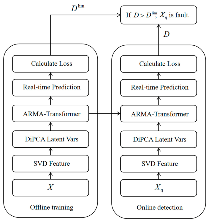
In this section, we describe how the proposed ARMA-Transformer based on DiPCA was developed. First, the dynamic latent variables were extracted through DiPCA. Then, sliding-window singular-value sequences were utilized to construct the features. Furthermore, an autoregressive Transformer with masked linear ARMA components was employed for multi-step forecasting. The overall framework of the proposed ARMA-Transformer based on DiPCA is illustrated in Figure 1.

3.1. Sliding-Window Singular Values

For the real-time data stream of industrial processes, set an appropriate window size $w$, and select $w-1$ samples immediately preceding the current sample to form a sliding-window matrix. Assume the sampling instant is $q$, and the number of sensors is $m$. Hence, the sliding-window matrix is given by

$$X_q=\left[\begin{array}{ccc}{x}_{q-w+1,1}& \dots & x_{q-w+1,m}\\ ⋮& \ddots & ⋮\\ x_{q,1}& \dots & x_{q,m}\end{array}\right]\in {\mathbb{R}}^{w\times m}$$

(1)

The standardization of $X_q$ yields the matrix ${\overline{\mathrm{X}}}_{\mathrm{q}}$:

$${\overline{\mathrm{X}}}_{\mathrm{q}}={\displaystyle \frac{X_q-1_{w\times 1}\times {\mathrm{\mu }}_q^T}{1_{w\times 1}\times {\sigma }_q^T}}$$

(2)

where $1_{w\times 1}$ denotes a column vector of ones, ${\mathrm{\mu }}_q\in {\mathbb{R}}^{1\times m}$ and ${\mathrm{\sigma }}_q\in {\mathbb{R}}^{1\times m}$ are row vectors of column-wise means and standard deviations:

$${\mathrm{\mu }}_q={\displaystyle \frac{1}{w}}{\sum }_{i=1}^W{X}_{q,i}$$

(3)

$${\mathrm{\sigma }}_{\mathrm{q}}=\sqrt{{\displaystyle \frac{1}{\mathrm{w}}}{\sum }_{\mathrm{i}=1}^{\mathrm{w}}{\left({\mathrm{X}}_{\mathrm{q},\mathrm{i}}-{\mu }_q\right)}^2}$$

(4)

where ${\mathrm{X}}_{\mathrm{q},\mathrm{i}}$ is the i-th row of $X_q$. After standardization, each column of ${\overline{\mathrm{X}}}_{\mathrm{q}}$ has zero mean and unit variance.

Performing singular value decomposition on the standardized sliding-window matrix $X_q\in {\mathbb{R}}^{w\times m}$ yields

$${\overline{\mathrm{X}}}_q={\mathrm{U}}_{\mathrm{q}}{\mathrm{M}}_{\mathrm{q}}{\mathrm{V}}_{\mathrm{q}}^{\mathrm{T}}$$

(5)

where $U_q\in {\mathbb{R}}^{w\times w}$ and $V_q\in {\mathbb{R}}^{m\times m}$ are orthogonal, and the diagonal entries of $M_q$ are the $m$ non-negative singular values $\left[{\mathrm{\sigma }}_{1,q},{\mathrm{\sigma }}_{2,q},\dots ,{\mathrm{\sigma }}_{m,q}\right]$ at time index $q$. By sliding the window along the time series, we collect, for each $j=1,2,\dots ,m$, the sequence

$$s_j={\left[{\mathrm{\sigma }}_{j,w},{\mathrm{\sigma }}_{j,w+1},\dots ,{\mathrm{\sigma }}_{j,T}\right]}^T$$

(6)

forming $m$ singular-value time series. Selecting the top $n_{sv}$ of these yields a multivariate sequence $S\in {\mathbb{R}}^{T^{\prime }\times n_{sv}}$ which serves as the input to the DiPCA stage. In this work, $n_{sv}=5$ is used. These singular value sequences compactly represent the dominant energy structure within each window. DiPCA is then applied to extract latent variables that exhibit strong temporal autocorrelation from this representation.

3.2. DiPCA

DiPCA integrates dynamic data modeling with PCA to extract latent variables with autocorrelation structures from high-dimensional process data.

In the dynamic latent variables extraction stage, it iteratively extracts $l$ dynamic latent variables $t_k=S{w}_k\left(k=1,2,\dots ,l\right)$, where $t_k\in {\mathbb{R}}^N$ represents the $k$-th latent variable scores and $w_k\in {\mathbb{R}}^{n_{sv}}$ is the $k$-th projection vector. The projection vector $w_k$ is obtained by solving the optimization problem:

$$\underset{w_k,\beta }{max}J={\sum }_{i=s}^{N-1}({\sum }_{j=1}^s{\beta }_j{t}_{k,i-j})t_{k,i}$$

(7)

subject to the constraints $\parallel w_k\parallel =1$ and $\parallel \beta \parallel =1$, where $s$ is the lag order, $\beta \in {\mathbb{R}}^s$ is the autoregressive coefficient vector, and $t_{k,i}=S_i{w}_k$ is the $i$-th score of the $k$-th component, where $S_i$ denotes the i-th row of the singular value feature matrix S

The optimization is solved iteratively through alternating updates. With $w_k$ fixed, $\beta$ is obtained by solving the least squares problem:

$$\beta =(T_{lag}^T{T}_{lag}{)}^{-1}{T}_{lag}^T{t}_{s+1:N}$$

(8)

and then normalized as $\beta \leftarrow \beta /\parallel \mathrm{\beta }\parallel$. Then, with $\beta$ fixed, $w_k$ is updated via gradient ascent followed by normalization, where the gradient is given by

$${\nabla }_{w_k}J=X^T\left(T_{\mathrm{lag}}\beta \right)+{\sum }_{j=1}^s{\beta }_j{X}_{s-j:N-1-j}^T{t}_{s+1:N}$$

(9)

This process iterates until convergence is achieved by monitoring relative changes in $w_k$ and $\beta$. Upon convergence, the loading vector is computed as

$$p_k={\displaystyle \frac{S^T{t}_k}{t_k^T{t}_k}}$$

(10)

and the residual matrix is updated by removing the extracted component:

$$S\leftarrow S-t_k{p}_k^T$$

(11)

In the Projection and Reconstruction Matrices stage, the final projection and loading matrices are

$$W=\left[w_1,w_2,\dots ,w_l\right]\in {\mathbb{R}}^{n_{sv}\times l}$$

(12)

$$P=\left[p_1,p_2,\dots ,p_l\right]\in {\mathbb{R}}^{n_{sv}\times l}$$

(13)

The latent variables and data reconstruction are given by

$$T=SR$$

(14)

$$\widehat{X}=T{P}^T$$

(15)

where $R=W(P^{T}W{)}^{-1}\in {\mathbb{R}}^{n_{sv}\times l}$ is the projection matrix.

3.3. Dynamic Prediction with ARMA Attention Formulation

The latent variables T extracted by DiPCA capture the dominant autocorrelated dynamics of the process, but the linear AR model within DiPCA cannot fully characterize the residual nonlinear temporal patterns. To address this, the dynamic prediction of latent variables employs an ARMA attention mechanism that integrates both autoregressive (AR) and moving average (MA) components. For the latent variables $T\in {\mathbb{R}}^{N\times l}$ obtained from DiPCA via Equation (14), the autoregressive component follows the AR structure of the classical ARMA model, where past observations are weighted by fixed coefficients:

$$o_t^{\mathrm{AR}}={\sum }_{i=1}^t{w}_{t,i}\odot v_i$$

(16)

where $v_i\in {\mathbb{R}}^{l\times d}$ represents the value vector at time $i$, and $w_{t,i}\in {\mathbb{R}}^{l\times d}$ denotes the attention weights derived from fixed parameter matrices rather than dynamic query–key interactions. This formulation constitutes a causal linear layer with a strictly lower triangular structure.

Following the moving average structure of the ARMA model, the prediction error is decomposed into past innovations weighted by MA coefficients:

$$v_{t+1}=o_t^{\mathrm{AR}}+o_t^{\mathrm{MA}}+{\mathrm{ϵ}}_t={\sum }_{i=1}^t{w}_{t,i}\odot v_i+{\sum }_{j=1}^{t-1}{\mathrm{\theta }}_{t-1,j}\odot {\mathrm{ϵ}}_j+{\mathrm{ϵ}}_t$$

(17)

where the AR residual term $r_t$ is decomposed as

$$r_t={\sum }_{j=1}^{t-1}{\mathrm{\theta }}_{t-1,j}\odot {\mathrm{ϵ}}_j+{\mathrm{ϵ}}_t$$

(18)

In the indirect MA weight generation stage, to avoid computationally expensive matrix operations while maintaining the MA structure, an indirect weight generation scheme is employed [27]. Instead of explicitly computing ${\mathrm{\theta }}_{t-1,j}$, the AR residuals $r_j$ are utilized as value inputs for the MA component:

$${\sum }_{j=1}^{t-1}{\mathrm{\beta }}_{t-1,j}\circ r_j={\sum }_{j=1}^{t-1}{\mathrm{\theta }}_{t-1,j}\circ {\mathrm{ϵ}}_j$$

(19)

This establishes the matrix relationship $Br=\mathrm{\Theta }ϵ$ with the implicit transformation:

$$B=\mathrm{\Theta }\cdot {\left(I+\mathrm{\Theta }\right)}^{-1}$$

(20)

$$\mathrm{\Theta }=B\cdot {\left(I-B\right)}^{-1}$$

(21)

The MA weight matrix $\mathrm{\Theta }$ exhibits desirable temporal decay properties, with elements satisfying

$${\mathrm{\theta }}_{ij}=b{\left(1+b\right)}^{i-j-1},\hspace{1em}\mathrm{for} i>j$$

(22)

where $b$ represents the characteristic decay parameter. This decay pattern matches the behavior of a standard MA process, where the influence of past innovations diminishes with increasing time lag.

In the MA component via the Transformed Queries and Keys stage, the MA component $o_t^{\mathrm{MA}}$ is computed using a dedicated attention mechanism applied to the AR residuals. First, the queries and keys for the MA part are transformed via specialized functions:

$$\widetilde{Q_t^{\mathrm{MA}}}={\mathrm{\varphi }}_q^{\mathrm{MA}}\left(Q_t^{\mathrm{MA}}\right)$$

(23)

$$\widetilde{K_j^{\mathrm{MA}}}={\mathrm{\varphi }}_k^{\mathrm{MA}}\left(K_j^{\mathrm{MA}}\right)$$

(24)

where ${\mathrm{\varphi }}_q^{\mathrm{MA}}$ and ${\mathrm{\varphi }}_k^{\mathrm{MA}}$ are element-wise transformation functions designed to shape the distribution of attention weights for the MA dynamics. The MA output is then obtained by applying the transformed attention weights to the residual values $r_j$:

$$o_t^{\mathrm{MA}}={\sum }_{j=1}^{t-1}\left({\displaystyle \frac{\widetilde{Q_t^{\mathrm{MA}}}{\left(\widetilde{K_j^{\mathrm{MA}}}\right)}^{\mathrm{\top }}}{\sqrt{d_k}}}\right)r_j$$

(25)

This formulation efficiently captures the short-term dependencies and error corrections in the residual sequence, corresponding to the MA characteristic within the attention framework.

In the final ARMA output and prediction stage, the final output of the ARMA attention block is generated by integrating the autoregressive and MA components, followed by a linear projection:

$$o_t=\left(o_t^{\mathrm{AR}}+o_t^{\mathrm{MA}}\right)W_o$$

(26)

where $W_o\in {\mathbb{R}}^{d\times d}$ is a learnable output projection matrix. This combined output $o_t$ serves as the one-step-ahead prediction for the latent variable scores at time $t+1$, effectively leveraging both the historical pattern (via AR) and the recent innovation sequence (via MA) to enhance dynamic prediction accuracy.

3.4. Control Limit Calculation and Fault Diagnosis

Once the ARMA-Transformer predicts the latent scores, the prediction error is decomposed into two complementary components: the dynamic residual in the latent space and the static residual in the original feature space. These residuals form the basis for fault detection. The control limits for monitoring statistics are established through KDE to characterize the empirical distribution of normal operation data. For each of the three monitoring statistics, the corresponding control limit ${\varphi }_{lim}$ is determined as the $\mathrm{\alpha }$-quantile of the KDE-fitted distribution. The KDE-based probability density function is formulated as

$$f_{\mathrm{KDE}}\left(x\right)={\displaystyle \frac{1}{nh}}{\sum }_{i=1}^{n}K\left({\displaystyle \frac{x-{\mathrm{\varphi }}_i}{h}}\right)$$

(27)

where $K\left(\cdot \right)$ is the Gaussian kernel function, $h$ is the bandwidth parameter, and ${\mathrm{\varphi }}_i$ are the observed monitoring statistics from normal operation data.

Three monitoring statistics are employed for comprehensive fault detection:

$${\mathrm{\varphi }}_v\left[i\right]=v{\left[i\right]}^T{\mathrm{\Sigma }}_v^{-1}v\left[i\right]$$

(28)

where $v\left[i\right]=T\left[i\right]-\widehat{T}\left[i\right]$ represents the dynamic residual vector.

$$T_r^2\left[i\right]=E_r{\left[i\right]}^T{\mathrm{\Sigma }}_r^{-1}{E}_r\left[i\right]$$

(29)

where $E_r\left[i\right]$ denotes the PCA-reduced static residual.

$$Q_r\left[i\right]=|\mathrm{E}\left[i\right]-\widehat{E}\left[i\right]{|}_2^2$$

(30)

where $E\left[i\right]=X\left[i\right]-\widehat{T}\left[i\right]P^T$ represents the static residual vector.

A process observation is flagged as faulty when any monitoring statistic exceeds its control limit.

3.5. Algorithms

The operation of the ARMA-Transformer based on DiPCA consists of two sequential parts. First, historical normal data is used to train the model and compute statistical control limits, as formalized in Algorithm 1. Subsequently, the trained model is deployed for continuous, real-time incipient fault detection on new data samples, with the exact steps provided in Algorithm 2.

Algorithm 1. Offline Training

Input: ${\mathrm{X}}_q$—input data; w—sliding window width; $n_{sv}$—number of singular values; s—lag order; l—number of latent variables

Output: P,W,R—DiPCA matrices; $w_{t,i}, {\mathrm{\beta }}_{t-1,j}, W_o$—trained parameters; ${\mathrm{\varphi }}_{\mathrm{v}}^{\mathrm{l}\mathrm{i}\mathrm{m}}$, ${{\mathrm{T}}^2}_{\mathrm{r}}^{\mathrm{l}\mathrm{i}\mathrm{m}}$, ${\mathrm{Q}}_{\mathrm{r}}^{\mathrm{l}\mathrm{i}\mathrm{m}}$—control limits

1: Normalize sliding windows

2: Perform SVD on each window and obtain sequence {$s_j$}, retain top $n_{sv}$ to form S 3: Extract l dynamic latent variables T and obtain P, W (Equations (7)–(11)) 4: Compute R (Equations (14) and (15))

5: for each training epoch do

6:   Input T into transformer

7:   Compute loss between predicted and actual T (Equations (16)–(26))

8:   Backpropagate loss and update model parameters $w_{t,i},{\mathrm{\beta }}_{t-1,j},W_o$ 9: end for 10: Perform forward pass on T to obtain predicted

11: Compute ${\mathrm{\varphi }}_v$, $T_r^2$, $Q_r$ on normal data (Equations (28)–(30))

12: Compute control limit ${\varphi }_v^{lim}$, ${T^2}_r^{lim}$, $Q_r^{lim}$ (Equation (27))

15: return P, W, R, $w_{t,i}, {\mathrm{\beta }}_{t-1,j}, W_o$, ${\mathrm{\varphi }}_{\mathrm{v}}^{\mathrm{l}\mathrm{i}\mathrm{m}}$, ${{\mathrm{T}}^2}_{\mathrm{r}}^{\mathrm{l}\mathrm{i}\mathrm{m}}$, ${\mathrm{Q}}_{\mathrm{r}}^{\mathrm{l}\mathrm{i}\mathrm{m}}$

Algorithm 2. Online Detection

Input: ${\mathrm{X}}_q$—new sample; P, W, R, $w_{t,i}, {\mathrm{\beta }}_{t-1,j}, W_o$, ${\mathrm{\varphi }}_{\mathrm{v}}^{\mathrm{l}\mathrm{i}\mathrm{m}}$, ${{\mathrm{T}}^2}_{\mathrm{r}}^{\mathrm{l}\mathrm{i}\mathrm{m}}$, ${\mathrm{Q}}_{\mathrm{r}}^{\mathrm{l}\mathrm{i}\mathrm{m}}$—trained parameters; s—lag order; ${\mathrm{\varphi }}_{\mathrm{v}}^{\mathrm{l}\mathrm{i}\mathrm{m}}$, ${{\mathrm{T}}^2}_{\mathrm{r}}^{\mathrm{l}\mathrm{i}\mathrm{m}}$, ${\mathrm{Q}}_{\mathrm{r}}^{\mathrm{l}\mathrm{i}\mathrm{m}}$—control limits

Output: status of ${\mathrm{X}}_q$

1: Extract singular values from sliding window on ${\mathrm{X}}_q$, perform SVD, form S

2: Project to latent space T (Equation (14))

3: for each predicted step do 4:  Predict T (Equations (16)–(26))

5:  Compute ${\mathrm{\varphi }}_v$, $T_r^2$, $Q_r$ (Equations (28)−(30))

6:  if ${\mathrm{\varphi }}_v>{\mathrm{\varphi }}_{\mathrm{v}}^{\mathrm{l}\mathrm{i}\mathrm{m}}$ or $T_r^2>{{\mathrm{T}}^2}_{\mathrm{r}}^{\mathrm{l}\mathrm{i}\mathrm{m}}$ or $Q_r>{\mathrm{Q}}_{\mathrm{r}}^{\mathrm{l}\mathrm{i}\mathrm{m}}$ then

7:   Mark step as abnormal

8:  else

9:   Mark step as normal

10:  end if

11: end for

12: if any abnormal step exists then

13:  status = fault

14: else

15:  status = normal 16: end if 17: return status of ${\mathrm{X}}_q$

4. Simulation

In this section, the famous benchmark TEP and the CWRU bearing dataset are used to verify the superior performance of the proposed methodology.

4.1. Tennessee Eastman Process

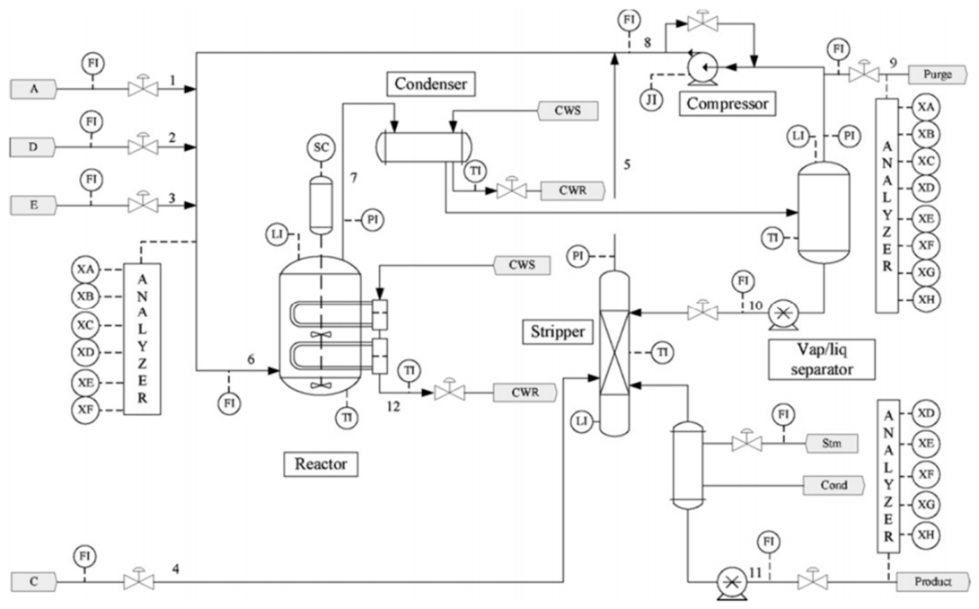
This chemical plant simulator, originally created at Eastman Chemical Company, is widely accepted in process systems engineering for benchmarking fault detection algorithms because it exhibits pronounced nonlinear and time-varying behavior. The simulation integrates five-unit operations: a reactor, product condenser, vapor–liquid separator, recycle compressor, and stripper. Thirty-three signals are logged: twenty-two continuous measurements (XMEAS 1–22) and eleven controller outputs (XMV 1–11). Together, they describe the essential dynamic and operational states of the plant. Twenty-one fault scenarios are predefined within the simulator. In this study, faults 3 and 9 are mainly examined. Fault 3 is a step change in the reactor cooling-water inlet temperature, and fault 9 is a random variation in the reactor feed composition. Figure 2 shows the system structure of TEP.

The simulation data were generated using a closed-loop version of the TEP [28], available at http://depts.Washington.edu/control/LARRY/TE/download.html (accessed on 10 April 2026). Both the training and test datasets were simulated for 200 h with a sampling interval of three minutes. For each test dataset, a fault was introduced after 100 h of simulation. With the exception of fault 6, 4000 training samples and 4000 faulty test samples were obtained for each fault type. It should be noted that fault 0 represents the normal operating condition. The fault detection rate (FDR) was calculated based on the last 2000 sampling instants of each test dataset, while the false alarm rate (FAR) was evaluated using the fault 0 dataset.

A comprehensive performance comparison of the proposed method against other fault detection approaches on the TEP dataset is presented in

Table 1. FDRs (%) of different methods for TEP.

Fault	Type	PCA	DPCA	Transformer	LSTM-VAE	1DRGANomaly		The Proposed Method
						${\mathbf{T}}^2$	SPE
0	/	1.70	2.10	0.00	0.00	0.90	0.45	0.00
1	Step	99.95	99.95	100.00	86.65	99.70	99.90	99.60
2	Step	99.95	99.80	99.80	86.26	99.10	99.70	99.30
3	Step	5.70	10.25	2.70	9.13	0.70	1.90	77.80
4	Step	99.95	99.95	100.00	86.91	0.20	99.95	99.80
5	Step	3.35	4.00	1.85	0.00	1.30	0.70	0.00
6	Step	100.00	100.00	99.30	32.13	99.30	99.30	98.60
7	Step	100.00	100.00	100.00	86.96	0.00	99.95	100.00
8	Random variation	99.65	99.65	99.65	85.87	97.75	99.15	98.60
9	Random variation	7.70	12.85	3.35	0.04	1.40	1.90	69.50
10	Random variation	93.55	95.30	91.90	85.30	2.85	72.71	97.30
11	Random variation	98.70	99.45	99.95	86.78	55.52	97.15	99.75
12	Random variation	46.50	61.50	53.55	84.61	10.24	40.58	95.65
13	Slow drift	97.65	97.55	99.85	85.91	95.40	99.15	98.85
14	Sticking	99.90	99.90	99.95	86.65	34.28	97.50	99.45
15	Sticking	3.05	2.50	2.45	0.00	1.05	1.15	19.40
16	Unknown	1.80	2.40	1.30	0.00	0.30	1.15	48.25
17	Unknown	99.10	99.15	99.70	86.26	62.82	98.45	99.15
18	Unknown	87.05	93.20	90.50	84.57	15.99	61.17	96.90
19	Unknown	99.90	99.85	99.90	86.39	31.98	97.25	99.20
20	Unknown	99.30	99.30	98.75	85.35	53.12	98.50	98.10
21	Constant position	2.90	3.65	1.25	0.00	0.80	0.25	47.10
Average	/	68.84	70.49	68.84	59.32	36.37	65.12	82.97

. The compared methods include the traditional statistical approaches PCA and DPCA, as well as the deep learning-based approaches Transformer, LSTM-VAE [29], and 1DRGANomaly [30]. The proposed method achieves an average FDR of 82.97%, significantly outperforming PCA and DPCA. For the challenging incipient faults 3 and 9, the Transformer achieves FDRs of only 2.70% and 3.35%, LSTM-VAE achieves 9.13% and 0.04%, and 1DRGANomaly achieves 1.90% and 1.90%, while the proposed method attains 77.80% and 69.50%. These results highlight the advantage of embedding the ARMA-Transformer within the DiPCA statistical framework over both traditional and standalone deep learning approaches.

An ablation study quantifying the contribution of each component is presented in

Table 2. Ablation study: FDRs (%) of different component combinations on the TEP dataset.

Fault	Type	SVD + DiPCA	SVD + ARMA	DiPCA + ARMA	The Proposed Method
0	/	0.00	0.00	0.00	0.00
1	Step	99.85	99.80	100.00	99.60
2	Step	95.90	99.25	99.35	99.30
3	Step	0.00	36.25	0.00	77.80
4	Step	98.50	100.00	100.00	99.80
5	Step	0.10	8.70	0.00	0.00
6	Step	99.30	99.30	100.00	98.60
7	Step	100.00	100.00	100.00	100.00
8	Random variation	96.65	98.95	98.65	98.60
9	Random variation	0.15	28.05	0.05	69.50
10	Random variation	85.05	98.10	78.13	97.30
11	Random variation	97.95	99.90	95.40	99.75
12	Random variation	2.35	96.75	6.86	95.65
13	Slow drift	99.00	98.90	99.05	98.85
14	Sticking	99.15	99.80	99.80	99.45
15	Sticking	0.10	3.65	0.00	19.40
16	Unknown	0.15	11.50	0.00	48.25
17	Unknown	99.30	99.25	96.70	99.15
18	Unknown	95.40	97.30	69.62	96.90
19	Unknown	99.70	99.50	97.80	99.20
20	Unknown	97.05	98.25	95.65	98.10
21	Constant position	0.10	11.45	0.00	47.10
Average	/	65.04	75.46	63.67	82.97

. For the SVD-based methods, a sliding-window size of 1500 was used, and the top five singular values were retained from each window. All models were trained with a fixed random seed of 42, the Adam optimizer with a learning rate of 0.001, and 100 training epochs. The lag order was s = 2, and the number of latent variables was l = 5 for DiPCA. The ARMA-Transformer used a hidden dimension of 64 with four attention heads. Control limits were computed via KDE at a confidence level of 99% (α = 0.01). The results show that the full model achieves an average FDR of 82.97%. Removing the SVD-based feature extraction causes a drop of 19.30 percentage points, replacing the ARMA-Transformer with the original linear AR component of DiPCA reduces the average FDR by 17.93 percentage points, and removing the DiPCA latent variable structure leads to a decrease of 7.51 percentage points. These results demonstrate that all three components contribute meaningfully to the overall performance, with SVD providing noise suppression and compact dynamic representation, DiPCA extracting autocorrelated latent structure, and the ARMA-Transformer capturing nonlinear temporal patterns that the linear AR model cannot characterize.

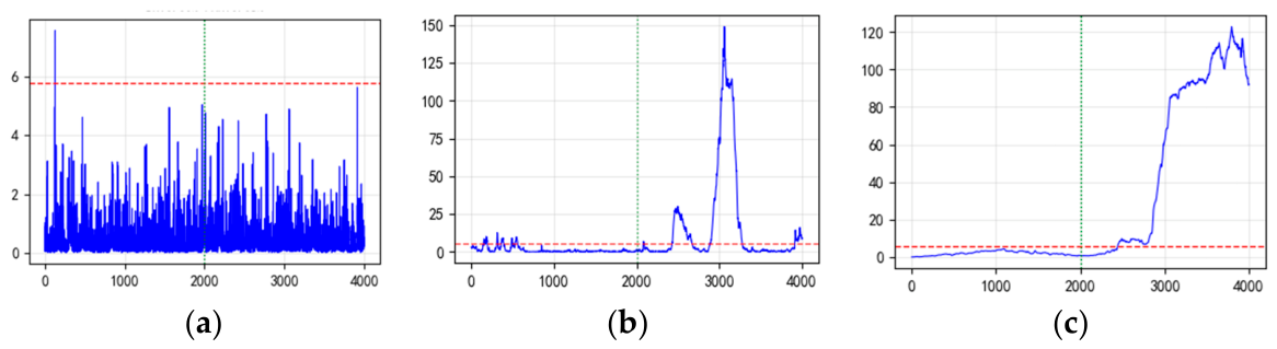
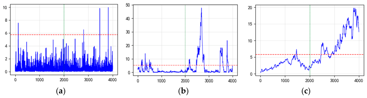
For detailed illustration, the detection trajectories obtained by the three methods are compared in Figure 3 and Figure 4, where the red dashed line denotes the control limit and the green dotted line marks the time instant at which the fault is introduced.

4.2. CWRU Bearing Dataset

The CWRU bearing dataset serves as an internationally recognized benchmark for validating bearing fault diagnosis algorithms. In this study, vibration signals were acquired at a sampling frequency of 48 kHz from the experimental platform, which consists of a motor, a torque transducer, and related data acquisition equipment. The dataset includes artificially introduced single-point faults on the inner race, outer race (at 3, 6, and 12 o’clock positions), and rolling elements, generated via electrical discharge machining to simulate realistic localized damage. A total of 13 distinct fault conditions are systematically categorized based on fault location and size, providing a comprehensive foundation for evaluating diagnostic model performance under varying fault types and severity levels.

The performance of the proposed method on the CWRU dataset is comprehensively summarized in

Table 3. FDRs (%) for different fault types in the CWRU bearing dataset.

Index	Fault Location	Fault Size	DiPCA	ARMA	The Proposed Method
1	Ball	7	21.05	99.30	96.45
2		14	16.35	66.20	92.75
3		21	28.30	96.35	91.65
4	Inner race	7	69.55	98.50	97.85
5		14	28.90	55.85	74.20
6		21	79.25	96.80	98.35
7	Outer race at 3 o’clock positions	7	82.40	99.40	98.80
8		21	89.35	100.00	100.00
9	Outer race at 6 o’clock positions	7	93.15	99.65	98.95
10		14	17.30	92.60	96.85
11		21	67.85	86.75	92.20
12	Outer race at 12 o’clock positions	7	37.85	99.25	98.40
13		21	39.65	86.30	95.20
Average FDR	/	/	51.61	90.53	94.74

. To ensure a fair comparison, all deep models were configured with consistent hyperparameters: a fixed random seed of 42, a sliding-window size of 1000, the Adam optimizer with a learning rate of 0.001, and 100 training epochs. For the proposed method, the top 5 singular values were retained, the lag order was s = 2, the number of latent variables was l = 5 for DiPCA, and the ARMA-Transformer used a hidden dimension of 64 with four attention heads. Control limits were computed via KDE at a confidence level of 99% (α = 0.01). The comparative results further highlight the advantage of the integrated framework over the individual DiPCA and ARMA baselines. For the ball fault with a fault size of 14 mils, DiPCA achieves an FDR of only 16.35% and ARMA achieves 66.20%, whereas the proposed method significantly improves the detection rate to 92.75%. For the inner race fault with a fault size of 14 mils, DiPCA achieves only 28.90% and ARMA achieves 55.85%, while the proposed method attains 74.20%. For the outer race fault at the 12 o’clock position with a fault size of 21 mils, DiPCA achieves only 39.65% and ARMA achieves 86.30%, compared to 95.20% achieved by the proposed method. In terms of average FDR, the proposed method achieves 94.74%, substantially outperforming DiPCA (51.61%) and ARMA (90.53%). These results collectively demonstrate the superiority and generalization capability of the proposed integrated monitoring framework in bearing fault detection tasks.

5. Discussion

Because no physical model is required, data-driven fault detection is a widely studied research topic in dynamic processes. The experimental findings presented in this study demonstrate the efficacy of the ARMA-Transformer DiPCA framework for incipient fault detection in complex industrial systems. The superior performance observed across both the TEP and the CWRU bearing datasets can be attributed to several methodological innovations inherent in the proposed approach.

Primarily, the integration of a masked linear ARMA attention mechanism within the Transformer architecture addresses a fundamental limitation of conventional process monitoring techniques. Traditional statistical methodologies, including PCA and DPCA, are predicated on linear assumptions. Consequently, they cannot adequately capture the complex temporal dependencies of industrial processes. By incorporating ARMA dynamics into the attention mechanism, the proposed method effectively models both autoregressive patterns and MA components. This enables a more precise characterization of process dynamics and fault signatures.

Furthermore, the synergistic combination of deep learning components with the established DiPCA statistical framework constitutes a robust monitoring system. While deep learning models exhibit superior capability in capturing complex nonlinear relationships, they often lack the statistical rigor required for reliable process monitoring. Here, the DiPCA foundation provides a statistical framework for residual analysis and control limit determination, ensuring that the proposed method maintains a low average FAR of 0.067% across all TEP fault scenarios while simultaneously achieving enhanced detection sensitivity. This low false alarm rate, together with the interpretable control limits derived from the statistical framework, helps reduce operator burden in practical applications.

To assess the practical deployability of the proposed method, its computational complexity and real-time performance are examined. All experiments were conducted on a computer equipped with an Intel Core Ultra 9 285H CPU and 16 GB of RAM, using Python 3.13 and PyTorch 2.8.0 (CPU-only). Across the 22 TEP fault scenarios, the average training time was 5.3 s, and the average test time was 3.4 s. The test time corresponds to processing 4000 samples, yielding an average inference latency of approximately 0.85 ms per sample. This per-sample latency is well within the sampling interval of three minutes in the TEP benchmark, confirming that the proposed method is suitable for real-time industrial process monitoring. Notably, these results were achieved without GPU acceleration, indicating that the method can be deployed on modest industrial computing hardware. The short training time further suggests that the model can be periodically retrained or updated without disrupting online operations.

The observed performance variations across different fault categories merit further investigation. For TEP faults 3 and 9, the proposed method demonstrates substantial improvements over conventional approaches, suggesting that the ARMA-Transformer component is particularly effective at detecting faults characterized by subtle, slowly evolving deviations. The comparatively lower performance on fault 5 relative to faults 3 and 9 may be attributed to the specific dynamic characteristics associated with condenser cooling-water temperature perturbations, which may present greater detection challenges. For fault 5, the step change introduces only a subtle shift in a single variable. Since the sliding-window SVD captures the dominant energy structure of the windowed data, this low-amplitude perturbation is easily diluted by other high-energy variables, resulting in singular value features that carry insufficient fault information for the downstream DiPCA and ARMA-Transformer stages. For fault 15, which also exhibits modest detection rates, the valve sticking fault produces intermittent transient deviations that occur only when the valve is commanded to move. The fixed-weight AR attention captures stable temporal patterns, and the MA component further smooths short-term residual fluctuations through its exponential decay structure. As a result, the transient signatures may be partially attenuated before reaching the monitoring statistics, leading to discontinuous threshold exceedances and a lower overall FDR. These cases indicate that while the deep integration of the ARMA-Transformer with DiPCA enhances sensitivity to slowly evolving incipient faults, the reliance on singular value features and the smoothing effect of the MA decay structure can reduce responsiveness to isolated transient events and single-variable perturbations.

For the CWRU dataset, the consistently high performance across the majority of fault conditions substantiates the method’s generalization capability to mechanical systems. The exception of condition 5 (74.20% FDR) indicates that certain fault orientations may pose specific challenges for vibration-based detection methodologies. This phenomenon could be attributable to the directional sensitivity of vibration sensors or to distinct propagation patterns associated with faults at the inner race with a 14-size defect. At this intermediate defect size (14 mils), the fault-induced impulses are weaker than those of larger defects (21 mils), while the increased randomness from the larger damaged area makes the fault signature less periodic than that of smaller defects (7 mils). The sliding-window SVD extracts dominant singular value patterns and may not fully preserve these weak and partially irregular impulses. The fixed-weight AR attention captures stable latent dynamics, and the MA component applies temporal smoothing to the residuals. For vibration signals with irregular transient impulses, this smoothing can attenuate fault signatures before they reach the monitoring statistics. Despite these effects, the FDR of 74.20% remains substantially higher than the DiPCA-only result of 28.90% and the ARMA-only result of 55.85%, indicating that the integrated framework retains considerable fault sensitivity even under suboptimal conditions.

The practical implications of these findings hold significant relevance for industrial applications. The ability of the proposed method to maintain low FARs while achieving high detection sensitivity addresses a critical operational requirement in process industries. False alarms and undetected faults can lead to unnecessary production interruptions and economic losses. Moreover, the method’s efficacy in detecting small-scale faults underscores its potential for predictive maintenance applications, facilitating early intervention prior to the escalation of faults into catastrophic failures.

6. Conclusions

This research addresses the core challenge of detecting incipient faults in complex industrial processes. It proposes an enhanced DiPCA based on ARMA-Transformer. The method combines the ARMA structure for modeling temporal patterns with the Transformer architecture for capturing long-range dependencies. To overcome this limitation, a masked linear ARMA attention mechanism is introduced to replace the linear dynamic component of DiPCA. Tests on the TEP show that this method detects typical incipient faults 3 and 9 at much higher rates than conventional methods. In addition, tests on the CWRU bearing dataset confirm that the method works well for mechanical systems. The main contribution of this work is an embedded architecture that integrates deep learning with traditional statistical process monitoring. The neural network is placed inside DiPCA as its dynamic engine rather than added as an external module, offering an effective solution for industrial process safety monitoring. However, the effectiveness of the proposed method under time-varying process dynamics and real industrial conditions remains to be further investigated, as current validation primarily focuses on standard benchmarks. Future work will include validation on real minute-level industrial datasets from large-scale chemical enterprises to assess the method’s performance under actual sensor noise, variable coupling, and temporal irregularities.