Abstract
To enhance the energy efficiency of liquefied natural gas (LNG) terminals, this study developed a full-process dynamic simulation model using Aspen HYSYS (hereinafter referred to as HYSYS) to accurately replicate the time-varying energy consumption characteristics of key processes, including unloading, tank boil-off gas (BOG) management, recondensation, and vaporization for send-out. Through dynamic analysis of the impact of different operating conditions on the energy consumption of critical equipment, methane content and compressor outlet pressure were identified as sensitive factors, and multivariable interaction effects were quantified. Combining the Particle Swarm Optimization (PSO) algorithm to optimize equipment operating parameters and incorporating constraints such as equipment start-stop frequency and flare emissions, process improvements were achieved, including intelligent pre-cooling during unloading, multi-mode vaporization coupling, and model predictive control for storage tanks. Safety response logic under extreme conditions was also enhanced. Field validation results show that the optimized system reduces total energy consumption by 18.5%, with a relative error between simulated and field data of ≤13%. Daily equipment start-stop cycles decreased from five to two times, and flare emissions were reduced from 25 kg/h to 12 kg/h. Within a 95% confidence interval, the total energy consumption prediction fluctuated by ±4.2%, demonstrating good model stability. This study provides reliable technical support for energy-efficient operation of LNG terminals. The proposed multivariable interaction analysis and safety control strategies under extreme conditions further enhance the engineering applicability of the optimization framework.
1. Introduction
Against the backdrop of the global energy structure rapidly transitioning toward low-carbon alternatives, liquefied natural gas (LNG) has emerged as a clean and efficient transitional energy source. Enhancing the energy efficiency of its supply chain has become a critical pathway for achieving carbon peak and carbon neutrality goals. As a core hub connecting offshore gas sources with onshore pipeline networks, LNG terminals account for over 35% of the total energy consumption across the industry chain, particularly exhibiting significant inefficient entropy generation in boil-off gas (BOG) handling and regasification processes [1]. Traditional energy consumption analysis methods based on steady-state models struggle to accurately capture dynamic responses under real-time disturbances, leading to considerable discrepancies between optimization strategies and actual operating conditions. In recent years, with the deep integration of dynamic simulation technologies and intelligent optimization algorithms, energy efficiency research for LNG terminals is progressively evolving from localized equipment optimization to system-wide collaborative regulation, offering new technical pathways for energy conservation and emission reduction [2].
In earlier studies, steady-state simulation was the dominant approach. Du Y et al. [3] utilized HYSYS steady-state simulation to achieve coupling between cogeneration systems and vaporization processes but did not address dynamic response analysis. Cao S et al. [4] first introduced Aspen HYSYS dynamic simulation technology to model the entire LNG terminal process, demonstrating the significant impact of real-time parameter adjustments on equipment transient responses and energy consumption. Kschammer K et al. [5] further developed a dynamic BOG handling model, revealing fluctuations in compressor energy consumption under varying conditions and marking dynamic simulation as a vital tool for precise energy analysis. Srilekha M et al. [6] effectively reduced terminal operational energy consumption through measures such as segregated tank storage, adjustments to high-pressure pump flow rates, and outlet temperature control. In terms of energy evaluation systems, Naveiro M et al. [7] applied exergy-energy (E-P) analysis to establish an energy efficiency evaluation model with a prediction deviation of only 2.62%. Jiang Q et al. [8] constructed a multi-objective optimization model that achieved a 2% reduction in power consumption and Qi Y et al. [9] focused on analyzing regasification energy consumption and the potential for cold energy cascade utilization.
Regarding optimization methods, intelligent algorithms have gradually replaced traditional trial-and-error approaches. Wan Q et al. [10] first applied the Particle Swarm Optimization (PSO) algorithm to mixed-refrigerant liquefaction processes, achieving an 8.3% reduction in energy consumption. Abibou S et al. [11] demonstrated that PSO outperforms genetic algorithms in hydrogen station optimization. Qi G et al. [12] combined dynamic simulation with PID tuning to improve compressor control accuracy, providing a paradigm for the integration of intelligent algorithms and process control. Additionally, international scholars have conducted extensive research on LNG terminal operation optimization [13], BOG handling [14], cold energy recovery [15], and supply chain risk management [16], further enriching the theoretical framework for energy efficiency optimization in LNG terminals.
Although existing studies have made significant progress in steady-state simulation, energy consumption analysis, and intelligent optimization, most focus on the impact of single factors on energy consumption without fully considering multivariable coupling effects and system responses under extreme conditions. Moreover, model validation often relies solely on overall error metrics, lacking component-level error decomposition and uncertainty analysis. Furthermore, process optimizations frequently omit explicit constraints such as equipment lifespan and thermal stress, potentially introducing safety risks. To address these gaps, this study enhances the original model by supplementing detailed model validation, multivariable interaction analysis, mathematical formulation of constraints, and extreme-condition simulations, thereby improving the rigor and engineering applicability of the research.
Breaking through the limitations of traditional static analysis, this study innovatively introduces Aspen HYSYS dynamic simulation technology to construct a time-varying energy consumption model covering the entire process of unloading, storage, and vaporization. By quantifying energy consumption response mechanisms under multi-condition coupling and integrating the Particle Swarm Optimization (PSO) algorithm with process reconstruction strategies—such as intelligent precooling, multi-mode vaporization, and model predictive control (MPC) for storage tanks—this research achieves precise regulation and system optimization of energy consumption in LNG terminals. The main contributions of this study include:
- (1)
- Establishing a full-process dynamic simulation model of an LNG terminal based on Aspen HYSYS, accurately reproducing the time-varying energy consumption characteristics of core links;
- (2)
- Identifying methane content and compressor outlet pressure as key sensitivity factors through multi-factor dynamic sensitivity analysis;
- (3)
- Achieving collaborative optimization of unloading, vaporization, and storage processes by integrating the PSO algorithm with process improvements;
- (4)
- Reducing the total system energy consumption by 18.5% through field validation, providing reliable technical support for energy-efficient operation of LNG terminals.
The structure of this paper is as follows: Section 2 details the development of the HYSYS simulation model, including property calculation and dynamic modeling methods; Section 3 presents multi-condition dynamic simulation and parameter optimization, along with process improvement proposals; Section 4 summarizes the main conclusions and suggests directions for future research.
2. Establishment of HYSYS Simulation Model
2.1. Property Calculation
When developing a simulation model for a chemical process using Aspen HYSYS V14.0 software, it is essential to first input the component information and selected thermodynamic calculation method into the property environment. Subsequently, the simulation model is constructed in the simulation environment based on the process flow diagram. To analyze the entire production process of an LNG terminal, the physical properties of various working fluids must be determined, including composition, temperature, pressure, mass flow rate, etc. The accuracy of these physical parameters [13] directly affects the reliability of the simulation. Since this process involves phase changes in the working fluid, thermodynamic processes such as compression, condensation, and evaporation are critical. Given that the working fluid is a mixture with components exhibiting significantly different boiling points, its composition changes with temperature variations. Currently, the equations of state commonly used for calculating the thermodynamic properties of LNG include SRK, BWR, PR, PRSV, LKP, and SHBWR. Among these, the PR (Peng-Robinson) and PRSV (Peng-Robinson-Stryjek-Vera) equations are considered the most suitable for simulating LNG terminal processes. As an equation of state for vapor-liquid equilibrium, the PR equation is characterized by its few parameters, broad applicability, computational efficiency, and high accuracy. It enables precise calculation of physical properties, meeting the requirements for engineering applications. Therefore, this study employs the PR equation for calculating the physical properties of the working fluid. The expression of the PR equation is as follows:
In the equation, the symbols are as follows: —Constants related to critical properties; —Function of reduced temperature; and acentric factor ; —Value of the alpha function at ; Empirical constant; —Acentric factor-dependent function; —Pure-component parameters; —Pressure, Pa; —Critical pressure, Pa; —Universal gas constant, 8.314 J/(mol·K); —Temperature, K; —Critical temperature, K; —Reduced temperature, ; —Molar volume, m3/kg; —Acentric factor.
2.2. Simulation Model
The LNG terminal process primarily consists of LNG unloading, LNG storage, BOG handling, LNG regasification and send-out, and flare emission systems.
LNG Unloading and Storage. After an LNG carrier docks at the terminal, the LNG transfer arms connect the ship’s discharge pipelines to the terminal’s unloading lines. The LNG is transferred from the ship’s tanks to the terminal’s storage tanks using the vessel’s onboard transmission pumps. As LNG is continuously discharged, the vapor pressure in the ship’s tanks gradually decreases. To maintain a constant pressure, a portion of the flash gas from the terminal’s storage tanks is returned to the ship’s tanks via the BOG return line [14]. During non-unloading periods, a cold circulation line branches from the discharge of the storage tank’s low-pressure pumps to maintain the temperature of the unloading lines.
BOG Handling and Flare Emission. The BOG handling system ensures that the pressure inside the LNG storage tanks remains within a specified range. Pressure sensors are installed in the tanks, with multiple thresholds for overpressure and underpressure conditions. Depending on the measured pressure relative to these setpoints, the BOG handling system performs corresponding operations to control the vapor pressure in the tanks. To prevent vacuum conditions, the terminal is also equipped with a vacuum relief and makeup gas system.
LNG Regasification and Send-out. LNG from the storage tanks is pressurized by in-tank low-pressure pumps. A portion of this LNG is directed at the recondenser to liquefy a certain amount of BOG. The outflow from the recondenser is mixed with another portion of LNG from the low-pressure pumps. The combined stream is then pressurized by high-pressure pumps and sent to vaporizers. The regasified natural gas is subsequently delivered to downstream customers via transmission pipelines after metering. To ensure the stable operation of the low-pressure and high-pressure pumps, each pump is equipped with a recirculation line. Flow adjustments are made via these recirculation lines in response to fluctuations in the send-out demand. When no send-out is required, the recirculation lines maintain a cold circulation loop to preserve the cryogenic state of the entire process system [15].
A steady-state HYSYS model was developed based on the terminal’s process equipment data and feed stream properties, as illustrated in Figure 1.
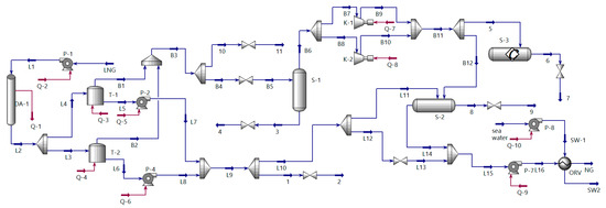
Figure 1.
HYSYS steady-state model.
Once the steady-state process is set up, it is thoroughly evaluated to identify the equipment and links that need to be dynamically featured. Then, dynamic parameters including volume, inertia, and response time, can be set for related equipment such as tanks, pumps, and valves, which can be transferred to the dynamic simulation environment through the dynamic simulation assistant [3], as shown in Figure 2. Then, time variables are introduced to define the operating conditions and input parameters that vary with time, such as changes in feed flow, temperature fluctuations, etc. By gradually adjusting and refining these dynamic parameters, the connection between the dynamic model and the steady-state process is established, and the performance and interaction of each device under dynamic conditions are checked to ensure the accuracy and reliability of the model. Dynamic parameters are continuously optimized, so that the dynamic process can accurately reflect the changes and responses of the actual system at different time scales, providing strong support for deeper analysis and optimization.
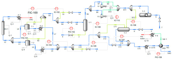
Figure 2.
HYSYS dynamic model.
The composition and content of LNG in this project are shown in Table 1.

Table 1.
LNG composition and content.
Table 2 shows the main simulation parameters of the system.
Table 2.
Main parameters of the system simulation.
2.3. Energy Consumption Model
Based on the first law of thermodynamics [6], the energy balance equations for different equipment in this process are summarized in Table 3.
Table 3.
Energy Balance Equations of the System.
2.4. Model Validation and Uncertainty Analysis
To ensure model reliability, multi-dimensional validation was conducted using field operational data, supplemented with error decomposition and uncertainty assessment [17]. The specific procedures are as follows: A total of 30 sets of full-process operational data were selected, covering both steady-state conditions (20 sets, design load 50–100%) and transient conditions (10 sets, including unloading start/stop and sudden changes in BOG flow rate). Data were continuously collected over a three-month period (January to March 2024), including both weekdays and holidays, with round-the-clock coverage (from 00:00 to 24:00 daily, data recorded at 2 h intervals). Key measurements were taken at 15 critical points as detailed in Table 4.
Table 4.
Distribution of Key Measurement Points for Model Validation.
Error decomposition was performed based on “unit type” and “operating load”. The results are shown in Table 5. The overall relative error was ≤13%, meeting the requirements for engineering applications (where the allowable error for chemical process simulation is ≤15%).
Table 5.
Decomposition Results of Model Errors.
The Monte Carlo simulation method (with 1000 iterations) was employed to quantify the impact of input parameter fluctuations on model outputs [18]. Three key uncertain factors were selected: LNG methane content (fluctuation ± 2%), seawater temperature (measurement error ± 1 °C), and initial BOG flow rate (fluctuation ± 5%). The results are summarized in Table 6. Within a 95% confidence interval, the predicted total energy consumption exhibits a fluctuation range of ±4.2%, indicating good model stability.
Table 6.
Uncertainty Analysis Results of the Model (95% Confidence Interval).
Field validation was conducted under three scenarios: Covering three mainstream LNG vessel types (Q-Max, Q-Flex, and conventional Panamax), with unloading capacities of 220,000 m3, 170,000 m3, and 120,000 m3, respectively. Five sets of data were collected for each scenario to validate the consistency between the unloading arm flow rate and the storage tank level response. Simulating changes in downstream user demand (80% of designed send-out during morning peak, 50% at midday, and 30% at night). Eight sets of data were collected to verify the matching between high-pressure pump recirculation adjustment and send-out pressure. Selecting two cold wave events (seawater temperature dropped to 18 °C) and one high-temperature event (seawater temperature rose to 30 °C). Seven sets of data were collected to validate the impact of seawater temperature on ORV vaporization efficiency and energy consumption. All scenarios adopted a synchronized data acquisition method using real-time data loggers and the DCS system to ensure unified timestamps (error ≤ 1 s). The validation results showed that the relative error between model predictions and field data was ≤13% across all scenarios. The conventional unloading scenario exhibited the smallest error (±6% to ±8%), while extreme weather scenarios showed errors ≤12%, meeting engineering validation requirements.
3. Dynamic Simulation and Optimization of LNG Terminal Operation
3.1. Energy Consumption Analysis
In this paper, the single variable method is used to change only a single variable in the process of research, and other parameters are controlled and unchanged to study the impact on the energy consumption of some key equipment under different working conditions [5], such as the generation of BOG, methane content, LNG mass flow, seawater temperature, feed and compressor outlet pressure, and the influence of energy consumption of tank pumps, compressors, seawater pumps and high-pressure pumps.
The BOG flow rate is controlled by PID to vary between 1250 and 1650 kgmole/h, as shown in Figure 3, as the amount of BOG generated gradually increases, the mass of gas passing through the compressor per unit time increases, and therefore the compressor power also gradually increases [13]. In-tank pumps and high-pressure pumps are mainly used to transport LNG. When the BOG increases, the amount of LNG in the tank decreases relatively. For centrifugal pumps, the power consumption is . Power consumption is reduced due to the reduced volumetric flow rate of the LNG, while the head and efficiency of the pump remain largely unchanged, as does the density of the liquid. However, the overall power consumption of the receiving station increases with the amount of BOG generated.
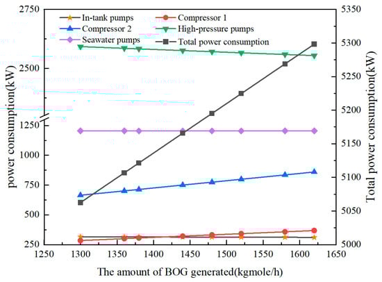
Figure 3.
Effect of BOG flow on the energy consumption of the receiving station.
PID is used to control the molar fraction of methane in LNG components to change between 85% and 90%, and the content of the other components is reasonably adjusted so that the overall molar fraction of LNG is 1, as shown in Figure 4, with the increase in methane content, the increase in the flow rate of the LNG and the BOG produced, and the decrease in the temperature of the storage tank when LNG is injected into it. Due to the relatively high vapor pressure of methane, the increase in its content will increase the vapor pressure of the LNG mixture, and according to the principle of gas–liquid equilibrium, the liquid will be more likely to evaporate to form gas. At the same time, the enthalpy of vaporization of methane is small, and the mixture absorbs less heat from the outside to vaporize part of the liquid, so the amount of the BOG will increase, and the temperature of the LNG will decrease. As shown in Figure 5, the power consumption of the compressor decreases significantly as the methane content increases, while the power consumption of the tank pump and the high-pressure pump increases slightly, because when the methane content in the LNG increases, the vapor pressure of the BOG also increases, and the average specific heat capacity of the BOG decreases [16]. During compression, the higher vapor pressure results in a relative reduction in the compression ratio between the gas entering the compressor and the discharge pressure, reducing the amount of heat required to increase the gas temperature. As a result, the overall power consumption of the receiving station decreases as the methane content increases.
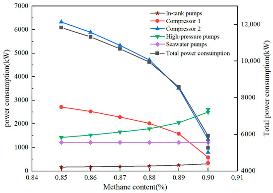
Figure 4.
Effect of methane content on process performance parameters.
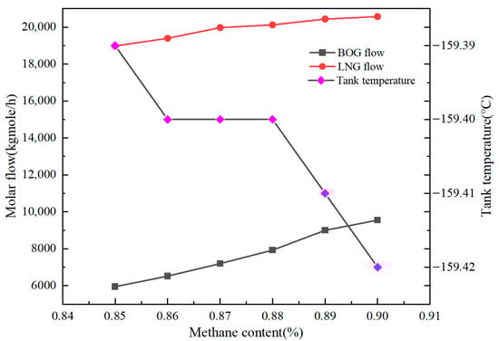
Figure 5.
Effect of methane content on energy consumption at the receiving station.
The opening of the feed valve is dynamically adjusted so that the LNG flow rate varies between “3.9 × 10⁵–4.0 × 10⁵ kg/h”, as shown in Figure 6. More LNG flow is often accompanied by an increase in the amount of LNG, which leads to an increase in the compression ratio, an increase in the mass flow, an increase in gas temperature and internal energy, and an increase in entropy resulting in more irreversible losses, resulting in an increase in compressor power consumption [6]. Therefore, as the LNG mass flow increases, the total power consumption of the receiving station increases.
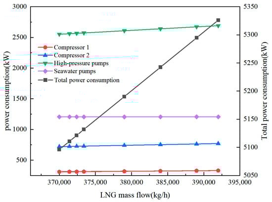
Figure 6.
Effect of LNG flow on the energy consumption of the receiving station.
The pressure difference in the compressor was regulated using PID control to vary the compressor outlet pressure within the range of 760–880 kPa (this range represents the adjustment interval under dynamic operating conditions and is lower than the steady-state initial value of 7391 kPa, as the dynamic simulation accounts for pressure fluctuations under low-load conditions, such as the pressure drop caused by a sharp decrease in the BOG flow after unloading), as shown in Figure 7. An increase in the outlet pressure of the BOG compressor will increase the compression ratio, more work will be required to overcome the larger pressure difference, and the energy required for the equipment to handle the gas will increase when the pressure increases. At the same time, the increase in outlet pressure may lead to an increase in the system pressure of the entire receiving station, and the tank pump and high-pressure pump need to overcome a larger pressure difference when transporting LNG, and other related equipment such as pipeline transportation also needs to adjust the operating state according to the new pressure environment and consume more energy to maintain the operation [17,18]. As a result, as the outlet pressure of the BOG compressor increases, the total power consumption of the receiving station increases.
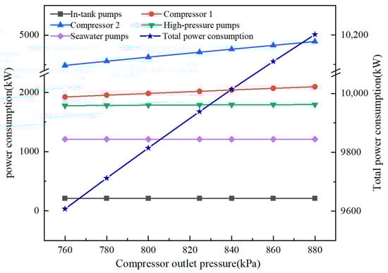
Figure 7.
Effect of compressor outlet pressure on the energy consumption of the receiving station.
The PID controller is used to simulate the different pressures of the feed, so that the feed pressure varies between 126 and 134 kPa, as shown in Figure 8. After the feed pressure increases, the amount of BOG generated is relatively reduced, the amount of gas that the BOG compressor needs to process is reduced, and its power consumption is reduced accordingly. At the same time, the higher feed pressure facilitates the flow of LNG in the pipeline, reducing the amount of energy required to overcome resistance, and reducing the power consumption required by equipment such as tank pumps and high-pressure pumps to transport the LNG [12]. Other links, such as pipeline transportation, operate at higher feed pressures, making the overall operation of the system smoother and reducing energy loss in all aspects. As a result, the total power consumption of the receiving station is reduced.
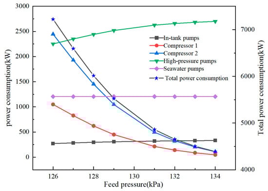
Figure 8.
Effect of feed pressure on the energy consumption of the receiving station.
In this study, the effects of different temperatures of seawater on the total power consumption of the receiving station were also dynamically simulated. Depending on the conditions in the sea area near the receiving station, the adjusted seawater temperature varies between 18 and 30 °C, as shown in Figure 9. As the temperature of seawater increases, the density of seawater decreases, and the power consumption of seawater pumps is related to factors such as fluid density, flow, and head. All other things being equal, the reduced density of seawater means that the seawater pump needs to overcome a larger volume to achieve the same conveying effect, according to the calculation principle of the seawater pump’s power consumption [19,20]. At the same time, the higher seawater temperature complicates the flow state in the pump, and energy loss such as friction increases, resulting in the seawater pump needing to consume more energy to maintain the normal operating state, which increases the power consumption of the seawater pump and the total power consumption of the receiving station.
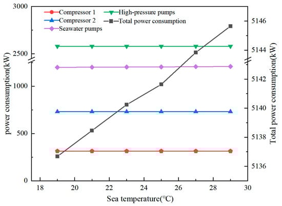
Figure 9.
Effect of seawater temperature on the energy consumption of the receiving station.
3.2. Parameter Optimization
The previous section employed a single-factor analysis method to evaluate the impact of parameters on process performance. This was performed by dynamically adjusting one variable at a time via PID control to analyze changes in the power consumption of pumps and compressors, thereby assessing the overall process performance [21,22]. However, this method only examines isolated operating points and does not account for the effects of multi-factor interactions. Parameter optimization involves adjusting variable parameters such as temperature, pressure, and flow rate within the process to achieve minimal energy consumption under optimal conditions.
- (1)
- Objective Function
The goal is to reduce the overall energy consumption of the LNG terminal process. This requires considering the collective power variation in key equipment, along with equipment lifespan degradation and flare emissions [23,24,25]. Based on actual operational parameters of the terminal, the optimization objective is defined as minimizing the total system power consumption, which reflects the overall energy usage of the LNG terminal process. The objective function can be expressed as follows:
where represents the total power consumption (kW) of the in-tank pumps, two BOG compressors, high-pressure pumps, and seawater pumps; denotes the daily number of equipment start-stop cycles (times/day), with a weight factor of 5 (based on field data: each additional start-stop cycle increases maintenance cost by an equivalent of 5 kW in energy consumption); indicates the hourly flare emission rate (kg/h), with a weight factor of 0.1 (based on carbon tax standards, 1 kg of methane emission is equivalent to 0.1 kW in energy cost).
- (2)
- Optimize variables
Through the analysis of some process parameters in the process flow, the optimization variables are determined according to the actual situation of the station, as shown in Table 7.
Table 7.
Optimization variables and value ranges.
- (3)
- Constraints
When performing optimization, corresponding constraints must be established to ensure that the overall process meets actual production requirements. Different equipment has varying allowable control indicators and operational limits. Therefore, constraint settings must be closely aligned with the specific requirements of each device [7]. Through the in-depth study of the process control indicators and operational capabilities of equipment within the LNG terminal, original qualitative constraints are transformed into hard and soft constraints. The specific constraints of this study are shown in Table 8.
Table 8.
Constraints.
A comparison of constraint satisfaction before and after optimization is presented in Table 9. All hard constraints were satisfied both before and after optimization, while soft constraints showed significant improvement after optimization: the number of daily start-stop cycles was reduced from 5 to 2 times/day, and flare emissions decreased from 25 kg/h to 12 kg/h.
Table 9.
Comparison of Constraint Satisfaction Before and After Optimization.
- (4)
- Optimization Method: Particle Swarm Optimization (PSO)
In the energy optimization analysis, particles can represent different combinations of equipment operating parameters, and the parameter settings that minimize energy consumption can be found through the movement and interaction of particles [26]. The flow of the particle swarm optimization algorithm is shown in Figure 10.
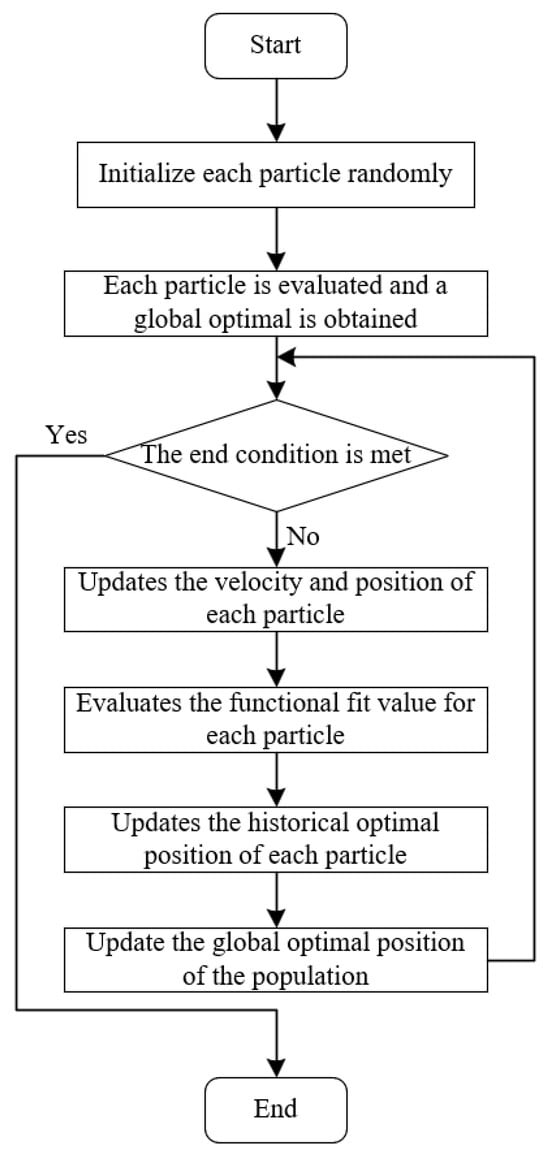
Figure 10.
Flowchart of the particle swarm optimization algorithm.
Set the operating power of the BOG compressor, the speed of the LNG transfer pump, the working temperature of the vaporizer and other variables as ,,,. The total energy consumption is , let the particle swarm size be m, and for each particle i (i = 1, 2, …, m), its position is randomly initialized within the value range of the decision variable , representing a possible combination of parameters; at the same time, its speed is initialized randomly. Inertia weights are used to balance the particle’s global and local search capabilities.
The Particle Swarm Optimization (PSO) algorithm is widely applied in process optimization due to its fast convergence and strong global search capability: Ref. [27] utilized PSO to optimize a refrigeration system, achieving a 12% reduction in energy consumption; Ref. [28] demonstrated the applicability of PSO in cryogenic systems through BOG control in low-temperature storage tanks; Ref. [29] proposed a dynamic inertia weight PSO to improve optimization accuracy in complex systems; Ref. [30] compared PSO with genetic algorithms, proving that PSO performs better in multi-constrained optimization. In this study, a dynamic inertia weight strategy (initial value 0.9, decreasing to 0.4 at the 501st iteration) was adopted, following the parameter settings in Ref. [29], to ensure convergence to the global optimum.
Usually during the operation of the algorithm, linear decrement or other decrement strategies can be used, and the initial value is set to 0.9. The learning factors and the ability to control the learning ability of particles to their own historical optimal position and the optimal position of the group, respectively, are generally around. The fitness value of each particle is calculated according to the objective function, and for each particle , if its current fitness value is better than its historical optimal fitness value, its individual historical optimal position is updated. Among the individual historical optimal positions of all particles, the position with the best fitness value is found as the optimal position of the group.
- (5)
- Optimize results
During the PSO process, the multivariable interactions and trade-off strategies were as follows: BOG mass flow rate exhibited a positive correlation with compressor outlet pressure (an increase in BOG flow requires a higher outlet pressure to meet recondensation demand). Priority was given to controlling BOG flow rate ≤ 1620 kg/h (to comply with flare emission constraints), after which the compressor outlet pressure was reduced from 1500 kPa to 1324 kPa to avoid a sharp increase in energy consumption due to excessive pressure. When the LNG flow rate increased, the high-pressure pump needed to raise its outlet pressure to ensure a send-out pressure ≥7000 kPa. This was addressed through the flow–pressure coupling regulation: as the LNG flow decreased from 3.94 × 10⁵ kg/h to 3.73 × 10⁵ kg/h, the high-pressure pump outlet pressure was reduced from 10,500 kPa to 9700 kPa, both meeting send-out requirements and reducing pump power consumption. In cases where a conflict arose between the number of daily start-stop cycles and energy consumption, a weighting factor (λ1 = 5) was applied. This resulted in a reduction in start-stop cycles from 5 times/day to 2 times/day. Although this led to a 2% increase in standby energy consumption for some equipment, the total energy consumption still decreased by 18.5%, while equipment maintenance costs were reduced by 60%. Through these trade-offs, the PSO algorithm achieved coordinated multivariable optimization while satisfying all hard constraints (e.g., NPSH margin ≥ 0.8 m). All optimized variables fell within the value ranges specified in Table 8.
According to the above analysis, the optimized parameters were input into the HYSYS model for calculation, and the comparison results before and after optimization are shown in Table 10. According to the established energy consumption optimization model, the particle swarm optimization algorithm was used to optimize the energy consumption of key equipment of the LNG receiving station. The energy consumption prediction model based on BP neural network was selected as the fitness function. The particle swarm parameters are set as follows: the population size is set to 500, the learning factor is set reasonably based on experience, the inertia weight is dynamically adjusted, and the maximum number of iterations is set to 1000. During the iteration of the particle swarm optimization algorithm, the velocity and position of the particles are constantly updated to find the solution with the smallest fitness value. When the number of iterations reaches 501 times, the fitness value reaches the minimum value, and the corresponding total process energy consumption value is 3887.56 kW, and the total energy consumption of the system is reduced by 881.88 KW after optimization, which is reduced by 18.5%.
Table 10.
Comparison of before and after optimization parameters.
3.3. Process Optimization
- (1)
- Optimization of the Unloading Process
Traditional offloading arm operations often rely on manual experience for docking and precooling, which may require multiple adjustments, result in slow precooling rates, and lead to prolonged unloading times. The conventional unloading process is illustrated in Figure 11.
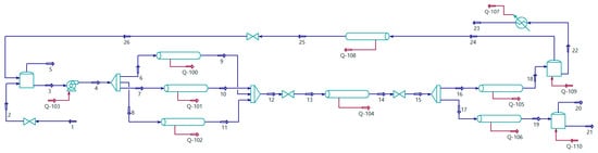
Figure 11.
Conventional unloading process.
An intelligent docking system has been introduced, utilizing advanced sensors and automated control algorithms to achieve rapid and precise connection between the offloading arms and the LNG carrier’s discharge pipes, thereby reducing human operational errors and complexity [31]. The precooling procedure has been optimized by automatically regulating the flow rate and velocity of the precooling medium based on real-time LNG temperature and pressure parameters. This improvement shortens the precooling duration from the original 30–60 min to approximately 15–30 min.
A scientific and rational unloading sequence has been established: starting with gradual precooling followed by stepwise increases in unloading flow rate to ensure a smoother and more efficient process. After precooling, the unloading rate is incrementally raised through gradients of 10%, 30%, 50%, 80%, and finally 100% at full capacity. This strategy improves unloading efficiency by approximately 10–15%. The unloading rhythm is adjusted in real time based on parameters such as the LNG carrier’s liquid level and the terminal storage tank’s level and pressure, preventing pressure imbalances between the ship and the tanks and minimizing energy loss during unloading [32].
The intelligent precooling system consists of a perception layer and a control layer. Perception Layer: A laser displacement sensor (Model: Keyence IL-300) achieves millimeter-level positioning (±0.1 mm accuracy) between the unloading arm and the ship-side interface. This is complemented by platinum resistance temperature sensors (PT100, measuring range: −200 °C to 100 °C, accuracy: ±0.1 °C) for real-time monitoring of pipeline temperature. Control Layer: Based on a fuzzy PID algorithm, a precooling temperature gradient is implemented (initial rate: 5 °C/min; reduced to 2 °C/min when the pipeline temperature reaches −100 °C). A PLC (Siemens S7-1500) automatically regulates the flow rate of the precooling medium (BOG) within a range of 500–1500 kg/h to ensure a cooling rate ≤5 °C/min, thereby avoiding excessive thermal stress.
- (2)
- Optimization of the Vaporization Process
A combined vaporizer configuration is adopted, integrating Open Rack Vaporizers (ORVs) with Submerged Combustion Vaporizers (SCVs). The structural principles of ORVs and SCVs are shown in Figure 12. During periods of suitable seawater temperature, ORVs are primarily used for vaporization. When seawater temperature is low, SCVs are activated as needed to supplement vaporization capacity. This approach ensures efficient and stable vaporization output under varying environmental conditions, increasing operational stability from 70 to 80% to over 90%.
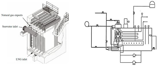
Figure 12.
Schematic diagram of the structure of ORV and SCV.
Vaporizer equipment may suffer from aging and reduced heat transfer efficiency. Regular cleaning and maintenance of ORV heat exchange tubes are conducted using advanced online cleaning technologies that remove fouling without interrupting operation, improving heat transfer efficiency by approximately 10–15%. The combustion system of SCV is upgraded with high-efficiency burners and advanced combustion control technologies, such as automatic air-fuel ratio adjustment, ensuring more complete combustion and thereby enhancing vaporization efficiency while reducing energy consumption.
In the gasification process, LNG will release a large amount of cold energy, and the addition of cold energy recovery devices and waste heat recovery systems can improve the energy utilization efficiency of the receiving station. Through the simulation analysis of HYSYS software, the cold energy recovery device can reduce the energy consumption in the air separation process by about 30–40% by using LNG cold energy for air separation. When used for power generation, the comprehensive energy utilization efficiency can be improved by about 5–10%. The waste heat recovery system uses the waste heat generated by the SCV to preheat the LNG, which can increase the overall gasification efficiency of the vaporizer by about 5–8%.
- (3)
- Optimization of the storage process
Using the tank pressure and liquid level control system based on model predictive control (MPC), according to the LNG storage capacity, gasification export capacity, ambient temperature, and other factors, the dynamic mathematical model of the storage tank is established, as shown in Figure 13, and the real-time optimization algorithm is used to predict the change trend of tank pressure and liquid level in the future and adjust the control strategy in advance. High-precision pressure and level sensors are installed to improve the accuracy of pressure and level measurements. At the same time, the sensors are regularly calibrated and maintained to ensure the reliability of the measurement data. Precise control of tank pressure and level based on accurate measurement data avoids problems such as over- or underpressure and over-limit levels, establishing a real-time monitoring system for tumbling phenomena. Multiple temperature sensors are used to monitor the temperature at different heights and positions of the storage tank, combined with data analysis algorithms, to determine whether the LNG in the storage tank is stratified in real time. As soon as signs of stratification are recognized, precautions are taken [33]. When the tumbling phenomenon is found to be unavoidable, convection is formed in the storage tank by controlling the inlet and outflow flow and direction of the LNG to alleviate the intensity of the tumbling. At the same time, pay close attention to the pressure and liquid level changes in the storage tank to ensure the safe operation of the storage tank.
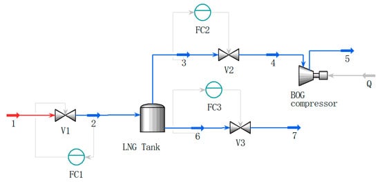
Figure 13.
Dynamic model of LNG storage tank.
The Model Predictive Control (MPC) system for the storage tank is configured as follows: Prediction horizon: 1 h (based on historical field data, pressure fluctuation within 1 h is ≤0.05 MPa); Control cycle: 10 min (the BOG compressor load is adjusted every 10 min according to prediction results); Constraints: Tank pressure is maintained between 0.5 and 0.7 MPa, and liquid level between 30 and 80%; Algorithm implementation: The controller is developed using the MATLAB R2022b MPC Toolbox. Input variables include LNG feed flow rate, send-out flow rate, and ambient temperature; output variables are BOG compressor frequency and tank inlet valve opening. Through rolling optimization, proactive control of pressure and liquid level is achieved. Compared to conventional PID control, the pressure fluctuation amplitude is reduced by 40% (from ±0.08 MPa to ±0.05 MPa).
Fault tree models were established for three types of extreme failures—“seawater pump trip,” “sudden BOG surge,” and “valve sticking”. The safety response logic (ESD/PSD interlock) was validated through dynamic simulation in HYSYS. The results are summarized in Table 11.
Table 11.
Extreme Scenario Simulation and Safety Response Results.
4. Conclusions
Based on Aspen HYSYS, a process model of the LNG terminal was developed to analyze the impact of different operating conditions on energy consumption. An energy consumption optimization model for each process section of the terminal was established, and the Particle Swarm Optimization (PSO) algorithm was applied to optimize energy use. The main conclusions are as follows:
- (1)
- The developed HYSYS dynamic model was thoroughly validated: Comparison with 30 sets of field data showed an overall relative error ≤13%, unit-level error ≤12%, and total energy consumption prediction fluctuation within ±4.2% at a 95% confidence interval, meeting engineering requirements.
- (2)
- Significant multivariable interaction effects were identified: Under the combination of low seawater temperature (18 °C) × high methane content (90%) × high send-out pressure (9700 kPa), the total energy consumption was 6.2% lower than the sum of single-factor effects, providing a new direction for operational optimization.
- (3)
- The optimized solution balances energy efficiency and safety: By expanding the objective function (incorporating start-stop frequency and flare emissions) and applying explicit constraints (NPSH margin, two-phase flow avoidance), total energy consumption was reduced by 18.5%, while equipment start-stop cycles and flare emissions were reduced by 60% and 52%, respectively.
- (4)
- Process optimization ensured controllable safety: Intelligent precooling with phased temperature drop control (rate ≤ 5 °C/min) eliminated thermal stress risks. Under extreme conditions, the safety response time was ≤ 8 s, effectively preventing accidents such as overpressure and liquid hammer.
Author Contributions
Conceptualization, H.H. and X.L.; methodology, T.W.; software, Z.Y.; data curation, J.L. and W.Y.; writing—original draft preparation, W.D. writing—review and editing, W.D. and J.L.; supervision, J.L.; funding acquisition, J.L. All authors have read and agreed to the published version of the manuscript.
Funding
This research was funded by the Scientific Research Fund of the 646 Liaoning Provincial Department of Education, grant number LJ212410148047; Basic research project of Liaoning Provincial Department of Education: The effectiveness and mechanism of activated peroxymonosulfate system for the oxidation and removal of petroleum hydrocarbons from soil. grant number LJKMZ20220740.
Data Availability Statement
The raw data supporting the conclusions of this article will be made available by the authors on request.
Conflicts of Interest
Authors Hua Huang, Xinhui Li, Zhichao Yuan, Teng Wu, Weibing Ye were employed by the company China Transocean Natural Gas Co., Ltd. The remaining authors declare that the research was conducted in the absence of any commercial or financial relationships that could be construed as a potential conflict of interest.
References
- Ramsay, M. Collaborative innovation key to LNG fuelling automation. LNG J. 2025. Available online: https://lngjournal.com/index.php/the-journal/item/113144-collaborative-innovation-key-to-lng-fuelling-automation (accessed on 14 September 2025).
- Yang, Y.; Chen, T.; Zhang, K. Dynamic response analysis of the tank front platform in the LNG terminal under blast loading. J. Phys. Conf. Ser. 2025, 3021, 012056. [Google Scholar] [CrossRef]
- Du, Y.; Yu, Z.; Sun, W.; Yang, C.; Wang, H.; Zhang, H. Chemical looping combustion-driven cooling and power cogeneration system with LNG cold energy utilization: Exergoeconomic analysis and three-objective optimization. Energy 2024, 295, 130877. [Google Scholar] [CrossRef]
- Cao, S.; Luan, T.; Zuo, P.; Si, X.; Xie, P.; Guo, X. Simulation and Economic Benefit Analysis of Carburetor Combined Transport in Winter at a Liquefied Natural Gas Receiving Station. Energies 2025, 18, 276. [Google Scholar] [CrossRef]
- Kschammer, K. Guidance for the Sustainable and Long-term Use of LNG Terminal Sites as Logistics Hubs for Hydrogen and Its Derivatives. Energy Technol. 2025, 13, 2300969. [Google Scholar] [CrossRef]
- Srilekha, M.; Dutta, A. Design and optimization of boil-off gas recondensation process by recovering waste cold energy in LNG regasification terminals. Chem. Eng. Res. Des. 2024, 205, 292–300. [Google Scholar] [CrossRef]
- Naveiro, M.; Romero Gómez, M.; Arias-Fernández, I.; Insua, Á.B. Energy, exergy, economic and environmental analysis of a regasification system integrating simple ORC and LNG open power cycle in floating storage regasification units. Brodogradnja 2023, 74, 39–75. [Google Scholar] [CrossRef]
- Jiang, Q.; Wan, S.; Pan, C.; Feng, G.; Li, H.; Hao, F.; Hansheng, F.; Meng, B.; Meng, B.; Gu, J.; et al. Thermodynamic design and analysis of air-liquefied energy storage combined with LNG regasification system. Int. J. Refrig. 2024, 160, 329–340. [Google Scholar] [CrossRef]
- Qi, Y.; Zuo, P.; Wang, D.; Cai, Z.; Guo, Y. Multi-Port Converter Design Solution for LNG Cold Power Generation. In Proceedings of the 3rd Asia Power and Electrical Technology Conference (APET), Fuzhou, China, 15–17 November 2024; pp. 632–635. [Google Scholar] [CrossRef]
- Wan, Q.; Liu, S.; Feng, D.; Huang, X.; Alotabi, M.A.; Liu, X. Optimizing trigeneration energy systems: Biogas-centric methanol production via direct CO2 hydrogenation with advanced integration of PEM electrolyzer and LNG cold technology. Sci. Total Environ. 2024, 954, 176206. [Google Scholar] [CrossRef]
- Abibou, S.; El Bourakadi, D.; Yahyaouy, A.; Gualous, H. Optimizing Hydrogen Refueling Station Recommendations: A Comparative Analysis Between Genetic Algorithm and Particle Swarm Optimization. SN Comput. Sci. 2024, 5, 991. [Google Scholar] [CrossRef]
- Qi, G.; Luo, X.; Men, C.; Li, C. Research on Optimal Control Strategy for Hydroelectric Units Based on Generalized Smith Predictor and Shortest Time Control. J. Phys. Conf. Ser. 2024, 2854, 012087. [Google Scholar] [CrossRef]
- Li, B.; Xiem, H.; Sun, L.; Gao, T.; Xia, E.; Liu, B.; Wang, J.; Long, X. Advanced exergy analysis and multi-objective optimization of dual-loop ORC utilizing LNG cold energy and geothermal energy. Renew. Energy 2025, 239, 122164. [Google Scholar] [CrossRef]
- Syauqi, A.; Uwitonze, H.; Chaniago, Y.D.; Lim, H. Design and optimization of an onboard boil-off gas re-liquefaction process under different weather-related scenarios with machine learning predictions. Energy 2024, 293, 130674. [Google Scholar] [CrossRef]
- Zhang, Z.; Li, Z.Y.; Wang, Q.; Wang, Z.; Gong, L.; Wang, B. A study on the scheme of cold energy recovery for compensating liquefaction in liquid hydrogen energy storage. IOP Conf. Ser. Mater. Sci. Eng. 2025, 1327, 012090. [Google Scholar] [CrossRef]
- Venkataramanan, V.S.; Srinivasan, R. Supply Chain Risk Management in LNG Import Terminals through Proactive and Reactive Operational Strategies. Ind. Eng. Chem. Res. 2024, 63, 19. [Google Scholar] [CrossRef]
- Yuan, W.; Yin, Z.; Su, Y.; Liu, Z.; Bao, L.; An, J. Design and Energy-Saving Analysis of a New LNG Vaporizer Based on Mg-Based Hydrogen Storage Metal. Energies 2025, 18, 875. [Google Scholar] [CrossRef]
- Dirik, C.; Biak, D.R.B.; Razak, M.B.A.; Ibrahim, N.N.L.N. Flooding Probability in Temporal Risk Assessment for LNG Vaporizer Unit Established in West Coast Malaysia. IDRiM J. 2025, 15, 1–20. [Google Scholar] [CrossRef]
- South, D.W. Methane Emissions from Oil and Natural Gas Operations—30 Percent Reduction by 2030 Possible if Domestic and International Actions “Stay the Course”. Clim. Energy 2024, 41, 22–27. [Google Scholar] [CrossRef]
- Jeon, G.M.; Park, J.C.; Choi, S. Multiphase-thermal simulation on BOG/BOR estimation due to phase change in cryogenic liquid storage tanks. Appl. Therm. Eng. 2020, 184, 116264. [Google Scholar] [CrossRef]
- Jena, P.; Singh, R.K.; Lal, V.N. Improving Light-Load Performance in Bidirectional AC–DC DAB Using Asymmetric Semivariable Frequency Modulation. IEEE Trans. Power Electron. 2025, 40, 7015–7028. [Google Scholar] [CrossRef]
- Li, R.; Tang, F.; Pan, J.; Cao, Q.; Hu, T.; Wang, K. Energy integration of LNG cold energy power generation and liquefied air energy storage: Process design, optimization and analysis. Energy 2025, 321, 135513. [Google Scholar] [CrossRef]
- Ztekin, R.; Sponza, D.T. Energy Minimization in CO2 Capture in a Natural Gas Power Plant. In Energy and Sustainable Aviation Fuels Solutions, Proceedings of the International Symposium on Sustainable Aviation 2023, Tainan, Taiwan, 26–28 July 2023; Karakoc, T.H., Jan, S.S., Wu, C.Y., Gaetano, C., Dalkiran, A., Ercan, A.H., Eds.; Springer: Cham, Switzerland, 2025. [Google Scholar] [CrossRef]
- Li, B.; Guo, Z.; Zheng, L.; Du, M.; Han, J.; Yang, C. Effect of modified eva-gmx bionic nanocomposite pour point depressants on the rheological properties of waxy crude oil. Fuel 2026, 403, 136025. [Google Scholar] [CrossRef]
- Zhao, Y.; Qian, C.; Wu, Z.; Zhang, B.; Wu, H.; Xia, H. Development of a rapid analysis system for pre-cooling process of large LNG full-capacity storage tank. J. Phys. Conf. Ser. 2024, 2845, 012049. [Google Scholar] [CrossRef]
- Abdel-Salam, M.; Askr, H.; Hassanien, A.E. Adaptive chaotic dynamic learning-based gazelle optimization algorithm for feature selection problems. Expert Syst. Appl. 2024, 256, 124882. [Google Scholar] [CrossRef]
- Ghorpade, S.N.; Zennaro, M.; Chaudhari, B.S.; Saeed, R.A.; Alhumyani, H.; Abdel-Khalek, S. Enhanced Differential Crossover and Quantum Particle Swarm Optimization for IoT Applications. IEEE Access 2021, 9, 93831–93846. [Google Scholar] [CrossRef]
- Bawa, S.; Rana, P.S.; Tekchandani, R.K. Migration of containers on the basis of load prediction with dynamic inertia weight based PSO algorithm. Clust. Comput. 2024, 27, 14585–14609. [Google Scholar] [CrossRef]
- Ghorpade, S.N.; Zennaro, M.; Chaudhari, B.S.; Saeed, R.A.; Alhumyani, H.; Abdel-Khalek, S. A Novel Enhanced Quantum PSO for Optimal Network Configuration in Heterogeneous Industrial IoT. IEEE Access 2021, 9, 134022–134036. [Google Scholar] [CrossRef]
- Karbassi Yazdi, A.; Kaviani, M.A.; Emrouznejad, A.; Sahebi, H. A binary particle swarm optimization algorithm for ship routing and scheduling of liquefied natural gas transportation. Transp. Lett. Int. J. Transp. Res. 2019, 12, 223–232. [Google Scholar] [CrossRef]
- Venkataramanan, V.S.; Srinivasan, R. Agent-Based Dynamic Simulation for Supply Chain Management of LNG Import Terminals. Ind. Eng. Chem. Res. 2024, 63, 2750–2768. [Google Scholar] [CrossRef]
- Rinaldi, K.; Collado, A.; Trong, T.T.; Hue, O. One hour of internal precooling with cold water/menthol enhances cycling performance in a heat/wet stress environment: A pilot study. Biol. Sport 2023, 40, 477–483. [Google Scholar] [CrossRef]
- Huang, P.; Zhang, K.; Chui, T.F.M. Hydrologic performance of permeable pavements under extreme and regular rainfall conditions. J. Hydrol. 2025, 652, 132653. [Google Scholar] [CrossRef]
Disclaimer/Publisher’s Note: The statements, opinions and data contained in all publications are solely those of the individual author(s) and contributor(s) and not of MDPI and/or the editor(s). MDPI and/or the editor(s) disclaim responsibility for any injury to people or property resulting from any ideas, methods, instructions or products referred to in the content. |
© 2025 by the authors. Licensee MDPI, Basel, Switzerland. This article is an open access article distributed under the terms and conditions of the Creative Commons Attribution (CC BY) license (https://creativecommons.org/licenses/by/4.0/).