Article

Intelligent Interpretation of Sandstone Reservoir Porosity Based on Data-Driven Methods

1
College of Petroleum Engineering, Xi’an Shiyou University, Xi’an 710065, China
2
Engineering Research Center of Development and Management for Low to Ultra-Low Permeability Oil & GasReservoirs in West China, Ministry of Education, Xi’an 710065, China
3
Changqing Oilfield Company of PetroChina, Xi’an 710018, China
*
Author to whom correspondence should be addressed.
Processes 2025, 13(9), 2775; https://doi.org/10.3390/pr13092775
Submission received: 31 July 2025 / Revised: 22 August 2025 / Accepted: 27 August 2025 / Published: 29 August 2025
(This article belongs to the Section Energy Systems)

Abstract

To address the technical challenge of real-time interpretation of sandstone reservoir porosity during drilling, a data-driven approach is employed by integrating logging data with machine learning algorithms to deeply mine existing logging data and predict the porosity range of encountered reservoirs. Initially, the acquired logging data is cleaned, and correlation analysis is conducted on the feature parameters. Porosity values were discretized into intervals according to field conditions. Subsequently, porosity-intelligent interpretation models are established using One-vs.-One Support Vector Machines (OVO SVMs), Random Forest (RF), XGBoost, and CatBoost algorithms. Model parameters are optimized using grid search and cross-validation methods. Finally, the test data is interpreted based on the four models with optimized parameters. Results indicate that all four models achieve training accuracies exceeding 95% and test accuracies exceeding 85%. Considering precision, recall, and F1 score comprehensively, the RF model is selected for the case study, with all three indicators exceeding 96%. These findings demonstrate that data-driven methods based on machine learning can accurately interpret sandstone reservoir porosity within specified intervals. For porosity interpretation of sandstone reservoirs in different blocks, interpretation models should be developed using multiple machine learning algorithms, and the best performing model should be selected for practical deployment. This method can be integrated with geological steering drilling technology during horizontal well drilling to ensure that the wellbore trajectory passes through higher-quality reservoir intervals, thereby providing certain guidance for maximizing the encounter rate of reservoir sweet spots.

1. Introduction

The porosity of reservoir rocks stands as a pivotal parameter in the oil and gas industry, essential for evaluating reservoir quality and assessing hydrocarbon potential. It embodies the rock’s capacity to retain fluids and serves as a fundamental metric for reserve estimation, as well as for devising and overseeing development strategies. Conventionally, porosity measurements have been conducted through laboratory tests, density logging, neutron logging, acoustic logging, and nuclear magnetic resonance logging. Nonetheless, these methodologies are fraught with constraints, including elevated costs and vulnerability to well logging conditions and equipment. Recently, the surge in artificial intelligence and machine learning technologies has propelled the application of machine learning for predicting reservoir porosity into the forefront of research. Numerous oilfields have amassed extensive logging data; however, the utilization of this wealth of information remains constrained. The advent of big data offers a promising avenue for deeply mining and extracting valuable insights from these massive reservoir datasets.
Owing to the constraint of limited core data, an exhaustive representation of the drilled strata’s properties remains elusive. The interpretation of logging data is inherently tied to the expertise and experience of engineers [1,2]. A plethora of untapped information within log data awaits exploration. Traditional research methodologies exhibit constraints in their analytical capabilities, necessitating the incorporation of big data theory and advanced data mining techniques. Recently, advancements in statistics and computer science have facilitated the development of methods grounded in machine learning theory for predicting reservoir characteristics [3,4,5,6,7,8,9,10,11]. Simple linear models fall short in capturing the intricate nonlinear relationships inherent in geological conditions, sedimentary environments, and reservoir rock samples. Empirical formulations, while applicable to specific reservoirs, are often cumbersome to derive and time consuming, rendering them inadequate for meeting the dynamic demands of production. Pallabi Saikia conducted extensive research on the literature, focusing on various aspects of the evolution of ANN in the field of reservoir characterization over time, including its architecture, learning processes, and integration with other machine learning models to enhance its modeling capabilities. This evolution has now extended to the latest advanced techniques of ANN, and its application will contribute to the intelligent interpretation of oil reservoirs [12]. Linqi Zhu proposed a new method to form unlabeled logging big data. And, based on this, he established a semi-supervised deep learning method suitable for calculating the porosity of deep-sea gas hydrate-bearing sediments by forming a porosity evaluation model [13]. LIU Guoqiang proposed a Knowledge-Powered Neural Network Formation Evaluation model (KPNFE) based on the well logging knowledge graph of hydrocarbon-bearing formations (HBFs) [14]. Saad Alatefi integrated a large database comprising 2100 well log records and core porosity measurements and combined four state-of-the-art machine learning techniques (MLP-ANN, GPR, LS-Boost, and RBF-NN) to predict reservoir porosity [15]. Similarly, machine learning has been well applied in other engineering fields [16,17,18,19,20,21,22,23,24,25,26,27,28].
It is evident that machine learning has demonstrated excellent performance in the interpretation of reservoir porosity, with different algorithms possessing their respective advantages and characteristics. This paper conducts an analysis of data from a research area in the Yanchang Oilfield using four algorithms: One-vs.-One Support Vector Machines (OVO SVMs), Random Forest (RF), XGBoost, and CatBoost. The research focuses on data-driven intelligent interpretation of porosity.

2. Materials and Methods

2.1. Data Preparation and Processing

In today’s data-driven intelligent applications, data preparation and processing stand as pivotal steps. These procedures not only exert a direct influence on the performance of machine learning models but also dictate the models’ ability to effectively learn from the data and deliver precise predictions.
Experimental data, well logging data, and corresponding porosity results that have been accurately analyzed for the study area must be obtained. For core porosity directly measured through experimental means, it is necessary to collect well logging data from the coring location. For porosity obtained through traditional methods based on well logging data, as much multi-source well logging information as possible must be collected.
Data processing typically consists of two steps: the first step is data cleaning, and the second step is data normalization. In practical field logging operations, inherent uncertainties exist that cannot fully assure the accuracy and reliability of the acquired logging data. Anomalies or missing values may arise, and if left uncorrected or unremoved, they can significantly impair the practical applicability and precision of subsequent models. Consequently, it becomes imperative to undertake a rigorous data cleaning process on the extensive volume of collected logging data. The primary objectives of logging data cleaning encompass completing incomplete records, rectifying erroneous entries, and eliminating duplicated information.
Prior to data analysis, it is customary to standardize the data. The purpose of data standardization is to rescale the data such that it fits within a narrow, specified range. This process eliminates the unit constraints of the data and transforms it into a dimensionless, pure numerical form, thereby enabling the comparison and weighting of indicators with disparate units or magnitudes. Various methods exist for data standardization, including min–max normalization, Z-score normalization, and decimal scaling normalization. In this study, we employ min–max normalization, as delineated by Formula (1), to standardize the logging data:
x i = x i x m i n x m a x x m i n
where x m a x is the maximum value of the sample data; x m i n is the minimum value of the sample data.
Various logging principles encompass a wide range of logging techniques, and the execution of logging operations often requires the synergistic application of multiple methods rooted in diverse principles. Consequently, certain logging datasets may display substantial correlations. In the absence of rigorous feature parameter analysis and selection, this intercorrelation can markedly influence the precision and computational efficiency of subsequent machine learning model training endeavors. If there is a high correlation between two or more features, redundant features can be removed to reduce model complexity, avoid overfitting, and improve computational efficiency. Through correlation analysis, feature parameters that are highly correlated with the target variable can also be identified, allowing for the selection of the most helpful features for prediction and enhancing model accuracy.

2.2. Selection of Machine Learning Algorithms

Machine learning techniques can be employed to interpret reservoir characteristics during the drilling process [29]. The efficacy of various algorithms varies depending on the volume of sample data and the nature of the feature parameters. Given the inherent challenges and complexities associated with porosity interpretation, this study selects four advanced algorithms: One-Versus-One Support Vector Machines (OVO SVMs), Random Forest (RF), eXtreme Gradient Boosting (XGBoost), and Categorical Boosting (CatBoost).

2.2.1. One-Versus-One Support Vector Machines (OVO SVMs)

SVMs originate from the notion of an optimal classification hyperplane in scenarios in which data is linearly separable. The central tenet of SVMs is that this optimal hyperplane can precisely delineate between two distinct sample classes while simultaneously maximizing the distance (or margin) between them. The underlying principle of the OVO SVM algorithm entails the formulation of an SVM classifier for each possible pair of sample classes. In the context of a dataset comprising k classes, it becomes necessary to construct k(k − 1)/2 SVM classifiers, with each classifier being tasked with differentiating between a specific pair of classes [30]. During the classification of an unknown sample, all classifiers are invoked to assign it to a particular class, and a majority voting mechanism is employed to determine the ultimate classification.

2.2.2. Random Forest (RF)

RF is a supervised learning algorithm that falls within the realm of ensemble learning methods, primarily employed for both classification and regression tasks. By constructing a multitude of decision trees and aggregating their predictive outputs, RF significantly bolsters the model’s overall accuracy and robustness. This algorithm demonstrates exceptional proficiency in managing high-dimensional data, efficiently training and generating predictions even in the presence of a substantial number of features [7]. Additionally, RF possesses the capability to adeptly handle partially missing values during the training phase, thereby producing reliable predictive outcomes even with incomplete datasets. Notably, RF is characterized by a relatively modest number of hyperparameters that exhibit low sensitivity, with the default settings frequently leading to satisfactory performance.

2.2.3. eXtreme Gradient Boosting (XGBoost)

XGBoost is an advanced ensemble learning algorithm grounded in Gradient Boosting Decision Trees (GBDTs), designed to forge a robust integrated model by amalgamating multiple weak learners. Building upon the foundation of GBDT, XGBoost introduces an array of optimizations to elevate model performance and expedite training. In contrast to conventional GBDTs, which solely harnesses first-order derivative information, XGBoost incorporates second-order derivative data to refine the loss function optimization. This incorporation leads to a more precise approximation of the loss function and accelerates convergence towards the optimal solution. To mitigate the risk of overfitting, XGBoost integrates regularization terms into the objective function, encompassing subsample, colsample_bytree, and the maximum depth of trees (max_depth). These regularization components serve to constrain model complexity and enhance the model’s generalization capability.
Furthermore, XGBoost is engineered to support parallel processing, harnessing the power of multi-core processors to substantially accelerate the model training process. It efficiently organizes data through a Block storage structure, facilitating seamless parallel computation.

2.2.4. Categorical Boosting (CatBoost)

CatBoost is a decision tree algorithm based on gradient boosting, particularly adept at handling datasets containing numerous categorical features. It is grounded in the framework of gradient boosting, which means it iteratively constructs multiple decision trees to progressively reduce prediction errors. Each tree is built upon the prediction residuals of all the preceding trees, aiming for the new tree to correct as many prediction errors as possible from the earlier ones. A distinctive aspect of CatBoost lies in its special handling of categorical features, marking a significant departure from other gradient boosting algorithms. In traditional gradient boosting algorithms, categorical features often need to be converted into numerical features through methods such as one-hot encoding. However, CatBoost can directly process categorical features without requiring complex preprocessing.
CatBoost employs a technique known as “target statistics” or “feature importance” to deal with categorical features. For each categorical feature, CatBoost calculates the category distribution corresponding to each category and utilizes these statistics as new numerical features. Additionally, CatBoost adopts the technique of ordered boosting to avoid the issue of prediction shift. In traditional gradient boosting, the same set of features is used for each sample when constructing trees. However, in CatBoost, samples are randomly ordered, and when constructing each tree, only the feature values of samples ranked before the current sample are used to compute the prediction for the current sample. This approach ensures that the model does not “peek” at future data during training, which improves generalization.

2.3. Establishment of Intelligent Interpretation Model for Porosity

In the establishment of a porosity interpretation model utilizing OVO SVMs, the two pivotal parameters requiring optimization are the regularization parameter, denoted as C, and the kernel parameter, exemplified by γ in the context of the Radial Basis Function (RBF) kernel. The regularization parameter C serves as a mechanism to regulate the model’s complexity. Specifically, a higher value of C imposes a stricter penalty on errors, rendering the model more susceptible to overfitting. Conversely, a lower value of C relaxes the penalty on errors, thereby augmenting the risk of underfitting. The kernel parameter, exemplified by γ in the RBF kernel, dictates the transformation of data into a high-dimensional feature space, consequently shaping the model’s classification performance. To achieve optimal parameter settings, grid search methodologies can be employed for the fine-tuning of these two critical parameters.
In the establishment of a porosity interpretation model utilizing RF, two pivotal parameters, namely, n_estimators and max_features, are primarily considered. The parameter n_estimators denotes the total number of decision trees in the forest. A higher value of n_estimators generally leads to improved model performance, albeit at the expense of increased computational time. Conversely, the parameter max_features specifies the upper limit on the number of features that the RF algorithm is permitted to evaluate for splitting at each node within a single tree, essentially representing a randomly selected subset of the feature set. A reduction in the size of this subset typically results in a faster decrease in variance, but concurrently, the bias may increase significantly. To determine the optimal parameter settings for the porosity interpretation model, a combination of grid search and k-fold cross-validation is employed.
In the establishment of a porosity interpretation model utilizing XGBoost, three pivotal parameters are preferentially considered: n_estimators, max_depth, and learning_rate. The parameter n_estimators denotes the number of decision trees, which is synonymous with the total number of boosting iterations. The parameter max_depth specifies the maximum depth to which each decision tree can grow; a larger value increases the risk of overfitting, whereas a smaller value elevates the likelihood of underfitting. The learning_rate parameter governs the magnitude of the step taken in each iteration to update the model weights; a smaller value results in a more gradual learning process and consequently slower training speed. To ascertain the optimal configuration of parameters for the XGBoost porosity interpretation model, a rigorous approach combining grid search and k-fold cross-validation methods is employed.
In the establishment of a porosity interpretation model utilizing CatBoost, three pivotal parameters are preferentially considered: iterations, depth, and learning_rate. The parameter iterations denotes the maximum number of decision trees to be constructed, also referred to as the number of weak estimators. Augmenting the number of iterations typically enhances the model’s fitting capability; however, an excessively high number of trees may result in overfitting and escalate computational expenses. The learning_rate parameter serves a function analogous to that in XGBoost, regulating the step size for updating model weights in each iteration. The depth parameter specifies the depth of each decision tree, where deeper trees possess the capacity to capture more-intricate patterns but also carry an increased risk of overfitting.

3. Case Study

3.1. Data Acquisition and Data Cleaning

The wells in the dataset are situated in the Qisheng wellblock of the Yanchang Oilfield in China, which is located within the Ordos Basin. A total of 18,193 sets of logging data were collected, each comprising 11 types of logging sequences: deep investigate induction log (ILD), medium investigate induction log (ILM), eight-lateral log (LL8), spontaneous potential log (SP), microgradient log (ML1), micropotential log (ML2), true formation resistivity log (RT), flushed zone resistivity log (RXO), apparent resistivity curve measured with a 0.5 m potential electrode system (R0.5), acoustic log (AC), and gamma ray log (GR). Initially, the dataset was cleaned using Python (Python version 3.12.7), and the min–max normalization method was applied for normalization, resulting in 13,249 valid data sets. A partial display of the data is presented in Table 1.
After statistical analysis, it was found that the majority of effective well logging data for the reservoir in the well area corresponds to porosities less than 30%. The porosity values in this region exhibit a mean of 10.03% and a standard deviation of 2.587. In the subsequent phases of reservoir development, porosity emerges as a pivotal factor in the assessment of reservoir sweet spots. The porosity values were categorized into seven distinct classes: type 1 ((0.1%, 4%)), type 2 ([4%, 8%)), type 3 ([8%, 12%)), type 4 ([12%, 16%)), type 5 ([16%, 20%)), type 6 ([20%, 24%)), and type 7 (≥24%).

3.2. Correlation Analysis

Incorporating a greater variety of data types and feature parameters does not necessarily ensure enhanced machine learning accuracy. Well logging data often contain some noise, which can exert an influence on the outcomes of machine learning identification processes. Well logging data obtained through similar logging principles often exhibit strong correlations. If the data volume is too large or the correlation among characteristic parameters is high, a parameter redundancy phenomenon can occur. This phenomenon not only prolongs the machine learning computation time but may also detrimentally impact the precision of model training. Consequently, it is imperative to conduct a thorough correlation analysis of the collected logging data.
A comprehensive correlation analysis was performed on 11 distinct types of log data. As depicted in Figure 1, a notably strong correlation was observed between ILM and ILD. LL8 demonstrated a correlation coefficient exceeding 0.5 with both ILM and ILD. Similarly, RT and RXO exhibited a correlation coefficient greater than 0.9, while both RT and RXO showed a correlation exceeding 0.7 with ILM and ILD. Furthermore, R0.5 displayed a correlation coefficient above 0.5 with ILM, ILD, LL8, and RXO. The correlation between ML1 and ML2 was found to be approximately 0.9. Based on these findings, the logs of LL8, SP, GR, AC, RT, R0.5, and ML1 were selected as the characteristic parameters for the subsequent model establishment.

3.3. Intelligent Interpretation Model of Porosity Based on Different Algorithms

The workflow diagram for interpretation the porosity in this paper is shown in Figure 2.
The porosity interpretation model programs in this paper were all written in the Python language. The Python syntax is simple and clear, with rich and powerful libraries. This study mainly uses the scikit-learn Python framework (Python version 3.12.7). Scikit-learn is a Python module that integrates a wide range of machine learning algorithms for both supervised and unsupervised problems [31].

3.3.1. The OVO SVM Porosity Interpretation

In this study, the Gaussian kernel function was utilized alongside the grid search method to determine the approximate ranges for the optimal training parameters, C and γ, within the framework of OVO SVMs. Furthermore, a 10-fold cross-validation approach was employed to optimize the objective function and ascertain the most-suitable parameter values, thereby ensuring high predictive accuracy while effectively mitigating the risk of overfitting.
Take C = [10, 50, 100, 500, 900, 1500, 2000], γ = [0.0001, 0.001, 0.01, 0.1, 1] to search the ranges of the optimal parameter values in 35 combinations of (C, γ) using the grid search method. We obtain the optimal values of parameters C and γ, which are approximately 2000 and 0.001, respectively. The interpretation results for different parameter combinations of the OVO SVM model are shown in Figure 3 below.

3.3.2. The RF Porosity Interpretation

The RF model is characterized by two primary parameters. The parameter n_estimators denotes the number of trees within the forest and originates from the scikit-learn Python library. An increase in the number of trees leads to a corresponding increase in computation time, with the optimal predictive performance typically achieved at a moderate number of trees. The other parameter, max_features, signifies the maximum number of features that can be utilized by an individual decision tree, essentially representing a subset of randomly chosen feature sets. A reduction in the size of these subsets results in a faster decrease in variance, albeit accompanied by a more rapid increase in bias. To determine the approximate ranges for the optimal RF training parameters, n_estimators and max_features, the grid search method was employed.
Take n_estimators = [1, 10, 20, 30, 40, 50, 60], max_features = [1, 2, 3, 4, 5, 6, 7, 8, 9, 10] to search the ranges of the optimal parameter values in 70 combinations of (n_estimators, max_features) using the grid search method. We obtain the optimal values of parameters n_estimators and max_features, which are approximately 40 and 4, respectively. The interpretation results for different parameter combinations of RF model can be seen in Figure 4.

3.3.3. The XGBoost Porosity Interpretation

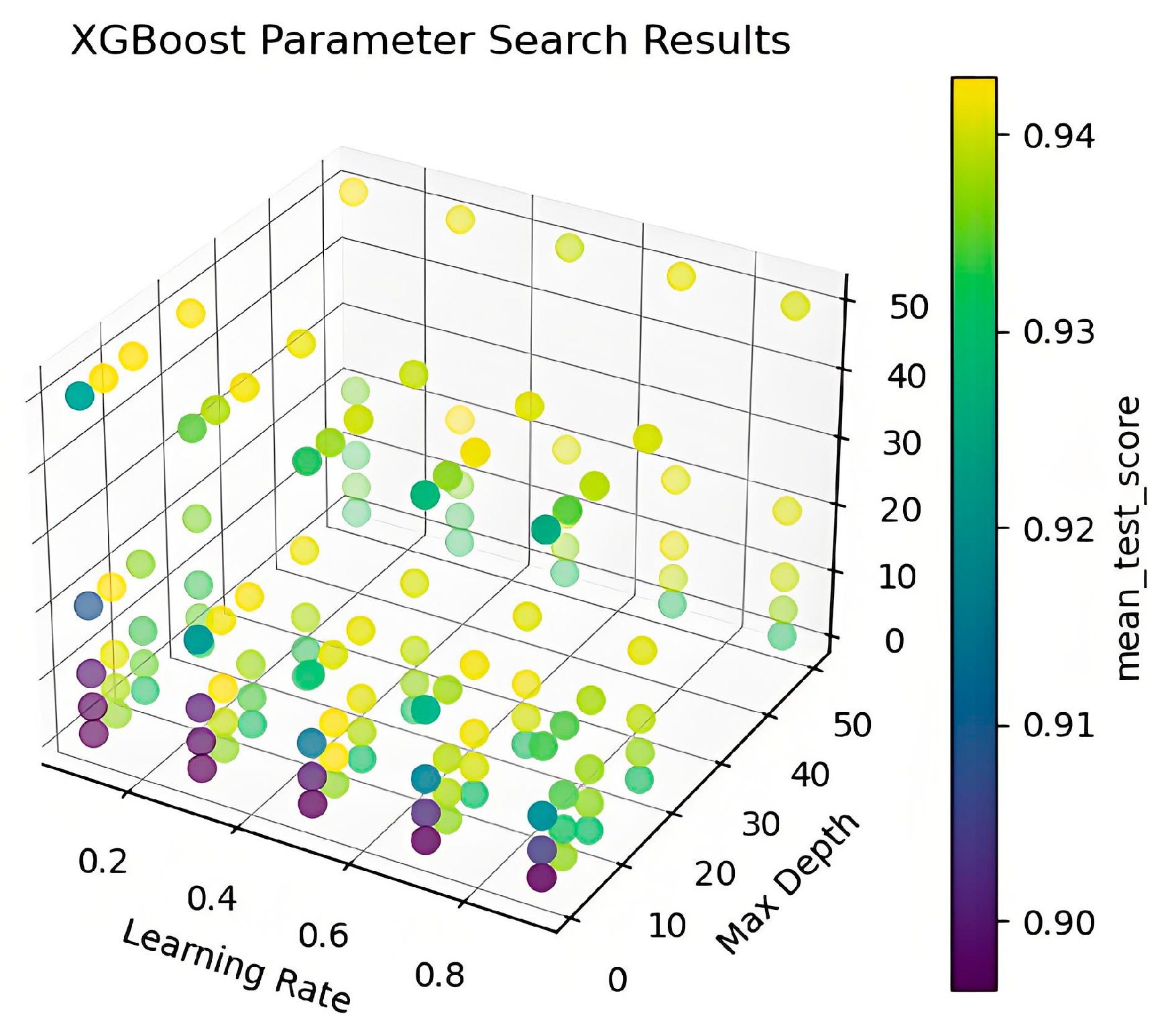
During the establishment of the XGBoost porosity interpretation model, grid search is used to optimize three main parameters.
Take n_estimators = [1, 5, 10, 20, 50], max_depth = [1, 5, 10, 20, 50], learning_rate = [0.1, 0.3, 0.5, 0.7, 0.9] to search the ranges of the optimal parameter values in 125 combinations of (n_estimators, max_depth, learning_rate) using the grid search method. We obtain the optimal values of parameters (n_estimators, max_depth, and learning_rate are approximately 20, 5, and 0.1, respectively). The interpretation results for different parameter combinations of the XGBoost model are shown in Figure 5 below.

3.3.4. The CatBoost Porosity Interpretation

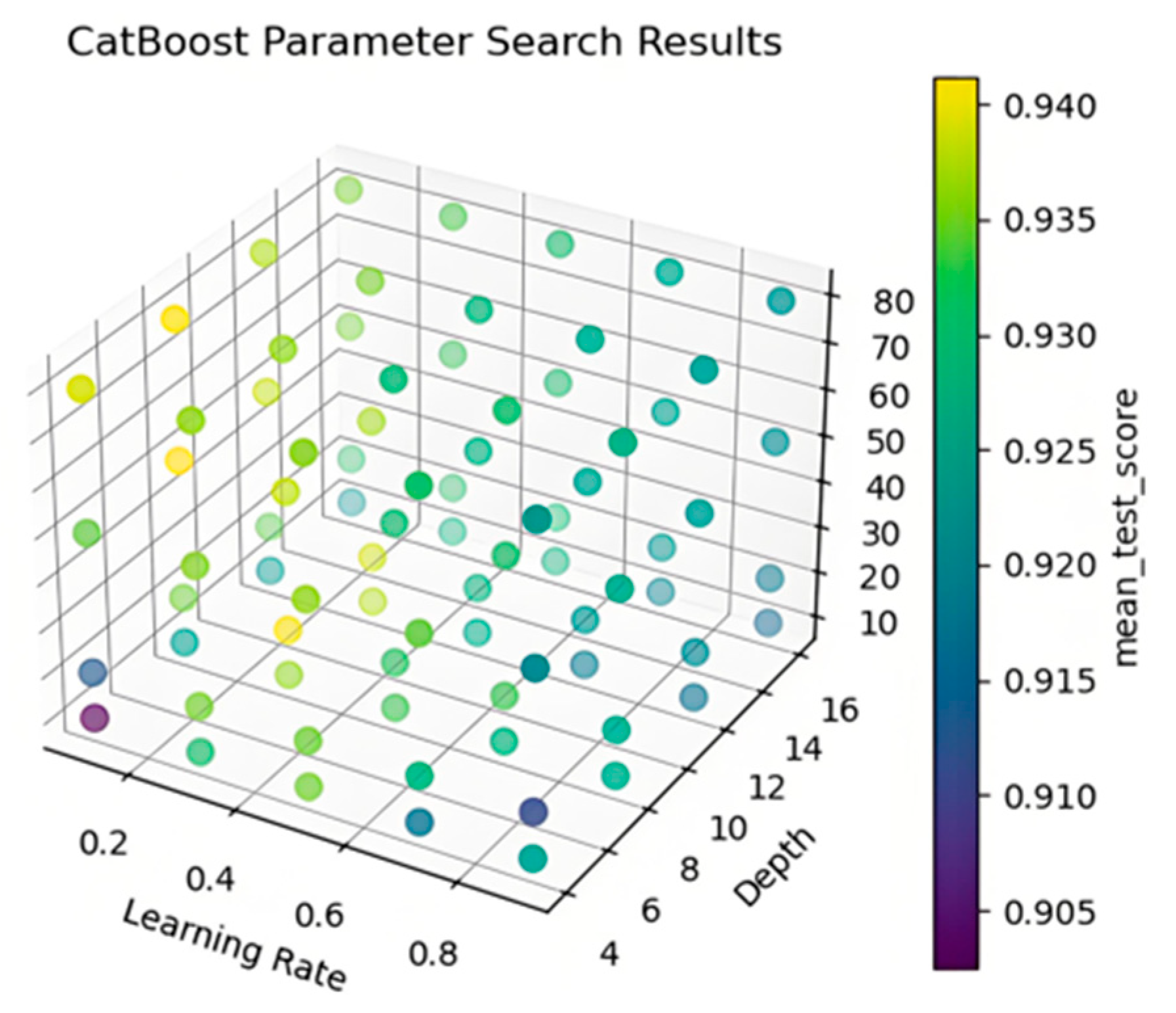
During the establishment of the CatBoost porosity interpretation model, grid search is used to optimize three main parameters.
Take iterations = [10, 20, 50, 80], depth = [4, 8, 12, 16], learning_rate = [0.1, 0.3, 0.5, 0.7, 0.9] to search the ranges of the optimal parameter values in 80 combinations of (iterations, depth, learning_rate) using the grid search method. We obtain the optimal values of parameters (iterations, depth, and learning_rate are approximately 50, 8, and 0.1, respectively). The interpretation results for different parameter combinations of the CatBoost model are shown in Figure 6 below.

3.4. Porosity Interpretation

In total, 1188 sets of logging data from the Qisheng wellblock of the Yanchang Oilfield were obtained and combined to form the test set. Then, the four interpretation models discussed above were used to interpret the porosity. The training set recognition results and test set recognition results for the four models were compared.

4. Results and Discussion

To evaluate the model’s capacity for interpreting porosity, four models with finely tuned parameters were utilized, and their performance was assessed using metrics including training set accuracy, precision score, recall score, and F1 score on the test set.
Table 2 shows the optimal parameters obtained after multiple optimizations of the four models.
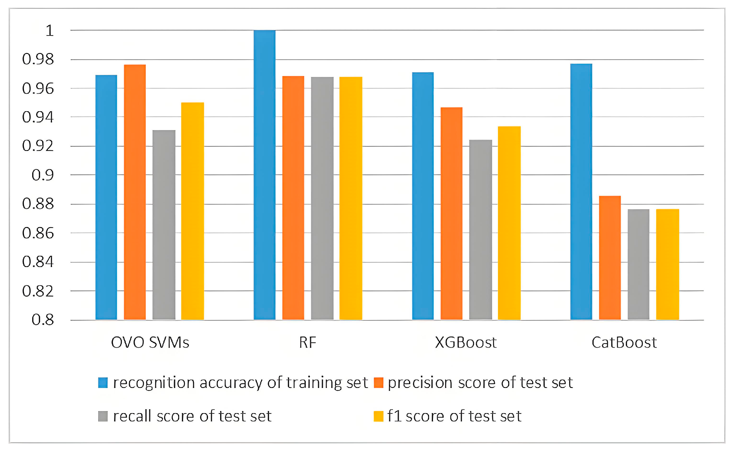
Figure 7 illustrates the recognition accuracy of the training set alongside the precision, recall, and F1 scores for the test set across four distinct models. Notably, all four models exhibit training set accuracies exceeding 96%. The RF model attains the highest recognition accuracy of 99.98%, whereas the OVO SVM model, despite having the lowest accuracy among the four, still achieves a commendable 96.94%. In terms of the test set, the OVO SVM model demonstrates the highest prediction accuracy of 97.65%; the RF model achieves the highest recall score of 96.79%; and the RF model also secures the highest F1 score of 96.81%. Conversely, the CatBoost model exhibits the lowest performance in all these evaluation metrics, with values falling below the 90% threshold. Particularly in the context of predicting reservoir porosity, the precision score and F1 score are considered crucial performance indicators and are thus emphasized.
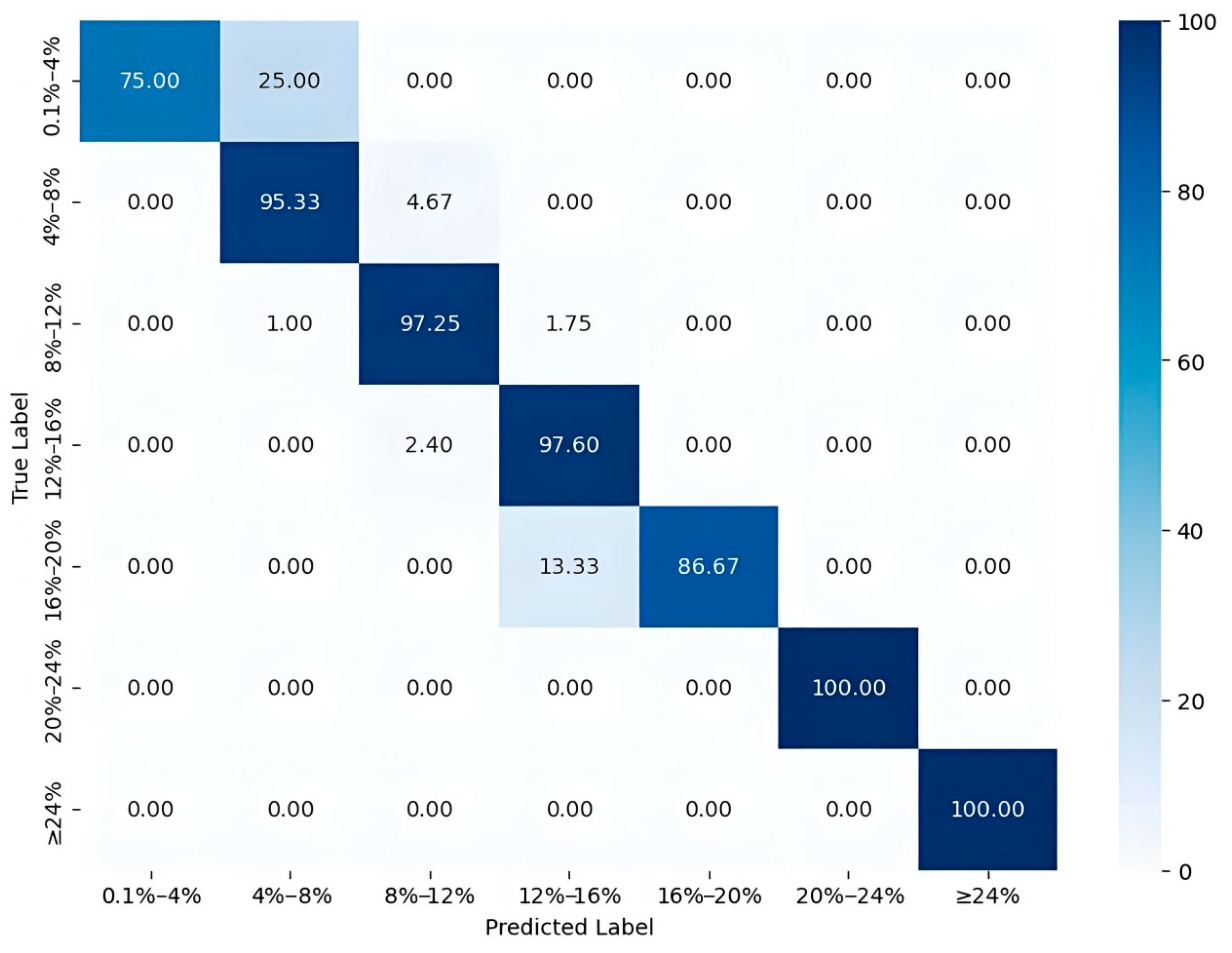
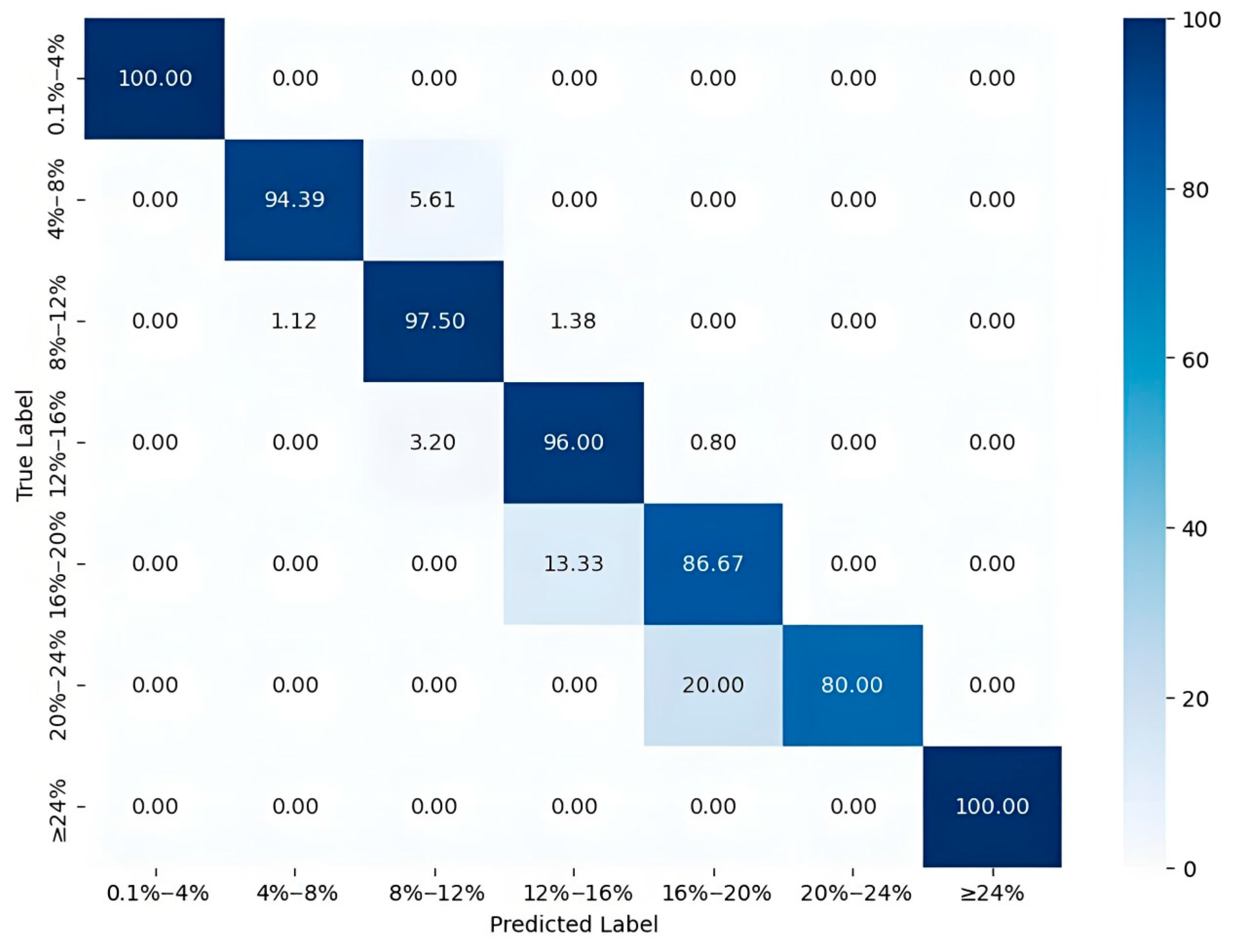
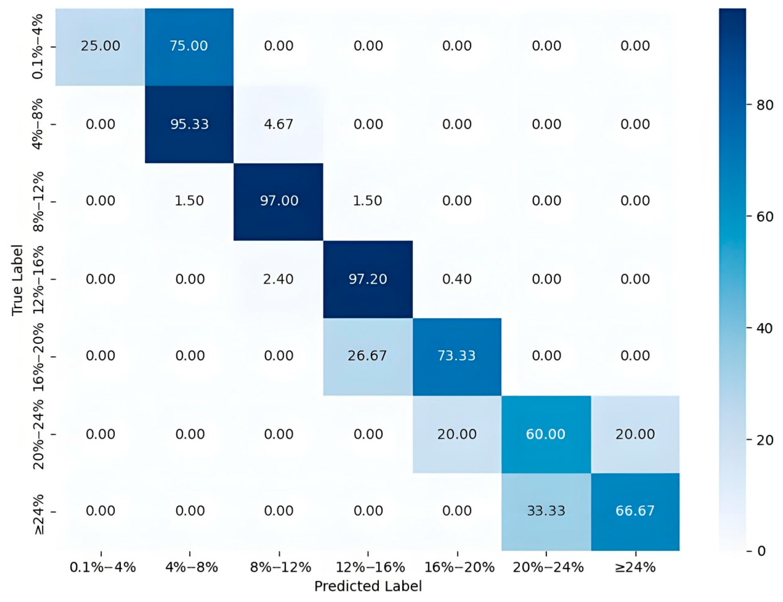
Figure 8, Figure 9, Figure 10 and Figure 11 depict the confusion matrices computed for the test set by four distinct algorithms. As illustrated in Figure 8, the OVO SVM model demonstrates a diminished prediction accuracy for reservoirs with low porosity in comparison to those with relatively higher porosity, achieving a perfect prediction accuracy of 100% solely for reservoirs with a porosity of 20%. Similarly, Figure 9 reveals that the RF model also exhibits a reduced prediction accuracy for low-porosity reservoirs when juxtaposed against higher-porosity counterparts, attaining a 100% accuracy for reservoirs with a porosity of 20%. Nonetheless, the RF model surpasses the OVO SVM model in terms of predicting low-porosity reservoirs. In contrast, Figure 10 shows a case in which the XGBoost model attains a higher prediction accuracy for low-porosity reservoirs relative to higher-porosity ones, but its accuracy decreases to below 90% for reservoirs with porosities in the range of 16% to 24%. Lastly, Figure 11 discloses that the CatBoost model solely achieves a prediction accuracy surpassing 90% for reservoirs with porosities between 4% and 16%, whereas its accuracy for reservoirs with other porosities is notably lower, rendering it the least effective model among the quartet. Collectively, all four models display superior prediction accuracies for reservoirs with porosities spanning from 4% to 16% and inferior accuracies for those with porosities ranging from 16% to 20%. Furthermore, all models exhibit a consistent trend in which they are prone to misclassify data with porosities of 16% to 20% as originating from reservoirs with porosities of 12% to 16% and incorrectly categorize data from reservoirs with porosities of 4% to 8% as belonging to those with porosities of 8% to 12%. Therefore, in the application of this case study’s region, it is imperative to allocate greater attention to the dataset in which the prediction outcomes fall within the range of 12% to 16%.
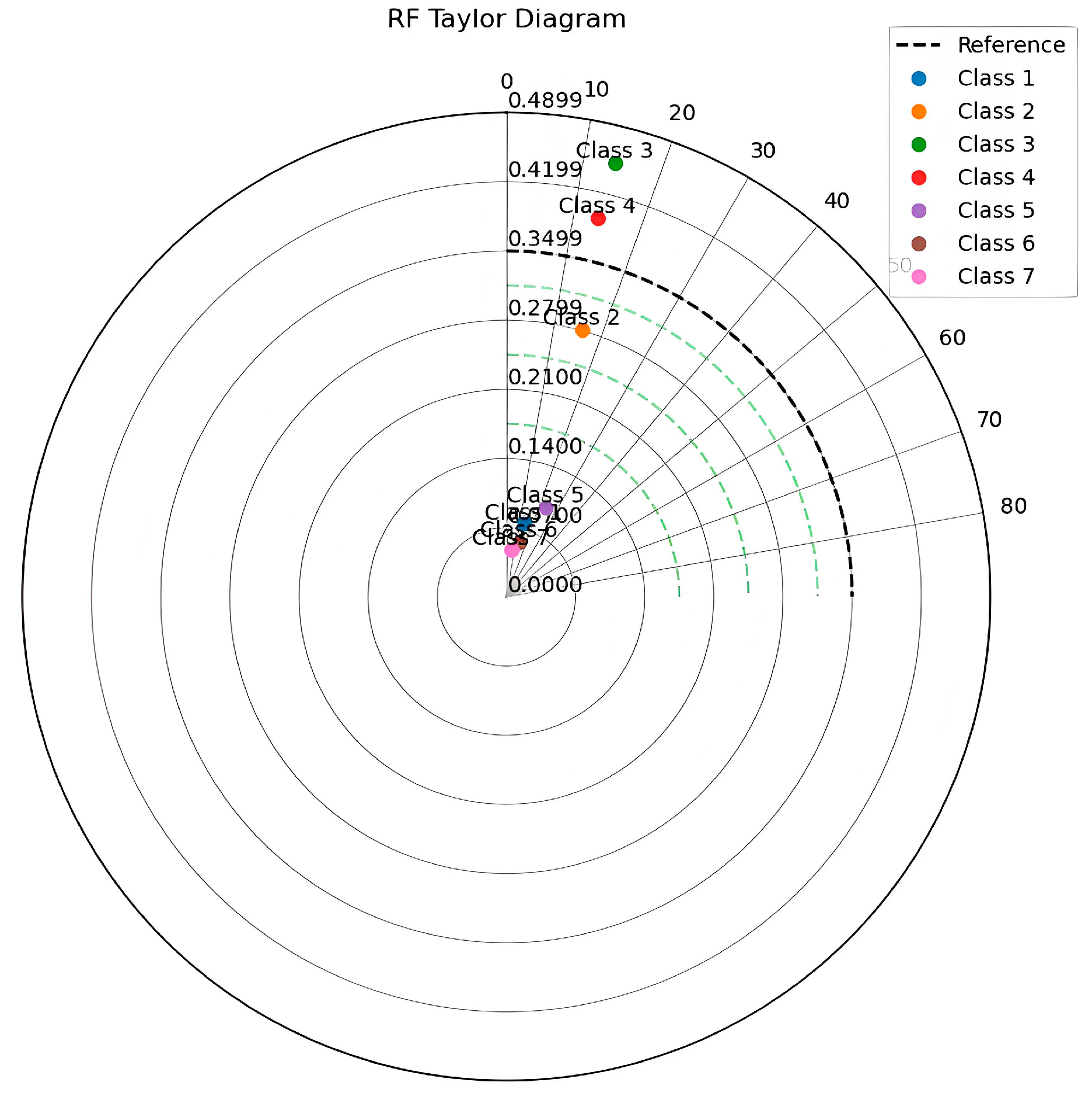
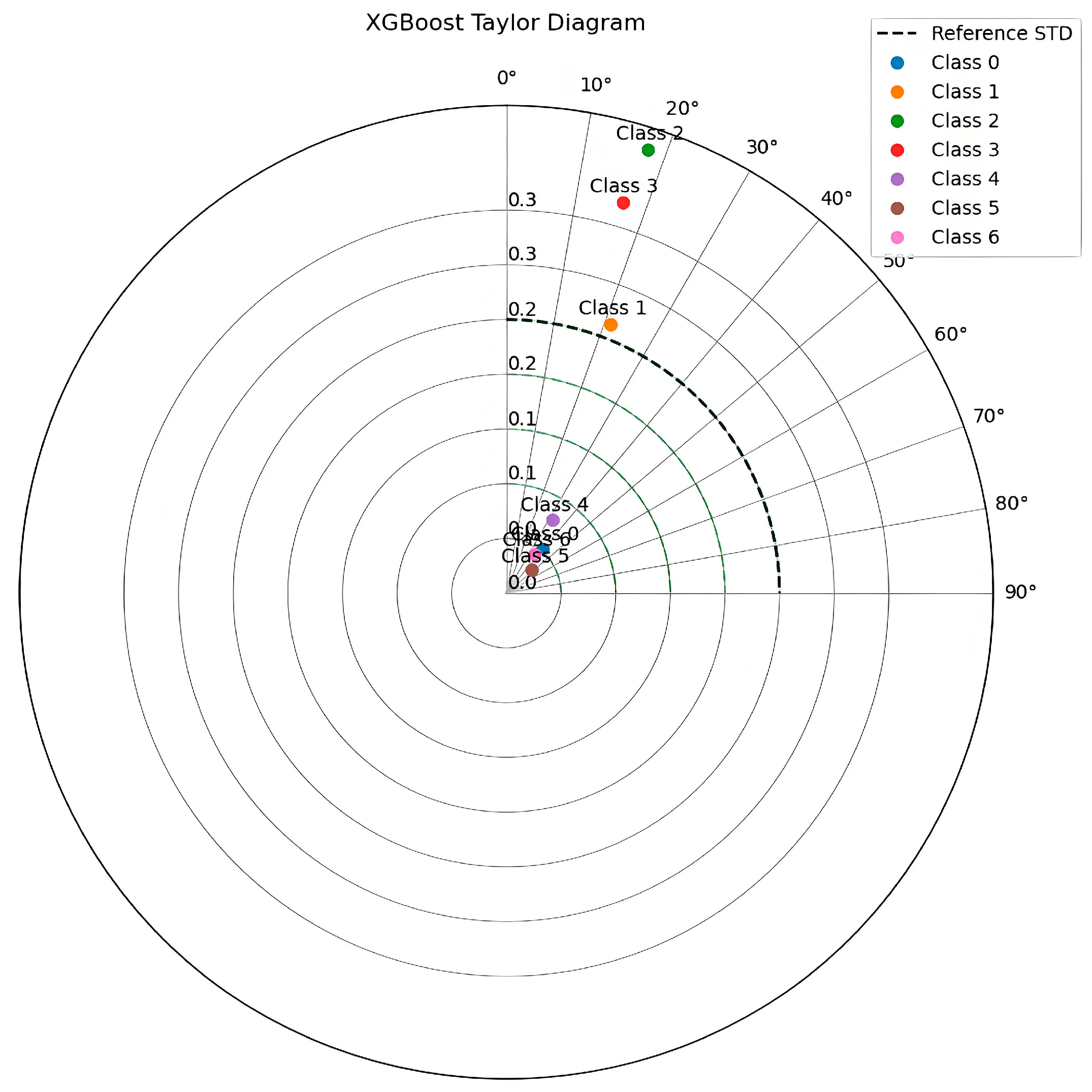
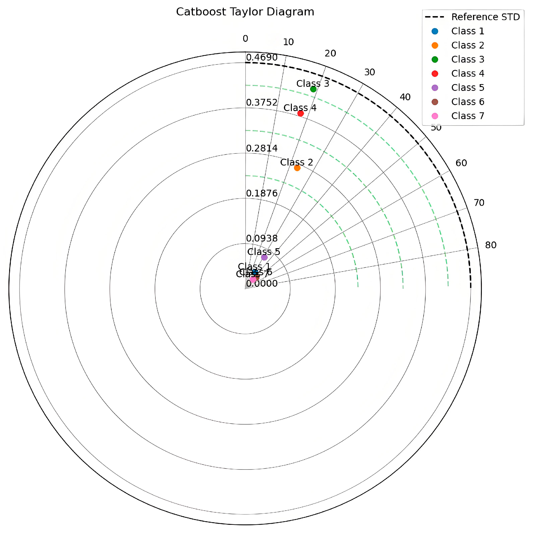
To further evaluate the performance of each model, Taylor diagrams were generated for all the models (Figure 12, Figure 13, Figure 14 and Figure 15) [32,33], and the standard deviation, correlation coefficient, and root mean square error (RMSE) for each category were calculated (Table 3, Table 4, Table 5 and Table 6). As revealed by the Taylor diagrams, the XGBoost model demonstrated superior performance, with predictions across multiple categories closely aligning with the reference line. In particular, its predictions for Class 5 and Class 6 were nearly perfect. Overall, the XGBoost model exhibited the most balanced performance and outperformed other models in most categories. The RF and CatBoost models ranked next, while the OVO SVM model performed the worst. According to the tables of standard deviation, correlation coefficient, and RMSE, the RF model achieved the best results, excelling in all three metrics. It showed particularly stable predictions, strong correlations, and low errors in Class 1, Class 6, and Class 7. The OVO SVM model achieved relatively high correlation coefficients and low RMSE in certain categories (e.g., Class 6 and Class 7). However, it exhibited high overall standard deviation, indicating considerable fluctuations in predicted values. The XGBoost model performed well in some categories (e.g., Class 2 and Class 4) but showed lower correlation coefficients and higher RMSE in Class 6 and Class 7. The CatBoost model also delivered relatively good results in certain categories (e.g., Class 2 and Class 4), but its overall performance was weaker, especially in Class 6 and Class 7.
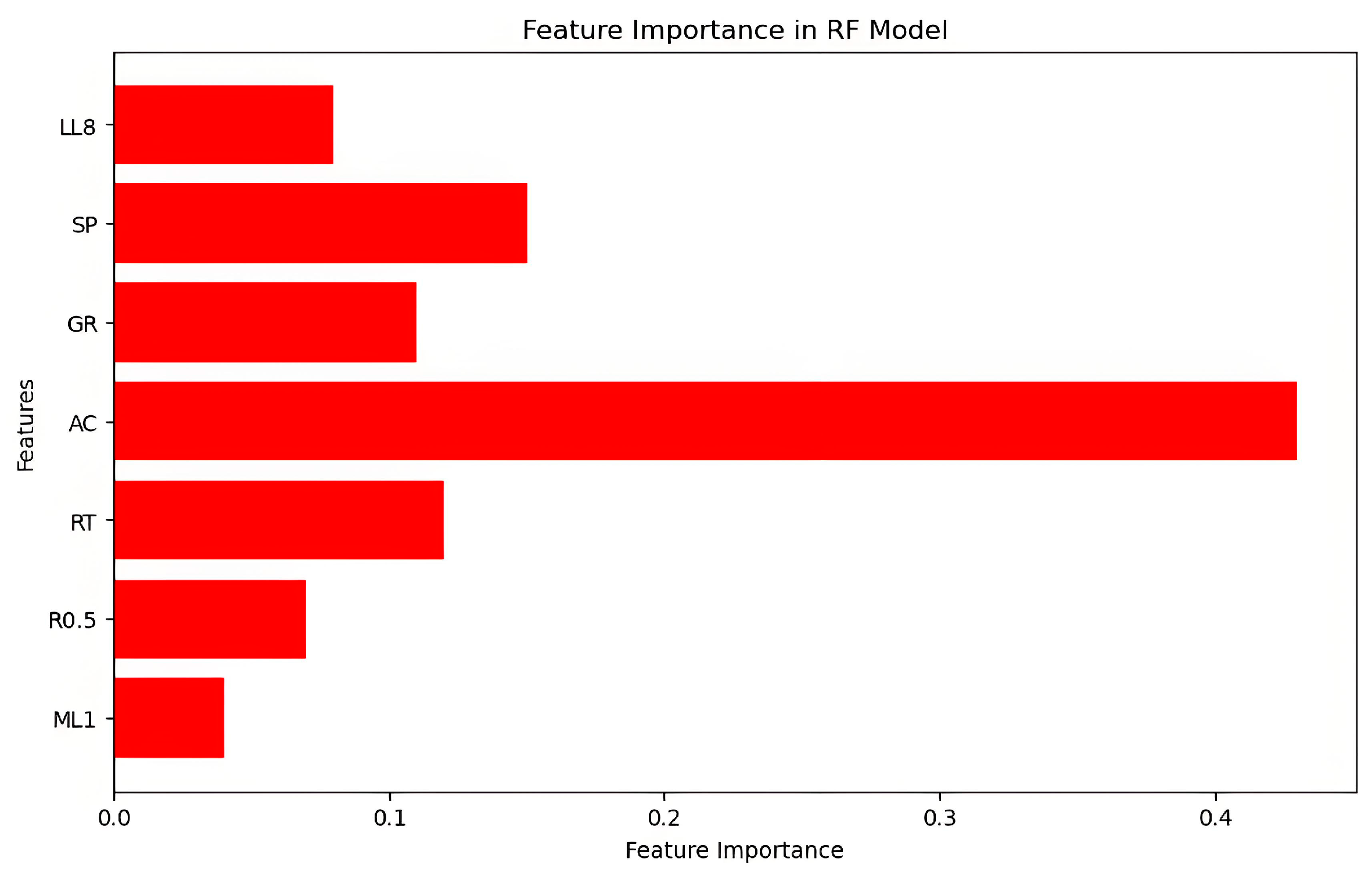
After conducting a comparative analysis of the four models’ multiple performance metrics and confusion matrices, the RF model was selected for porosity interpretation in this case study. We conducted a feature importance analysis of the RF model, and the results are presented in Figure 16. The degree of influence of each feature on the interpretation results from greatest to least is as follows: AC, SP, RT, GR, LL8, R0.5, and ML1.
By conducting a series of comparison experiments, we ascertained that the porosity interpretation model can be effectively established utilizing a data-driven methodology grounded in well logging data. The acquisition and processing of logging data form the foundation for establishing a porosity interpretation model. Serving as a sample database for model training, their accuracy is a critical factor determining the reliability of the porosity interpretation model. Consequently, during the database establishment process, meticulous data cleaning, standardization, and correlation analysis on the logging data were imperative to ensure the high application value and integrity of the database [34,35,36]. Since missing data can lead to a decline in model performance and different machine learning algorithms have varying capabilities when handling missing data, if a dataset contains a large amount of missing data, it may be necessary to select more-complex algorithms or perform additional data preprocessing, which increases both the difficulty of algorithm selection and computational costs. Noisy data can also cause model overfitting and reduce its generalizability. Therefore, before initiating model training, we cleaned the data by performing tasks such as correcting erroneous data, deleting duplicate data, and imputing missing data. Additionally, we conducted feature parameter selection through methods such as correlation analysis.
Apart from the accuracy and reliability of the database and the intrinsic performance disparities among the algorithms, another significant factor contributing to the marked differences in the recognition accuracy among the various algorithms is the selection of the feature parameters. Due to certain constraints when obtaining actual field data within the scope of this study, only a subset of the logging data was selected to provide the feature parameters. However, numerous other logging data and engineering parameters can also provide valuable insights into the characteristics of the porosity. If circumstances permit, it is advisable to consider more logging data and other engineering parameters concurrently and to expand the feature parameters for model training to further enhance the model’s predictive performance.
To achieve accurate interpretation of the porosity, it is imperative to increase the number of samples in the database and refine the classification step size for the porosity, as a reduced step size facilitates more-precise guidance for actual field development and production activities. On the basis of the case study presented, the method proposed in this paper can interpret the porosity to a certain extent, thereby offering a novel and innovative technical approach for its interpretation and evaluation.

5. Conclusions

Logging data can be used to solve nonlinear function mapping problems and interpret porosity during the drilling procedure. The intricate relationship between logging responses and the actual attributes of the reservoir often results in highly nonlinear mappings. Given the diverse range of logging response characteristics and the subdivision of reservoir porosity into multiple intervals, integrating machine learning techniques with logging data and adopting data-driven methodologies for the interpretation of reservoir porosity emerge as effective strategies to resolve this intricate problem.
This study introduces an intelligent approach for the interpretation of reservoir porosity, enabling rapid determination of porosity ranges during logging operations and offering invaluable insights for exploration and development endeavors. Compared with conventional methods, the machine learning-based approach for reservoir porosity interpretation demonstrates significant economic advantages, primarily manifested through reduced costs and enhanced efficiency. While traditional techniques rely heavily on expert knowledge and involve labor-intensive repetitive tasks, the proposed method enables automated processing and real-time analysis. Furthermore, it substantially reduces the reliance on physical experiments and specialized equipment. Leveraging four distinct machine learning algorithms, some meaningful conclusions are listed below.
(a)
Before initiating model training, conducting a thorough correlation analysis of the input data is a crucial step in avoiding data redundancy and reducing data dimensionality, thereby enhancing computational accuracy and shortening model training time.
(b)
The rational application of grid search combined with cross-validation methods for model parameter optimization is of utmost importance, as it directly influences whether the model parameter optimization can achieve a globally optimal solution rather than merely a locally optimal one.
(c)
In the reservoir case studied in this paper, through a comprehensive comparison of the recognition accuracy of the training set, precision, recall, and F1 scores of the test set, we ultimately selected the RF model as the tool for porosity interpretation. This model demonstrated the highest recognition accuracy on the training set and also achieved the highest recall and F1 scores on the test set, with a precision score exceeding 96%, showcasing exceptional performance.
(d)
Given the diverse data structures and information categories, various machine learning algorithms each exhibit their unique advantages. Therefore, when interpreting reservoir porosity in different blocks, we should construct interpretation models based on multiple machine learning algorithms and select the optimal model for practical application.
(e)
The methodology proposed in this study can be applied to other sandstone reservoirs; however, its application necessitates reconstructing the model and re-optimizing parameters using data from the new study area, reflecting certain limitations in generalizability. To address this issue, our team is currently focusing on the development of transfer learning algorithms based on an unsupervised domain adaptation framework. This method is intended to be employed in future work to interpret sandstone reservoir porosity, with the aim of enhancing the applicability of the methodology and increasing the scientific significance of related research.

Author Contributions

Methodology, J.S.; Software, Y.Z.; Validation, L.R.; Data curation, K.T.; Writing—original draft, J.S.; Visualization, Z.Z.; Funding acquisition, J.S. and Y.Z. All authors have read and agreed to the published version of the manuscript.

Funding

This research was funded by the National Natural Science Foundation of China (NSFC) (No. 52304036) and the Scientific Research Program Funded by the Shaanxi Provincial Science and Technology Department (2023-JC-QN-0432).

Data Availability Statement

The raw data supporting the conclusions of this article will be made available by the authors on request.

Conflicts of Interest

Kang Tang was employed by Changqing Oilfield Company of PetroChina. The remaining authors declare that the research was conducted in the absence of any commercial or financial relationships that could be construed as potential conflicts of interest.

References

  1. Sun, J.; Li, Q.; Chen, M.; Ren, L.; Huang, G.; Li, C.; Zhang, Z. Optimization of models for a rapid identification of lithology while drilling-A win-win strategy based on machine learning. J. Pet. Sci. Eng. 2019, 176, 321–341. [Google Scholar] [CrossRef]
  2. Sun, J.; Zhang, R.; Chen, M.; Chen, B.; Wang, X.; Li, Q.; Ren, L. Identification of Porosity and Permeability While Drilling Based on Machine Learning. Arab. J. Sci. Eng. 2021, 46, 7031–7045. [Google Scholar] [CrossRef]
  3. Zhong, Y.; Li, R. Application of Principal Component Analysis and Least Square Support Vector Machine to Lithology Identification. Well Logging Technol. 2009, 33, 425–429. [Google Scholar]
  4. Li, R.; Zhong, Y. Dentification Method of Oil/Gas/Water Layer Based on Least Square Support Vector Machine. Nat. Gas Explor. Dev. 2009, 32, 15–18+72. [Google Scholar]
  5. Song, Y.; Zhang, J.; Yan, W.; He, W.; Wang, D. A new identification method for complex lithology with support vector machine. J. Daqing Pet. Inst. 2007, 31, 18–20. [Google Scholar]
  6. Li, X.; Li, H. A new method of identification of complex lithologies and reservoirs: Task-driven data mining. J. Pet. Sci. Eng. 2013, 109, 241–249. [Google Scholar] [CrossRef]
  7. Xie, Y.; Zhu, C.; Zhou, W.; Li, Z.; Liu, X.; Tu, M. Evaluation of machine learning methods for formation lithology identification: A comparison of tuning processes and model performances. J. Pet. Sci. Eng. 2018, 160, 182–193. [Google Scholar] [CrossRef]
  8. Dong, S.; Wang, Z.; Zeng, L. Lithology identification using kernel Fisher discriminant analysis with well logs. J. Pet. Sci. Eng. 2016, 143, 95–102. [Google Scholar] [CrossRef]
  9. Othman, A.A.; Gloaguen, R. Integration of spectral, spatial and morphometric data into lithological mapping: A comparison of different Machine Learning Algorithms in the Kurdistan Region, NE Iraq. J. Asian Earth Sci. 2017, 146, 90–102. [Google Scholar] [CrossRef]
  10. Ahmadi, M.A.; Ebadi, M.; Hosseini, S.M. Machine learning-based models for predicting permeability in tight carbonate reservoirs. J. Pet. Sci. Eng. 2020, 192, 107273. [Google Scholar]
  11. Rahimi, M.; Riahi, M.A. Reservoir facies classification based on random forest and geostatistics methods in an offshore oilfield. J. Appl. Geophys. 2022, 201, 104640. [Google Scholar] [CrossRef]
  12. Saikia, P.; Baruah, R.D.; Singh, S.K.; Chaudhuri, P.K. Artificial Neural Networks in the domain of reservoir characterization: A review from shallow to deep models. Comput. Geosci. 2020, 135, 104357. [Google Scholar] [CrossRef]
  13. Zhu, L.; Wei, J.; Wu, S.; Zhou, X.; Sun, J. Application of unlabelled big data and deep semi-supervised learning to significantly improve the logging interpretation accuracy for deep-sea gas hydrate-bearing sediment reservoirs. Energy Rep. 2022, 8, 2947–2963. [Google Scholar] [CrossRef]
  14. Liu, G.; Gong, R.; Shi, Y.; Wang, Z.; Mi, L.; Yuan, C.; Zhong, J. Construction of well logging knowledge graph and intelligent identification method of hydrocarbon bearing formation. Pet. Explor. Dev. 2022, 49, 572–585. [Google Scholar] [CrossRef]
  15. Alatefi, S.; Azim, R.A.; Alkouh, A.; Hamada, G. Integration of Multiple Bayesian Optimized Machine Learning Techniques and Conventional Well Logs for Accurate Prediction of Porosity in Carbonate Reservoirs. Processes 2023, 11, 1339. [Google Scholar] [CrossRef]
  16. Khormali, A.; Ahmadi, S.; Aleksandrov, A.N. Analysis of reservoir rock permeability changes due to solid precipitation during waterffooding using artiffcial neural network. J. Pet. Explor. Prod. Technol. 2025, 15, 17. [Google Scholar] [CrossRef]
  17. Ghanizadeh, A.R.; Ghanizadeh, A.; Asteris, P.G.; Fakharian, P.; Armaghani, D.J. Developing bearing capacity model for geogrid-reinforced stone columns improved soft clay utilizing MARS-EBS hybrid method. Transp. Geotech. 2023, 38, 100906. [Google Scholar] [CrossRef]
  18. Ali, A.; Aliyuda, K.; Elmitwally, N.; Bello, A.M. Towards more accurate and explainable supervised learning-based prediction of deliverability for underground natural gas storage. Appl. Energy 2022, 327, 120098. [Google Scholar] [CrossRef]
  19. Ali, A. Data-driven based machine learning models for predicting the deliverability of underground natural gas storage in salt caverns. Energy 2021, 229, 120648. [Google Scholar] [CrossRef]
  20. Aliyuda, K.; Howell, J.; Hartley, A.; Ali, A. Stratigraphic controls on hydrocarbon recovery in clastic reservoirs of the Norwegian Continental Shelf. Pet. Geosci. 2021, 27, petgeo2019-133. [Google Scholar] [CrossRef]
  21. Li, H.; Tan, Q.; Deng, J.; Dong, B.; Li, B.; Guo, J.; Zhang, S.; Bai, W. A Comprehensive Prediction Method for Pore Pressure in Abnormally High-Pressure Blocks Based on Machine Learning. Processes 2023, 11, 2603. [Google Scholar] [CrossRef]
  22. Delavar, M.R.; Ramezanzadeh, A. Pore Pressure Prediction by Empirical and Machine Learning Methods Using Conventional and Drilling Logs in Carbonate Rocks. Rock Mech. Rock Eng. 2023, 56, 535–564. [Google Scholar] [CrossRef]
  23. Chen, Y.; Zhang, Y.; Zhang, L. A data-driven approach for shale gas production forecasting based on machine learning. Energy 2020, 211, 118689. [Google Scholar]
  24. Kang, L.; Guo, W.; Zhang, X.; Liu, Y.; Shao, Z. Differentiation and Prediction of Shale Gas Production in HorizontalWells: A Case Study of the Weiyuan Shale Gas Field, China. Energies 2022, 15, 6161. [Google Scholar] [CrossRef]
  25. Yang, Y.; Tan, C.; Cheng, Y.; Luo, X.; Qiu, X. Using a Deep Neural Network with Small Datasets to Predict the Initial Production of Tight Oil Horizontal Wells. Electronics 2023, 12, 4570. [Google Scholar] [CrossRef]
  26. Wang, Z.; Tang, H.; Cai, H.; Hou, Y.; Shi, H.; Li, J.; Yang, T.; Feng, Y. Production prediction and main controlling factors in a highly heterogeneous sandstone reservoir: Analysis on the basis of machine learning. Energy Sci. Eng. 2022, 10, 4674–4693. [Google Scholar] [CrossRef]
  27. Wang, K.; Xie, M.; Liu, W.; Li, L.; Liu, S.; Huang, R.; Feng, S.; Liu, G.; Li, M. New Method for Capacity Evaluation of Offshore Low-Permeability Reservoirs with Natural Fractures. Processes 2024, 12, 347. [Google Scholar] [CrossRef]
  28. Gao, M.; Wei, C.; Zhao, X.; Huang, R.; Yang, J.; Li, B. Production Forecasting Based on Attribute-Augmented Spatiotemporal Graph Convolutionttal Network for a Typical Carbonate Reservoir in the Middle East. Energies 2023, 16, 407. [Google Scholar] [CrossRef]
  29. Sun, J.; Li, Q.; Chen, M.; Ren, L. Optimization of model for identification of oil /gas and water layers while drilling based on machine. J. Xi’an Shiyou Univ. (Nat. Sci. Ed.) 2019, 34, 79–85, 90. [Google Scholar]
  30. Chang, Y.W.; Hsieh, C.J.; Chang, K.W.; Ringgaard, M.; Lin, C.-L. Training and testing low-degree polynomial data mappings via linear SVM. J. Mach. Learn. Res. 2010, 11, 1471–1490. [Google Scholar]
  31. Pedregosa, F.; Varoquaux, G.; Gramfort, A.; Michel, V.; Thirion, B.; Grisel, O.; Blondel, M.; Prettenhofer, P.; Weiss, R.; Dubourg, V.; et al. Scikit-learn: Machine learning in python. J. Mach. Learn. Res. 2011, 12, 2825–2830. [Google Scholar]
  32. Fakharian, P.; Nouri, Y.; Ghanizadeh, A.R.; Jahanshahi, F.S.; Naderpour, H.; Kheyroddin, A. Bond strength prediction of externally bonded reinforcement on groove method (EBROG) using MARS-POA. Compos. Struct. 2024, 349–350, 118532. [Google Scholar] [CrossRef]
  33. Nouri, Y.; Ghanizadeh, A.R.; Jahanshahi, F.S.; Fakharian, P. Data-driven prediction of axial compression capacity of GFRP-reinforced concrete column using soft computing methods. J. Build. Eng. 2025, 101, 111831. [Google Scholar] [CrossRef]
  34. Van den Bossche, J.; Bostoen, R.; Ongenae, F. A systematic review on data cleaning for fraud detection. Knowl. Inf. Syst. 2019, 60, 139–163. [Google Scholar]
  35. Zaki, M.J.; Meira, A., Jr. Fundamentals of Data Mining Algorithms; Cambridge University Press: Cambridge, UK, 2011. [Google Scholar]
  36. Rubicondo, J.G., Jr.; Caires, E.; Barbon, S. Data cleaning: A review of literature and case studies. Data Sci. J. 2019, 18, 8. [Google Scholar]
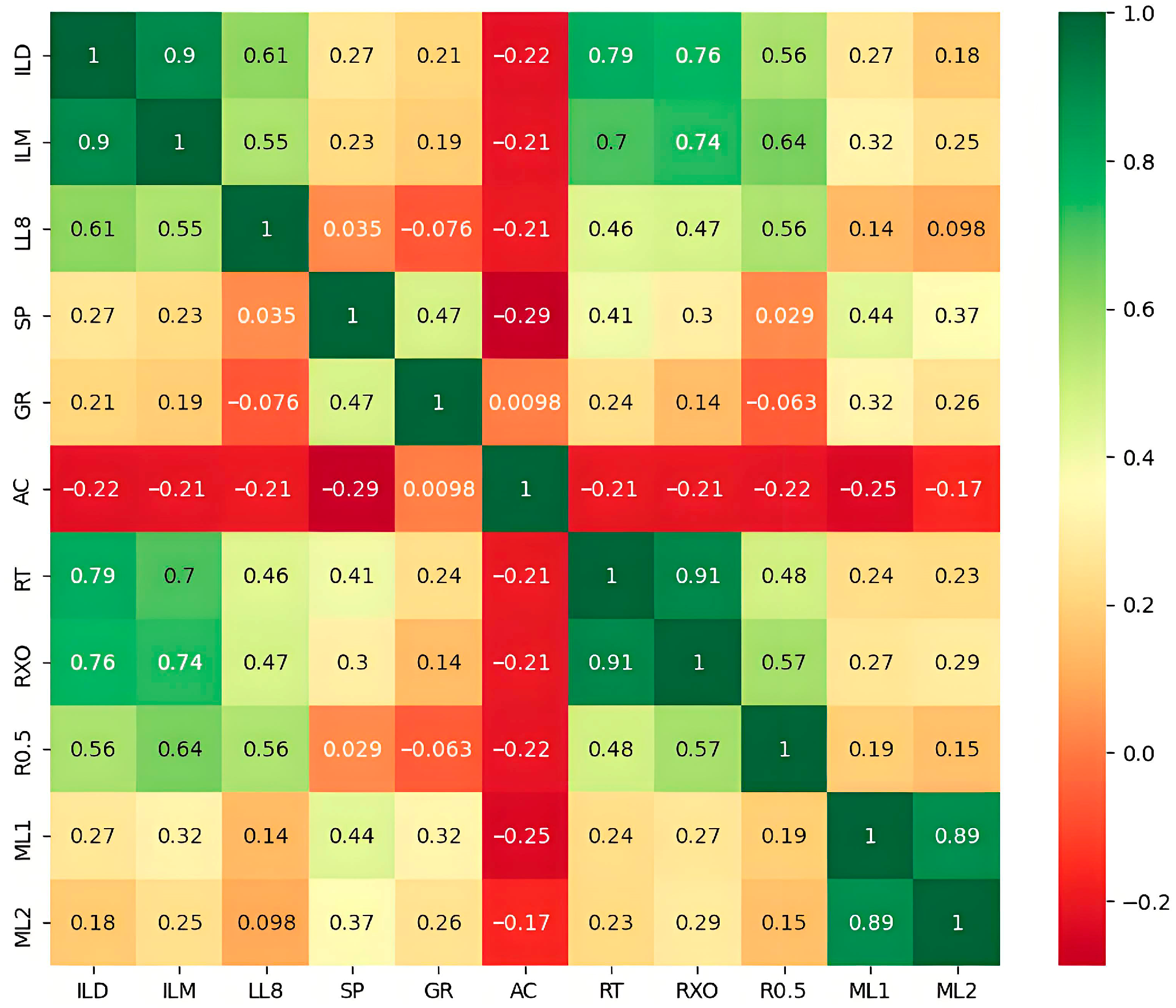
Figure 1. The correlation analysis of 11 kinds of characteristic parameters.
Processes 13 02775 g001
Figure 2. Workflow chart of porosity interpretation.
Processes 13 02775 g002
Figure 3. The 10-fold cross-validation of parameters C and γ in OVO SVMs.
Processes 13 02775 g003
Figure 4. The 10-fold cross-validation of parameters n_estimators and max_features in RF.
Processes 13 02775 g004
Figure 5. The 10-fold cross-validation of parameters n_estimators, max_depth, and learning_rate in XGBoost.
Processes 13 02775 g005
Figure 6. The 10-fold cross-validation of parameters iterations, depth, and learning_rate in CatBoost.
Processes 13 02775 g006
Figure 7. Training set accuracy, test set precision score, recall score, and F1 score of four models.
Processes 13 02775 g007
Figure 8. Confusion matrix plots on the test set of OVO SVM model.
Processes 13 02775 g008
Figure 9. Confusion matrix plots on the test set of RF model.
Processes 13 02775 g009
Figure 10. Confusion matrix plots on the test set of XGBoost model.
Processes 13 02775 g010
Figure 11. Confusion matrix plots on the test set of CatBoost model.
Processes 13 02775 g011
Figure 12. OVO SVM Taylor diagram.
Processes 13 02775 g012
Figure 13. RF Taylor diagram.
Processes 13 02775 g013
Figure 14. XGBoost Taylor diagram.
Processes 13 02775 g014
Figure 15. CatBoost Taylor diagram.
Processes 13 02775 g015
Figure 16. Feature importance analysis of RF model.
Processes 13 02775 g016
Table 1. Partially normalized data.
DepthILDILMLL8SPGRACRTRXOR0.5ML1ML2
2319.1250.1580970.311270.2600790.2687380.1530860.1987640.3004010.3526550.9497880.1046950.125684
2319.2500.1533990.2868220.2715050.2692310.1474430.1959260.3084350.366920.918250.0880320.085521
2319.3750.1477340.2589770.2603850.269970.1400370.1935240.3154760.3793130.8804610.1299920.127416
2319.5000.1403060.2286780.2219040.2709350.1350960.1933060.3212890.3892410.8372520.1906820.181097
2319.6250.1309390.1978860.1643520.2720880.1336870.1985460.3256850.3963810.7895910.2222650.220757
2319.7500.1205640.1705670.1044840.2733790.1403870.2109910.3285170.4006830.7384020.2519110.243474
2319.8750.1104040.1489110.0607930.2747780.1594360.2310790.3295760.4020970.6849510.2869810.268704
2320.0000.1007570.1326510.0364480.2762720.1802480.2566240.3285870.4006280.6309790.2865510.28751
2320.1250.0919390.1208130.0235160.2778380.2035290.2828250.3254420.396550.5759280.3467240.33769
2320.2500.0844410.1124620.0168240.2794120.23210.3053140.3196560.3893950.522010.3648090.384799
2320.3750.078150.1067030.0138120.2809560.2525580.3201620.3123120.3799630.4703740.1702080.206699
2320.5000.072920.1029170.0128770.282450.2656080.3258380.3037550.3685270.4215160.134190.121346
2320.6250.0689340.1004360.013150.283850.2730170.321690.294340.355230.3757670.1144270.103136
2320.7500.0658780.0987420.0141680.2851620.2719580.3074980.2842250.3402070.3336380.0994210.090418
Table 2. Results of the parameter optimization.
OVO SVM Optimal
Parameters
RF Optimal
Parameters
XGBoost Optimal
Parameters
CatBoost Optimal
Parameters
Cgamman_estimatorsmax_featuresn_estimatorsmax_depthlearning_rateiterationsdepthlearning_rate
20000.0014052050.15080.1
Table 3. STD, correlation, and RMSE of OVO SVM model.
ClassSTD_PredCorrelationRMSE
Class 10.0515940.8537790.046386
Class 20.2808060.9295770.106865
Class 30.4498750.9504490.146594
Class 40.3940540.9556540.120511
Class 50.0962260.9089630.046845
Class 60.0522040.9756840.017938
Class 70.0485000.9870330.008129
Table 4. STD, correlation, and RMSE of RF model.
ClassSTD_PredCorrelationRMSE
Class 10.0761980.9725550.019327
Class 20.2809920.9626240.077907
Class 30.4531230.9699930.114383
Class 40.3947440.9720660.095784
Class 50.0987800.9187950.044239
Class 60.0572420.9779190.014829
Class 70.0483820.9938520.005757
Table 5. STD, correlation, and RMSE of XGBoost model.
ClassSTD_PredCorrelationRMSE
Class 10.0440730.7814050.060956
Class 20.2215560.9326050.114025
Class 30.3579860.9526060.205588
Class 40.3130910.9582080.140226
Class 50.0665710.8479710.070348
Class 60.0265770.6725350.057876
Class 70.0365860.8196780.041750
Table 6. STD, correlation, and RMSE of CatBoost model.
ClassSTD_PredCorrelationRMSE
Class 10.0401240.8780110.050366
Class 20.2738690.9202210.113165
Class 30.4386190.9467220.152930
Class 40.3819070.9542570.122389
Class 50.0767520.8587720.060329
Class 60.0326950.7414800.046068
Class 70.0252010.7955440.033822
Disclaimer/Publisher’s Note: The statements, opinions and data contained in all publications are solely those of the individual author(s) and contributor(s) and not of MDPI and/or the editor(s). MDPI and/or the editor(s) disclaim responsibility for any injury to people or property resulting from any ideas, methods, instructions or products referred to in the content.