Abstract
To address the issues of reduced operational efficiency, shortened equipment lifespan, and significant safety hazards caused by bearing wear and blade cavitation in hydroelectric turbine generators due to prolonged high-load operation, this paper proposes a ResNet + self-attention-based acoustic fingerprint fault diagnosis algorithm for hydroelectric turbine generators. First, to address the issue of severe noise interference in acoustic signature signals, the ensemble empirical mode decomposition (EEMD) is employed to decompose the original signal into multiple intrinsic mode function (IMF) components. By calculating the correlation coefficients between each IMF component and the original signal, effective components are selected while noise components are removed to enhance the signal-to-noise ratio; Second, a fault identification network based on ResNet + self-attention fusion is constructed. The residual structure of ResNet is used to extract features from the acoustic signature signal, while the self-attention mechanism is introduced to focus the model on fault-sensitive regions, thereby enhancing feature representation capabilities. Finally, to address the challenge of model hyperparameter optimization, a Bayesian optimization algorithm is employed to accelerate model convergence and improve diagnostic performance. Experiments were conducted in the real working environment of a pumped-storage power station in Zhejiang Province, China. The results show that the algorithm significantly outperforms traditional methods in both single-fault and mixed-fault identification, achieving a fault identification accuracy rate of 99.4% on the test set. It maintains high accuracy even in real-world scenarios with superimposed noise and environmental sounds, fully validating its generalization capability and interference resistance, and providing effective technical support for the intelligent maintenance of hydroelectric generator units.
1. Introduction
As the core equipment of pumped-storage power plants, hydroelectric generator sets operate under high loads for extended periods, making them prone to faults such as bearing wear and blade cavitation. These faults can reduce operational efficiency, shorten equipment lifespan, and, in severe cases, cause shutdowns, leading to significant economic losses and safety hazards [1,2]. Therefore, timely and accurate diagnosis of the fault status of hydroelectric generator sets holds significant practical importance. The acoustic signals generated during the operation of hydroelectric generator sets contain valuable information reflecting the internal mechanical operating conditions of the equipment. When the operational status of the equipment changes, the corresponding acoustic signals undergo corresponding changes. Acoustic diagnosis technology [3,4,5] identifies faults by analyzing the acoustic signals generated during unit operation, without the need for disassembly or shutdown inspections, enabling early warning and diagnosis of faults without disrupting normal unit operation.
Extensive research has been conducted in the field of acoustic signature fault diagnosis for hydroelectric units [6,7,8]. Reference [9] utilizes acoustic signature information collected by non-contact microphone sensors to predict the remaining lifespan of rotating machinery, proposing a new method for selecting a subset of modulated spectral features using information theory methods. Reference [10] proposes an improved Mel-frequency cepstral coefficient feature extraction method for fault diagnosis of a gas-insulated switchgear (GIS) in power plants, and verifies that the proposed method can effectively improve the efficiency and reliability of online diagnosis of GIS. Reference [11] utilizes the significant changes in machine vibration frequency, vibration amplitude, and time-domain waveforms during faults to extract features from vibration signals to verify the corresponding fault types. Reference [12] characterizes the fault status of mechanical equipment by monitoring and analyzing the electrical signals generated by the target object. However, the fault feature information in the signals collected during the early stages of a fault is very weak, and the effectiveness of fault feature extraction using the electrical signal diagnosis method is generally poor. Reference [13] comprehensively analyzes vibration signals, electrical signals, and other monitoring parameters to achieve a more comprehensive diagnosis of the operating status of hydroelectric generator bearings; however, the cost of data acquisition is relatively high. However, the aforementioned literature relies on single feature thresholds or shallow machine learning models, making it difficult to effectively capture the complex relationship between the non-stationary characteristics of acoustic signals and faults, resulting in low fault diagnosis accuracy.
With the continuous development of deep learning, the diagnostic accuracy of hydroelectric generator sets has also improved [14,15]. Reference [16] proposed a method based on two-dimensional set local mean decomposition and optimized dynamic least squares support vector machines to rapidly and efficiently diagnose faults in anti-friction bearings. Reference [17] proposed a method for predicting bearing anomalies using LSTM-KLD, which utilizes divergence methods to uncover the distribution patterns of anomalous data and effectively extract data features. Reference [18] utilizes deep neural networks to extract sound signal features, achieving frame-level hierarchical classification with good classification results. Reference [19] employs a particle swarm optimization algorithm to enhance the extreme learning machine, combined with variational mode decomposition, to extract weak features from early-stage bearing fault monitoring data. Reference [20] employs an improved autoregressive integrated moving average (ARIMA) model to capture the temporal correlation and probability distribution of wind speed time series data, thereby constructing a time series-based prediction model, Reference [21] enhances the maintenance level of hydroelectric turbine units by extracting more sensitive IMF components from acoustic signals and training them using a convolutional neural network (CNN). Although these deep learning-based fault diagnosis methods can effectively identify common faults in hydroelectric generator units with the support of a large number of fault samples and different acoustic features, several key issues remain to be addressed in practical applications: (1) The complex network structure leads to a significant increase in computational load, resulting in degraded real-time system performance; (2) Traditional networks are constrained by gradient vanishing or explosion phenomena, making it difficult to extract effective features from high-dimensional data, and they are also prone to overfitting issues; (3) Existing defect diagnosis methods mostly only consider single defects in hydroelectric generator sets and do not consider acoustic pattern recognition issues when multiple defects occur simultaneously.
To address the issues of defect identification only considering single defects, high model complexity, and susceptibility to overfitting, this paper constructs a fault diagnosis model based on acoustic characteristics for hydroelectric generator sets using ResNet + self-attention. The main contributions of this paper are as follows:
- (1)
- To address the poor feature extraction capability of traditional diagnostic models, the network structure of the traditional residual network is optimized to enable deeper training for acoustic signature feature extraction, faster model convergence, and avoidance of gradient vanishing and explosion issues.
- (2)
- To address the varying contributions of different regions in acoustic signature signals to fault diagnosis, the self-attention mechanism is employed to enable the model to automatically focus on key features related to faults.
- (3)
- To address the issue of low diagnostic accuracy, we use Bayesian optimization algorithms to process high-dimensional hyperparameter spaces, accelerating model convergence and improving diagnostic performance.
- (4)
- We integrate the model into an edge computing platform and embed it into a hydroelectric generator acoustic monitoring system, validating the algorithm’s generalization capabilities in real-world noisy environments and providing a practical solution for intelligent maintenance of power equipment.
This paper first introduces the overall system structure and details the entire process of fault identification for hydroelectric generator sets based on acoustic signature signals. It then explains the acoustic signature noise reduction method for hydroelectric generator sets, first introducing the EEMD principle, then using correlation coefficient analysis to screen for effective signals, and finally providing the noise reduction process. It then focuses on analyzing the fault identification network, covering the self-attention mechanism, ResNet50 principle, fusion network architecture, and Bayesian optimization algorithm. Finally, through experiments in real-world environments, the algorithm’s effectiveness is validated from multiple aspects, including deployment, noise reduction, and diagnostic results.
2. System Architecture
The identification of acoustic faults in hydroelectric generator sets based on acoustic signals first involves using an acoustic signal acquisition device to collect sound signals from different fault states during the test operation of the hydroelectric generator set. This paper primarily analyzes bearing pitting, bearing wear, turbine blade cavitation, rotor imbalance, cooling system abnormalities, and mechanical loosening faults. The acoustic signature sequence signals obtained from different operating states are first subjected to noise reduction, i.e., the original signals are decomposed using EEMD to obtain different intrinsic modal IMF components, and the correlation coefficients between the different intrinsic modal IMF components and the original signals are calculated to screen out effective intrinsic modal components. The selected IMF components are then used as input feature datasets for the fault identification network. Using experimental operational acoustic signature signal sample data, the ResNet + self-attention network is trained. Finally, the trained hydroelectric turbine operational state recognition model is tested and validated using a test dataset to obtain the final fault identification results. The system architecture is shown in Figure 1.
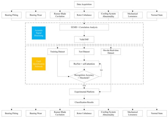
Figure 1.
System architecture diagram.
3. Noise Reduction of Voiceprint Signals
In actual engineering practice, the operating environment and conditions of hydroelectric generator sets are often complex, which can result in the collected acoustic fingerprint signals containing a significant amount of irrelevant noise. Acoustic fingerprint preprocessing first performs EEMD decomposition on the raw acoustic fingerprint signal x(t) to obtain several IMF components, and the correlation coefficients between the obtained IMF components and the original acoustic fingerprint signal are calculated. A screening threshold is set based on the comprehensive values of all correlation coefficients, and IMF components with correlation coefficients above the threshold are retained as valid signals, while those below the threshold are considered invalid noise and removed. The IMF components retained after correlation analysis are reconstructed into a new signal cj(t). The preprocessed signal better represents the acoustic signature signal characteristics of the hydroelectric turbine. The acoustic signature signal denoising principle flowchart is shown in Figure 2.
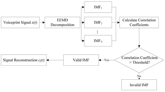
Figure 2.
Noise reduction of acoustic signal.
3.1. EEMD
EEMD is a process of adding white noise to the original signal and performing multiple EMD decompositions, which can effectively suppress modal aliasing problems and exhibit excellent performance when processing nonlinear and non-stationary signals. The process is as follows. Add a standard normal distributed white noise ni(t) to the original signal x(t):
where ni(t) represents the added Gaussian white noise, i is the added sequence, xi(t) is the signal data after adding Gaussian white noise, and i is the signal data sequence.
Perform EMD decomposition on the signal in (1) to obtain j modal components and one residual component:
where is the j-th modal component generated by EMD from xi(t) and one residual component, and ei(t) is the average trend of the signal. When the j-th residual component becomes a monotonic function and no further IMF components can be extracted, the screening process is terminated, and j is the selected number of modal components.
Repeat (1) and (2) N times to obtain the set of IMF components:
Perform ensemble averaging on the obtained IMF components to obtain the final components of EEMD:
where cj(t) is the j-th IMF component obtained from the EEMD.
In this paper, Nstd = 0.2 and NE = 100 are used as parameters for EEMD signal decomposition [22], where Nstd is the ratio of the standard deviation of the added noise to the standard deviation of the original signal, and NE is the number of times the signal is averaged.
3.2. Correlation Analysis
The correlation coefficient (CC) represents the degree of similarity between two different signals and can indicate the similarity between the IMF and the original signal. The closer the calculated correlation coefficient is to 1, the higher the similarity between the IMF signal and the original signal, and the better the IMF serves as an effective signal, effectively reflecting the characteristics and trends of the original signal. Its definition formula is as follows:
where Cov(X, Y) is the covariance between X and Y, and Var[·] represents the variance.
4. Fault Identification Network
The fault identification network trains the ResNet + self-attention network to classify faults using the denoised IMF signal as a dataset. To solve the model hyperparameter optimization problem, a Bayesian optimization mechanism is introduced to optimize the model’s hyperparameters. The workflow is shown in Figure 3.
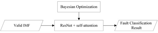
Figure 3.
Fault identification network workflow.
4.1. Self-Attention
In the task of acoustic fingerprint fault diagnosis for hydroelectric generator sets, acoustic fingerprint signals contain rich information, but the contribution of information from different regions to fault identification varies. The self-attention mechanism architecture is shown in Figure 4.
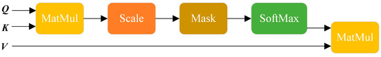
Figure 4.
Self-attention architecture.
For the input signal, a linear transformation is first applied to obtain the query matrix Q, key matrix K, and value matrix V. Then, the dot product of the query matrix Q and key matrix K is calculated and normalized using the SoftMax function to obtain the attention weight matrix, which describes the importance relationship between pixels in different regions of the feature map. Finally, the attention weight matrix is multiplied by the value matrix V to obtain the weighted feature representation:
By introducing the self-attention mechanism, the model can automatically learn the importance of different regions in the voiceprint signal, enabling it to more accurately capture key features related to faults and thereby improve the accuracy of fault diagnosis.
4.2. ResNet50
ResNet50 is a residual network with 50 layers, designed to address the issues of gradient vanishing or explosion that often arise during the training of deep neural networks. It enables the construction of deeper network models to learn more rich feature representations. It can automatically learn feature representations at different levels from acoustic feature maps, with lower-level residual blocks learning local features and higher-level blocks learning abstract global features, providing strong support for fault classification. The introduction of residual blocks and skip connections resolves gradient issues in deep network training, enabling the network to train deeper and learn complex features, thereby meeting the complexity and non-stationarity requirements of acoustic signals and ensuring good fault diagnosis performance under various operating environments and conditions.
4.3. ResNet + Self-Attention
Based on the analysis above, residual networks and attention mechanisms each have their unique advantages. Applying the attention mechanism globally can further enhance model performance. In this context, the three residual blocks at the end of the ResNet-50 model (one CRB and two IRBs) are replaced with three global self-attention blocks (GSABs). For shallow convolutions, applying self-attention to the extracted local features would result in high computational costs with low gains. In contrast, replacing the deep-layer, low-resolution, and high-channel feature maps with GSABs can effectively capture long-range dependencies. Moreover, the parameter count of these three layers accounts for only 10%, enabling an improvement in accuracy while controlling computational costs. In this module, the self-attention layer computes the global contextual features of the feature map input from the upper layer and performs weighted fusion of local features, thereby obtaining feature representations with higher discriminability and expressive power. Finally, the resulting outputs are fed into the subsequent pooling layer and fully connected layer to realize the integration of feature sets and decision-making, and the final classification results are obtained through the Softmax function. The network architecture is illustrated in Figure 5.
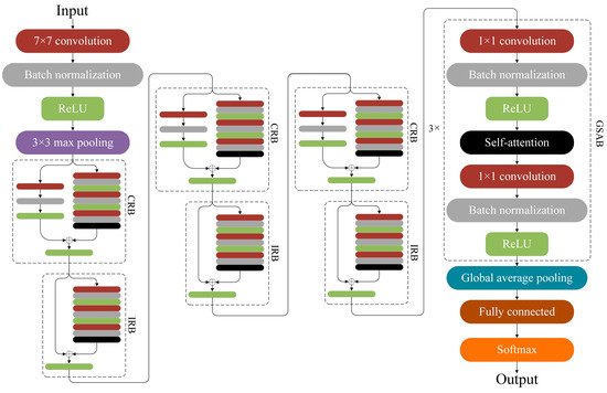
Figure 5.
ResNet + self-attention network architecture.
The specific operation process of the network is described as follows:
Let the input sample be x. Calculate the convolution of the convolution kernel and x to obtain the feature vector :
where and are the parameters to be trained.
Batch normalization (BN) is applied to to improve the training speed of the model. Let be an m × l matrix, and be the element in the i-th row and j-th column. The normalized result is expressed as:
where e is a small number to prevent the mean square deviation from being zero, is the element in the i-th row and j-th column, and γ and β are the parameters to be trained. At this point, the distribution of is adjusted to a standard normal distribution, which allows the input data to fall within the region where the activation function is most sensitive, thereby avoiding the vanishing gradient problem. However, this also leads to a decrease in the network’s expressive power, rendering the network’s depth meaningless. Therefore, it is necessary to perform the inverse operation on the transformed to enable the model to learn γ and β with optimal optimization effects.
Divide the normalized results into several non-overlapping segments, return the maximum value of each segment’s elements, and perform max pooling. This reduces the feature dimension and the number of parameters to be trained. The output of the max pooling layer is denoted as for the q × l matrix, and for the k-th row and j-th column elements of , denoted as:
where s is the length of the non-overlapping segment.
Thereafter, the abstract expression of pinp is extracted through multi-level residual units. The residual unit calculates the sum of the residual function and the input features, where the residual function is a nonlinear mapping composed of three convolutional layers :
where is the set of trainable parameters for the t-th residual unit. In this paper, t = 1, 2,…, 16. When t = 1, .
In IRB, the shortcut connection adds the features of two equal dimensions element-wise, i.e., an identity mapping. The output of the tth residual cell can be expressed as:
where is a multidimensional tensor. IRB does not introduce additional parameters or computational overhead to the model, offering significant advantages in practical applications.
In CRB, since the output channels of the convolutional layers are modified, the feature dimensions are unequal during addition, necessitating dimension matching in the shortcut connection (achieved via 1 × 1 convolution). This increases the network’s parameters but also enhances performance. The process can be represented as:
where and are the parameters to be trained.
After extracting device fault features from the 16-layer residual network, they are subjected to global average pooling (GAP) before being connected to a fully connected layer. GAP calculates the average value of each element in the feature matrix of each dimension to obtain a feature vector of length . Compared to directly connecting to the fully connected layer, this approach reduces network parameters and prevents overfitting.
Subsequently, the fully connected layer maps the features obtained from GAP to the sample’s label space, with the output denoted as:
where is the set of trainable parameters for the fully connected layer.
Finally, the Softmax function is used to calculate the probability distribution of in the label space. The probability of belonging to the s-th fault type is:
where is the set of parameters to be trained in the Softmax layer, and S is the total number of types. In this paper, S = 7. Finally, the category with the highest calculated probability is taken as the final classification result.
4.4. Bayesian Optimization
The Bayesian optimization algorithm is an algorithm for black-box function optimization problems, often used to optimize the hyperparameters of complex learning models. The algorithm estimates the objective function by continuously constructing a surrogate model, which is constructed by Gaussian Process Regression [23] (GPR), and the next parameter value is selected through a certain strategy to optimize the objective function. Figure 6 is the flowchart of the Bayesian optimization algorithm.
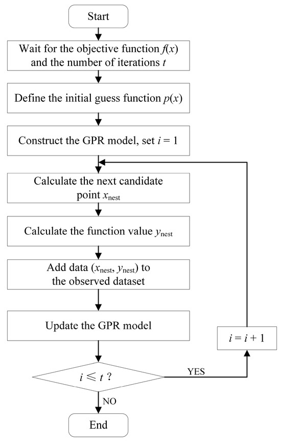
Figure 6.
Flowchart of Bayesian optimization algorithm.
In the process of hyperparameter optimization, the Bayesian optimization algorithm selects the next optimal hyperparameter point through a model-based method, avoiding calculation on all possible hyperparameter combinations, and finding the optimal hyperparameter point in relatively few iteration steps. The above advantages make Bayesian optimization especially suitable for practical problems where the computation is expensive or the objective function is difficult to optimize. The pseudocode of the algorithm is shown in Algorithm 1.
| Algorithm 1 Bayesian optimization algorithm |
| Input: objective function ; Search space: ; Initial observation set: , where , ; Maximum number of iterations: T; Stopping condition S; Output: optimal parameters ; Optimal value: Steps:
|
5. Experimental Results
5.1. Experiment Deployment
The experiment was carried out in the real working environment of a hybrid pumped storage power plant. The data acquisition system consisted of a Bruel & Kjær 4189 free-field microphone, an NI PXIe-4499 high-speed acquisition card, and an NVIDIA Jetson AGX Xavier edge computing platform. The data acquisition specifications are shown in Table 1.

Table 1.
Data acquisition specifications.
The sensor array is arranged at six key points such as the bearing seat, the frame, and the top cover of the unit to cover the radial/axial vibration-sensitive area. The composition of the data acquisition system is shown in Figure 7.
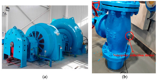
Figure 7.
Experimental platform. (a) Hydraulic turbine unit; (b) Voiceprint sensors.
The dataset construction is divided into three levels according to the degree of fault development, as shown in Table 2.
Table 2.
Classification criteria for fault severity.
Based on the fault severity grading criteria defined in Table 2, a library of acoustic pattern samples covering the full life cycle of the fault was constructed in this study. As shown in Table 3, six types of typical faults were collected according to three development stages: L1 (early), L2 (middle), and L3 (late). The sample size of L1–L3 levels for each type of fault is strictly controlled to within 85–86 groups, and the sample size of the normal state is 256 groups. These samples are divided into training set, validation set, and test set in the ratio of 7:3:1, and K-fold cross-validation is adopted for model training.
Table 3.
Distribution of classified dataset.
5.2. Hydroturbine Generator Set Voiceprint Noise Reduction Processing
The voiceprint signal from the Section 4.1 experimental equipment acquisition of datasets, including 20 samples of EEMD decomposition results, are shown in Figure 8.
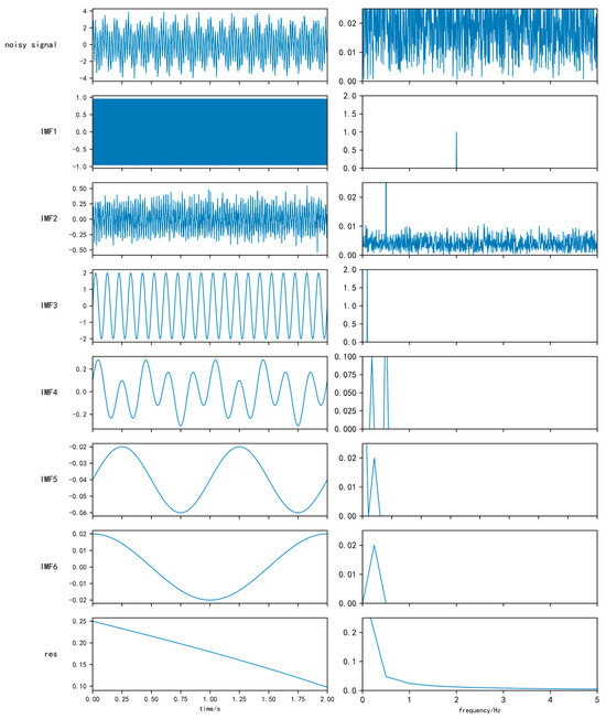
Figure 8.
EEMD decomposition and IMF spectrogram.
The EEMD diagrams in Figure 8 are on the left, and on the right are the corresponding spectra. EEMD will add a noise signal that is decomposed into six IMF components and a trend component, the IMF frequencies are arranged from high to low, each IMF contains certain frequency characteristics, and all the IMFs can decompose the signal before and after reorganization of the full spectrum diagram.
For all the IMF components with the original and the correlation analysis of the noise signal, the correlation coefficient was calculated; the results obtained are shown in Table 4.
Table 4.
Correlation coefficient calculation results.
The sequence numbers of IMF components with high correlation with the noise signal were 1, 3, and 4. The correlation coefficients calculated for the trend components of 5, 6, and Res in the remaining IMFs were very small, which could be identified as low-frequency interference noise. The IMF2 correlation coefficient value is smaller than those of IMF components 1 and 4. Combined with the Figure 2 spectrum, it can be concluded that IMF2 for the noise signal of high-frequency interference and noise will retain the serial numbers 1, 3, 4 of the IMF component after restructuring for the new denoising signal.
5.3. The Bayesian Fault Diagnosis Results After Optimization
In this paper, Bayesian optimization is used to optimize the initial learn rate of a single hyperparameter for 30 times in the range of (1 × 10⁻⁵, 0.1). Kullback–Leibler (KL) divergence is used in the process of model training and validation. In the process of model training and validation, KL divergence is used as the loss function, and the optimization process is plotted as a curve, and the abscissas are logarithmic coordinates. The accuracy comparison under different initial learning rates is shown in Figure 9, and the loss value comparison under different initial learning rates is shown in Figure 10.
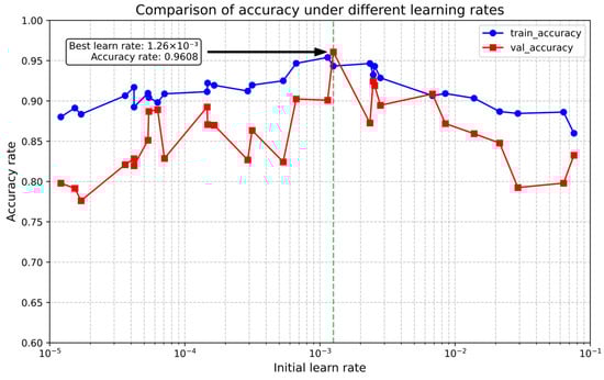
Figure 9.
Comparison of accuracy under different initial learning rates.
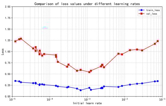
Figure 10.
Comparison of loss values with different initial learning rates.
As shown in Figure 9, the accuracy does not change monotonically with the learning rate; instead, it reaches a peak at a specific learning rate (e.g., 0.00126). This indicates that an appropriate learning rate can significantly enhance the model’s fitting ability. During the Bayesian optimization process, when the initial learning rate is set to 0.00126, the validation set accuracy reaches the maximum of 96.08%. Figure 10 demonstrates that the loss value first decreases and then increases with the increase in the learning rate, with the minimum loss achieved under the optimal learning rate, where the validation loss is 0.67.
The ResNet + self-attention network model trained under this condition was exported and tested using the test set data. Figure 11 presents the confusion matrix derived from the test results. This fault identification confusion matrix shows that the model exhibits excellent classification performance for faults: the test accuracy of the model trained with the optimized learning rate reaches 99.4%, with both precision and recall for all categories being ≥0.99, and the average F1-score reaching 0.997. Specifically, categories 1, 2, 4, and 7 achieve 100% precision and recall; only categories 3, 5, and 6 have 1–2 instances of misclassification into adjacent categories (e.g., category 5 → 6, category 6 → 7). However, the overall cross-confusion rate is extremely low, indicating that the model possesses extremely high recognition stability and accuracy for both single and mixed faults, thus verifying the effectiveness of the Bayesian optimization algorithm.
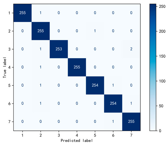
Figure 11.
Confusion matrix diagram for fault identification.
5.4. Single Fault and Mixed Fault Recognition Results
Figure 12a shows the comparison between the actual and simulated normal signals, Figure 12b shows the comparison between the actual and simulated single faults (bearing pitting), Figure 12c shows the comparison between the actual and simulated mixed faults (bearing wear + blade cavitation), and Figure 12d is the comprehensive comparison. In the normal signal spectrum, both the actual and simulated signals are dominated by the fundamental frequency. The actual signal has slight spurs due to environmental noise, which confirms the stability of the fundamental frequency dominance in normal signals. In the single fault spectrum, the simulated signal clearly contains impact harmonics. Although the actual signal has spurs affected by noise, the core frequencies are consistent, which verifies the necessity of EEMD denoising for retaining fault features. In the mixed fault spectrum, the simulated signal shows the superposition of characteristic frequencies at 1.5 kHz, 8 kHz, and 12 kHz, and the core frequencies of the actual signal are consistent with it, reflecting the algorithm’s ability to analyze complex spectra. The comprehensive comparison chart intuitively shows significant spectral differences between different states, and the core frequencies of the actual and simulated signals are consistent, with only the actual signal affected by noise. This confirms that the algorithm still has high diagnostic accuracy in actual scenarios through denoising, feature focusing, and Bayesian optimization.
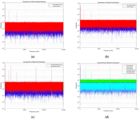
Figure 12.
Spectra of single faults and mixed faults. (a) Comparison of normal signal spectra; (b) Comparison of single fault spectra; (c) Comparison of mixed fault spectra; (d) Comprehensive spectral comparison.
As can be seen from the data in Table 5, in the condition of a single fault test, model accuracy is as high as 99.80%. The results show that when the hydro-generator units experience only a single type of failure, the algorithm can very accurately identify the fault type. In the mixed fault test state, the accuracy of the model reaches 98.63%. Although the accuracy of the model is slightly decreased compared with that of single fault recognition, it still remains at a high level, showing that in practice, when the hydroelectric generating set experiences a variety of problems at the same time, the algorithm can effectively extract the key features from the complex voiceprint signal and accurately identify mixed fault types, showing that the algorithm is capable of dealing with complex fault situations of stability and reliability.
Table 5.
Single fault and mixed fault identification results.
5.5. Test Results Under the Sound Environment with Added Noise
Table 6 shows the algorithm test results under added noise and environmental sound. The data in the table shows that, under the conditions of the normal state and the normal state after adding the noise signal, the algorithm accuracy reached 100%, showing that the algorithm, in the normal state and in the normal state after adding the noise signal, can maintain better recognition ability and will not show much misjudgment; the algorithm has certain anti-interference ability. In the fault state, for all kinds of fault signals, such as bearing pitting, bearing wear, runner blade cavitation, rotor unbalance, cooling system anomality, and mechanical looseness fault, whether it is a simple fault signal or a fault signal with noise, the algorithm achieves 1500/1500 recognition results, and the accuracy rate is also 100%. It is fully proven that the proposed algorithm can effectively extract fault features in the face of an actual complex acoustic environment, and accurately identify various fault types without the interference of noise and environmental sound.
Table 6.
Test results under additive noise and ambient sound.
5.6. Comparison of Algorithm Performance
Table 7 presents a performance comparison between the algorithm proposed in this paper and LSTM-KLD [17], Modified-ARIMA [20], CNN [21], ResNet50, and LSTM under four different scenarios: fault identification without voiceprint denoising, fault identification after voiceprint denoising, datasets with added noise, and datasets containing mixed faults.
Table 7.
Comparison of algorithm performance.
- (1)
- The fault identification of silent grain noise reduction
The accuracy of the proposed algorithm reaches 88.12%, which is higher than that of the other five algorithms. Among them, ResNet50 (84.22%) and Modified-ARIMA (85.44%) perform sub-optimally but are both lower than the proposed algorithm. This indicates that without denoising the voiceprint signals, the proposed algorithm can more effectively extract fault features from the original voiceprint signals and has stronger fault recognition capability. In terms of time consumption, the proposed algorithm takes 10.01 s, which is significantly faster than LSTM (25.55 s) and ResNet50 (22.15 s), demonstrating that the proposed algorithm has obvious advantages in computational efficiency and can complete the fault identification task in a shorter time.
- (2)
- After a voiceprint noise fault recognition
The accuracy of the proposed algorithm reaches 100.0%, which is significantly higher than CNN (96.67%) and Modified-ARIMA (95.15%). This shows that after voiceprint denoising, the proposed algorithm can give full play to its advantages, capture fault features more accurately, and achieve completely accurate fault identification. In terms of time consumption, the proposed algorithm takes 4.02 s, which is much lower than ResNet50 (18.22 s) and LSTM (12.74 s), further reflecting the superiority of the proposed algorithm in computational efficiency, which can quickly complete fault diagnosis while ensuring high accuracy.
- (3)
- Increasing noise in the dataset
The accuracy of the proposed algorithm is 98.24%, higher than that of CNN (94.54%) and Modified-ARIMA (92.12%). This indicates that when noise interference is added to the dataset, the proposed algorithm has strong anti-interference ability and can still accurately identify faults in complex noise environments. In terms of time consumption, the proposed algorithm takes 6.03 s, significantly faster than ResNet50 (17.55 s) and LSTM (13.69 s), indicating that when processing noisy datasets, the proposed algorithm can not only maintain high accuracy but also complete fault diagnosis at a faster speed, showing good real-time performance.
- (4)
- Dataset containing mixed fault condition
The accuracy of the proposed algorithm is 98.22%, which is significantly higher than other algorithms (the highest for CNN is 91.52%). This indicates that when the dataset contains a mixture of multiple fault types, the proposed algorithm can effectively distinguish different fault features from complex voiceprint signals and achieve accurate identification of mixed faults. In terms of time consumption, the proposed algorithm takes 6.83 s, much faster than ResNet50 (19.52 s) and LSTM (18.11 s), indicating that the proposed algorithm also has efficient computing capability when processing mixed faults and can provide accurate diagnosis results in a shorter time.
6. Conclusions
The proposed voiceprint fault diagnosis algorithm for hydroturbine units based on ResNet + self-attention significantly improves the accuracy of fault diagnosis by combining a residual network and self-attention mechanism. At the same time, through the Bayesian optimization algorithm processing high-dimensional parameter space, it accelerates the model convergence, and the algorithm is verified in a noisy environment. The experimental results show that the proposed algorithm achieves excellent performance in single fault and mixed fault recognition, and the accuracy is much higher than that of traditional methods. Especially in the actual application scenarios of superimposed noise and environmental sound, the proposed algorithm can still maintain a high diagnostic accuracy, which fully proves its effectiveness and generalization ability in practical applications. In the future, the algorithm structure will be further optimized to improve the real-time performance of the model, and its application potential in the fault diagnosis of other mechanical equipment will be explored.
Author Contributions
Conceptualisation, W.W., J.X.; methodology, X.L. and K.T.; software, J.W. and Y.Z.; validation, Y.L.; formal analysis, Y.L.; investigation, K.S. and X.M.; data curation, Y.L.; writing—original draft preparation, Y.L.; writing—review and editing, Y.L.; visualisation, Y.L.; supervision, W.W., J.X. and Y.L. All authors have read and agreed to the published version of the manuscript.
Funding
This research was funded by Zhejiang Huadian Quzhou Wuxijiang 298MW Hybrid Pumped Storage Power Station Project (2205-330000-04-01-177202).
Data Availability Statement
The original contributions presented in this study are included in the article. Further inquiries can be directed to the corresponding author.
Conflicts of Interest
Authors Wei Wang, Xin Li, Kang Tong, Kailun Shi and Xin Mao were employed by the Zhejiang Huadian Wuxijiang Hybrid Pumped Storage Power Generation Co., Ltd. Authors Jiaxiang Xu, Junxue Wang and Yunfeng Zhang were employed by Three Gorges High-Tech Information Technology Co., Ltd. The remaining author declares that the research was conducted in the absence of any commercial or financial relationships that could be construed as a potential conflict of interest.
References
- Liu, Y.; Wu, L.; Yang, Y.; Chen, Y.; Baldick, R.; Bo, R. Secured Reserve Scheduling of Pumped-Storage Hydropower Plants in ISO Day-Ahead Market. IEEE Trans. Power Syst. 2021, 36, 5722–5733. [Google Scholar] [CrossRef]
- Kumari, R.; Prabhakaran, K.K.; Desingu, K.; Chelliah, T.R.; Sarma, S.V.A. Improved Hydroturbine Control and Future Prospects of Variable Speed Hydropower Plant. IEEE Trans. Ind. Appl. 2021, 57, 941–952. [Google Scholar] [CrossRef]
- Zhang, K.; Lu, H.; Han, S.; Zhao, X. A Novel Fault Diagnosis Method for Power Transformers Based on Voiceprint Recognition Considering Multitype Noises. IEEE Trans. Instrum. Meas. 2025, 74, 1. [Google Scholar] [CrossRef]
- Yu, Z.; Wei, Y.; Niu, B.; Zhang, X. Automatic Condition Monitoring and Fault Diagnosis System for Power Transformers Based on Voiceprint Recognition. IEEE Trans. Instrum. Meas. 2024, 73, 9600411. [Google Scholar] [CrossRef]
- Zhao, C.; Zhang, L.; Zhong, M. Fault diagnosis for wind turbine gearbox based on recurrent convolutional generative adversarial network. J. Shandong Univ. Sci. Technol. (Nat. Sci.) 2024, 43, 109–118. [Google Scholar]
- He, X.; Pan, R.; Hao, Z.; Lin, Z.; Bai, T.; Peng, J. Research on Small Sample Voiceprint Recognition Method for Hydroelectric Units Based on Deep Prototype Network. In Proceedings of the 2023 IEEE 11th Joint International Information Technology and Artificial Intelligence Conference, Chongqing, China, 8–10 December 2023; pp. 433–436. [Google Scholar]
- Lv, Y.; Xu, L.; Yin, C.; Lin, Y.; Lu, C.; Liu, T.; Dai, C. Overview of Abnormal Sound Detection for Hydroelectric Generating Units. In Proceedings of the 2023 7th International Conference on Electrical, Mechanical and Computer Engineering, Xi’an, China, 20–22 October 2023; pp. 597–604. [Google Scholar]
- Rong, Y.; Fang, Y.; Tian, P.; Cheng, J. Voiceprint recognition based on knowledge distillation and ResNet. J. Chongqing Univ. (Nat. Sci. Ed.) 2023, 46, 113–124. [Google Scholar]
- Scanlon, P.; Kavanagh, D.F.; Boland, F.M. Residual Life Prediction of Rotating Machines Using Acoustic Noise Signals. IEEE Trans. Instrum. Meas. 2013, 62, 95–108. [Google Scholar] [CrossRef]
- Honggang, C.; Mingyue, X.; Chenzhao, F.; Renjie, S.; Zhe, L. Mechanical Fault Diagnosis of GIS Based on MFCCs of Sound Signals. In Proceedings of the 2020 5th Asia Conference on Power and Electrical Engineering, Chengdu, China, 4–7 June 2020; pp. 1487–1491. [Google Scholar]
- Zhang, F.; Guo, J.; Yuan, F.; Shi, Y.; Li, Z. Research on Denoising Method for Hydroelectric Unit Vibration Signal Based on ICEEMDAN–PE–SVD. Sensors 2023, 23, 6368. [Google Scholar] [CrossRef] [PubMed]
- Guan, B.; Bao, X.; Qiu, H.; Yang, D. Enhancing bearing fault diagnosis using motor current signals: A novel approach combining time shifting and CausalConvNets. Measurement 2024, 226, 114049. [Google Scholar] [CrossRef]
- Zhang, Y.; Yang, K. Fault Diagnosis of Submersible Motor on Offshore Platform Based on Multi-Signal Fusion. Energies 2022, 15, 756. [Google Scholar] [CrossRef]
- Radicioni, L.; Giorgi, V.; Benedetti, L.; Bono, F.M.; Pagani, S.; Cinquemani, S.; Belloli, M. On the performance of data-driven dynamic models for temperature compensation on bridge monitoring data. J. Civ. Struct. Health Monit. 2025, 15, 1957–1972. [Google Scholar] [CrossRef]
- Mao, P.; Zhang, Y.; Li, W.; Shi, Z. Research on Voiceprint Recognition Method of Hydropower Unit Online-State Based on Mel-Spectrum and CNN. In Proceedings of the 2024 IEEE 8th Conference on Energy Internet and Energy System Integration, Shenyang, China, 29 November–2 December 2024; pp. 7–11. [Google Scholar]
- Xiong, Z.; Han, C.; Zhang, G. Fault diagnosis of anti-friction bearings based on Bi-dimensional ensemble local mean decomposition and optimized dynamic least square support vector machine. Sci. Rep. 2023, 13, 17784. [Google Scholar] [CrossRef] [PubMed]
- Wu, Y.; Ma, X. A hybrid LSTM-KLD approach to condition monitoring of operational wind turbines. Renew. Energy 2022, 181, 554–566. [Google Scholar] [CrossRef]
- Heigold, G.; Moreno, I.; Bengio, S.; Shazeer, N. End-to-end text-dependent speaker verification. In Proceedings of the 2016 IEEE International Conference on Acoustics, Speech and Signal Processing, Shanghai, China, 20–25 March 2016; pp. 5115–5119. [Google Scholar]
- Li, K.; Su, L.; Wu, J.; Wang, H.; Chen, P. A Rolling Bearing Fault Diagnosis Method Based on Variational Mode Decomposition and an Improved Kernel Extreme Learning Machine. Appl. Sci. 2017, 7, 1004. [Google Scholar] [CrossRef]
- Yunus, K.; Thiringer, T.; Chen, P. ARIMA-Based Frequency-Decomposed Modeling of Wind Speed Time Series. IEEE Trans. Power Syst. 2016, 31, 2546–2556. [Google Scholar] [CrossRef]
- Xiao, B.; Zeng, Y.; Hu, W.; Cheng, Y. Feature Extraction of Flow Sediment Content of Hydropower Unit Based on Voiceprint Signal. Energies 2024, 17, 1041. [Google Scholar] [CrossRef]
- Wu, Z.; Huang, N.E. Ensemble Empirical Mode Decomposition: A Noise-Assisted Data Analysis Method. Adv. Adapt. Data Anal. 2009, 1, 1–41. [Google Scholar] [CrossRef]
- Duan, J.; Tang, Q.; Ma, J.; Yao, W. Operational Status Evaluation of Smart Electricity Meters Using Gaussian Process Regression with Optimized-ARD Kernel. IEEE Trans. Ind. Inform. 2024, 20, 1272–1282. [Google Scholar] [CrossRef]
Disclaimer/Publisher’s Note: The statements, opinions and data contained in all publications are solely those of the individual author(s) and contributor(s) and not of MDPI and/or the editor(s). MDPI and/or the editor(s) disclaim responsibility for any injury to people or property resulting from any ideas, methods, instructions or products referred to in the content. |
© 2025 by the authors. Licensee MDPI, Basel, Switzerland. This article is an open access article distributed under the terms and conditions of the Creative Commons Attribution (CC BY) license (https://creativecommons.org/licenses/by/4.0/).