Abstract
Machine predictive maintenance plays a critical role in reducing unplanned downtime, lowering maintenance costs, and improving operational reliability by enabling the early detection and classification of potential failures. Artificial intelligence (AI) enhances these capabilities through advanced algorithms that can analyze complex sensor data with high accuracy and adaptability. This study introduces an explainable AI framework for failure detection and classification using symbolic expressions (SEs) derived from a genetic programming symbolic classifier (GPSC). Due to the imbalanced nature and wide variable ranges in the original dataset, we applied scaling/normalization and oversampling techniques to generate multiple balanced dataset variations. Each variation was used to train the GPSC with five-fold cross-validation, and optimal hyperparameters were selected using a Random Hyperparameter Value Search (RHVS) method. However, as the initial Threshold-Based Voting Ensembles (TBVEs) built from SEs did not achieve a satisfactory performance for all classes, a meta-dataset was developed from the outputs of the obtained SEs. For each class, a meta-dataset was preprocessed, balanced, and used to train a Random Forest Classifier (RFC) with hyperparameter tuning via RandomizedSearchCV. For each class, a TBVE was then constructed from the saved RFC models. The resulting ensemble demonstrated a near-perfect performance for failure detection and classification in most classes (0, 1, 3, and 5), although Classes 2 and 4 achieved a lower performance, which could be attributed to an extremely low number of samples and a hard-to-detect type of failure. Overall, the proposed method presents a robust and explainable AI solution for predictive maintenance, combining symbolic learning with ensemble-based meta-modeling.
1. Introduction
Predictive maintenance (PdM) is a transformative approach in industrial settings, allowing for the proactive monitoring and maintenance of machinery before failures occur [1]. Unlike traditional preventive maintenance, which operates on fixed schedules, predictive maintenance focuses on identifying patterns in operational data to predict when a machine is likely to fail [2]. This helps organizations avoid costly unplanned downtime, extend equipment lifespan, and reduce unnecessary maintenance costs [3]. Machine predictive maintenance classification plays a crucial role in this domain by leveraging historical and real-time data to classify machine health into categories such as “normal,” “warning,” or “failure imminent.” This classification is essential for decision making, enabling maintenance teams to prioritize actions and allocate resources efficiently.
PdM has become increasingly critical due to the rising complexity, scale, and operational cost sensitivity of modern industrial systems. Unplanned downtime imposes a significant economic burden—according to the Uptime Institute [4], unexpected outages cost businesses an average of USD 260,000 per hour, with high-volume manufacturing plants losing over USD 2 million per hour in halted production. A study by Deloitte [5] estimates that predictive maintenance can reduce equipment breakdowns by up to 70%, lower maintenance costs by 25%, and cut downtime by 35%.
In the energy sector, predictive models have been successfully deployed in wind farms and photovoltaic power plants to detect anomalies early, thereby increasing energy yield and extending the life of critical components [6]. Similarly, in aviation, predictive maintenance algorithms are applied to identify faults in engines and flight systems well before they lead to failure, improving both safety and fleet availability [7].
Given the high stakes involved—both financial and safety-related—there is an urgent need for robust, accurate, and explainable AI-based predictive maintenance solutions that can be trusted and understood by engineers, regulators, and stakeholders alike.
Machine learning (ML) has emerged as a powerful tool for achieving predictive maintenance classification [8]. Modern machinery generates vast amounts of sensor data, including vibration, temperature, pressure, and acoustic signals, which can be analyzed using ML algorithms. By training classification models on labeled datasets, ML systems can learn to recognize subtle patterns or anomalies that precede failure. Techniques such as decision trees, Support Vector Machines (SVMs), and neural networks allow for accurate predictions even in complex systems. Moreover, advanced algorithms can handle high-dimensional and noisy data, making it possible to detect early signs of degradation that might go unnoticed through manual inspections.
The importance of machine predictive maintenance classification extends beyond operational efficiency. In industries such as manufacturing, transportation, energy, and healthcare, critical systems must operate reliably. Predictive maintenance helps avoid catastrophic failures that could jeopardize safety or incur massive financial losses. For example, in wind farms or photovoltaic power plants, predictive classification models can monitor turbines or solar panels for faults, ensuring continuous energy production and reducing downtime. In aviation, predictive models enhance safety by identifying potential failures in engines or critical components well before they happen.
The integration of machine learning into predictive maintenance also enables scalability and adaptability. With the advent of IoT (Internet of Things) devices and edge computing, real-time data from connected machines can be processed locally or in the cloud, making predictions available instantaneously. Furthermore, ML models can adapt to evolving operating conditions by continuously learning from new data. As a result, predictive maintenance systems become smarter and more accurate over time.
The authors of [9] used Support Vector Machines (SVMs), a Decision Tree Classifier, k-nearest neighbors, a Random Forrest Classifier (RFC), and an Artificial Neural Network to detect industrial machine failure from the small predictive maintenance dataset. In [10], a deep auto-encoder (DAE) was used for machine tools fault detection. The highest accuracy achieved with the DAE is 98.1%. The bearing fault detection using an ANN, radial basis function (RBF) network, and probabilistic neural network (PNN) was performed in [11]. All these networks were also combined with a genetic algorithm to find optimal architecture using whichever highest classification performance could be achieved. The highest classification performance was achieved with GPA + ANN and GA + RBF of 100%. Power Transmission Line fault detection was investigated in [12] using a feed-forward ANN. The detection achieved using an ANN was 100%. The intelligent model that integrates a combination of a gated residual neural network (GRN) and a multi-head self-attention mechanism (MHSA) was used in [13] for photovoltaic (PV) arrays fault detection. The proposed model achieved 99.71% accuracy. The authors of [14] used convolutional neural networks (CNNs) that used vibration measurements as input data acquired in a laboratory environment from the ball bearings of a motor for predictive maintenance. The highest results on the experimental data achieved 100% accuracy. In [15], the authors used sensor data to predict aircraft engine failure within a predetermined number of cycles using Long Short-Term Memory (LSTM), Recurrent Neural Networks (RNNs), a Gated Recurrent Unit (GRU) RFC, KNN, Naive Bayes (NB), and Gradient Boosting (GB). The highest accuracy of 97.18% was achieved with a GRU. The authors of [16] used various ML algorithms for predictive maintenance, and the highest accuracy of 99.91% achieved was with an Ada Boost Classifier (ABC).
In Table 1, the summary of the results achieved in other research papers is listed.

Table 1.
The summary of the results achieved in other research papers.
In the context of predictive maintenance, interpretability is not just a desirable property—it is often essential. Many conventional ML and deep learning (DL) models, such as ANNs and DAEs, are considered black-box models (Table 1). While these models can achieve a high predictive performance, they provide little insight into why a certain prediction was made, which is a critical limitation in high-stakes industrial settings. For example, when a model flags a machine component as likely to fail, maintenance engineers need to understand the reasoning behind this decision in order to validate the alert, diagnose the root cause, and determine the appropriate intervention. Without transparency, such systems may not be trusted or accepted in production environments—particularly in safety-critical industries like aviation, manufacturing, or energy, where decisions must be explainable and auditable.
Moreover, regulatory compliance and risk management frameworks often require transparent decision making, especially in the context of equipment health monitoring. Interpretability also enables human-in-the-loop systems, where experts can combine model insights with domain knowledge to improve system reliability. Unlike black-box models, symbolic expressions generated by genetic programming symbolic classifiers (GPSCs) are explicit mathematical formulas, which allow practitioners to understand and audit how specific input features contribute to failure detection or classification. This level of transparency enables faster troubleshooting, model validation, and knowledge transfer, making explainable models more practical and trustworthy for long-term predictive maintenance deployments.
Thus, our proposed method addresses a critical gap by offering a robust, accurate, and inherently interpretable AI solution for predictive maintenance—unlike many prior studies that rely on opaque ML systems with limited real-world applicability in sensitive or regulated environments.
The novelty of this paper is the development of the explainable model in the form of symbolic expressions (SEs) that are used for machine fault detection and classification. The SEs will be obtained using a GPSC that will be trained on the publicly available dataset. The dataset target variable contains multiple classes; however, the GPSC can not handle multi-class problems, so the one-versus-rest method will be applied, and by doing so, from the initial dataset, multiple datasets will be generated, where each will contain a different class as the target variable. The scaling/normalization techniques and different oversampling techniques will be applied to create scaled/normalized balanced dataset variations, and on each GPSC, they will be trained. This process is developed to obtain a large number of SEs. Since GPSCs have a large number of hyperparameters, finding the optimal combination of these hyperparameters can be a great challenge. To overcome this challenge, the random hyperparameter values search method (RHVS) was developed and applied that will randomly select the values of each hyperparameter before each GPSC training. The goal is to find, using RHVS, the optimal combination of GPSC hyperparameters as quick as possible to obtain SEs that can achieve a high classification performance. The GPSC is trained using five-fold cross-validation (5FCV), meaning it is trained five times, each on a different training subset. After each fold, a symbolic expression (SE) is generated. This results in five symbolic expressions per dataset variation—referred to as 5SEs. These expressions increase the diversity and number of high-performing SEs. To further improve performance and robustness, we aggregate the outputs of multiple SEs using a Threshold-Based Voting Ensemble (TBVE), which selects class predictions based on whether the number of SEs voting for a class exceeds a predefined threshold.
In case the TBVE based on the SEs obtained from the GPSC will fail, the backup strategy is to obtain the meta-dataset from these SEs using the initial imbalance dataset and then subject the meta-dataset to preprocessing and oversampling techniques. Each dataset will be used to train the Random Forest Classifier (RFC) with the RandomizedSearchCV, and the best RFC models will be saved. The saved RFC models will be combined into TBVEs for each class and evaluated on the initial imbalanced dataset.
Based on the overview of other research papers and the proposed novelty, the following questions arise:
- Is it possible to obtain SEs using the GPSC for machine failure detection/classification with a high classification performance?
- Is it possible to generate scaled/normalized balanced dataset variations using scaling/normalization and oversampling techniques, and is there any influence of the classification performance on the obtained SEs?
- Is it possible to find the optimal combination of GPSC hyperparameters with the RHVS method using whichever generated SEs achieved the highest classification performance?
- Is it possible to obtain a robust set of SEs when the GPSC is trained using 5FCV?
- Is it possible to improve the classification performance by developing the TBVE and adjusting the threshold values?
- If the TBVE based on SEs fails, is it possible to create a meta-dataset based on the SEs outputs, then use this meta-dataset and subject it to various preprocessing + oversampling techniques and train the RFC on each balanced dataset variation, and after that combine the best RFC models in the TBVE for each class and achieve the highest classification performance?
The outline of this paper consists of the following sections: Materials and Methods, Results, Discussion, and Conclusions. Section 2 contains the research methodology, a description of the dataset with detailed statistical analysis, a description of preprocessing and oversampling techniques, a genetic programming symbolic classifier with the random hyperparameters values search method, evaluation metric techniques, the training testing procedure, and Threshold-Based Voting Ensembles. Section 3 contains the analysis of the results obtained on balanced dataset variations and the analysis of the results obtained on the TBVE. Section 4 contains the discussion about the results obtained with the proposed research methodology. Section 5 contains basic information about the proposed research methodology, the answers to the hypotheses proposed in this section, the advantages and disadvantages of the proposed research methodology, and finally directions for potential improvement, i.e., directions for future work. Additionally, the appendix section provides information about the mathematical functions that had to be modified to avoid early terminations of the GPSC due to imaginary or non-number values and where to download all obtained SEs and how to use them.
2. Materials and Methods
2.1. Research Methodology
The research methodology used in this paper is graphically shown in Figure 1.
Figure 1.
The graphical illustration of research methodology.
The research methodology shown in Figure 1 consists of the following steps:
- Step 1—Perform the initial dataset statistical analysis and create different variations of the dataset using data scaling/normalization techniques and oversampling techniques, thus creating multiple variations of the initial datasets.
- Step 2—Train the GPSC using the 5-fold cross-validation process and the RHVS method to obtain a set of SEs with a high classification performance on each balanced dataset variation. The RHVS method is used to find the optimal combination of GPSC hyperparameter values using whichever GPSC generates SEs with the highest classification performance on each balanced dataset variation.
- Step 3—Perform the detailed investigation of the best sets of SEs and select only those that have a classification performance higher than 0.95.
- Step 4—Create the Threshold-Based Voting Ensembles (TBVEs) and adjust the threshold value to see if classification performance could be improved when compared to single SEs. If the TBVE based on SEs fails, create the dataset of SEs outputs, apply the preprocessing + oversampling techniques to create balanced dataset variations, and train the RFC using 5FCV and the random hyperparameter search. After the RFCs are trained, create the TBVE based on the RFC and find the optimal threshold value using whichever highest classification performance is achieved.
2.2. Dataset Description and Statistical Analysis
The dataset used in this investigation is a publicly available dataset (see the Data Availability Statement). The dataset is a synthetic dataset that reflects real predictive maintenance encountered in the industry. The dataset consists of 10,000 data samples and 14 variables (features). These variables are as follows:
- 1.
- UID—Unique identifier ranging from 1 to 100,000.
- 2.
- Product ID—The product unique identifier.
- 3.
- Air temperature [K]—Generated using a random walk process and later normalized to 300 [K] with a standard deviation of 2 [K].
- 4.
- Process temperature [K]—Also generated using a random walk process and later normalized to a standard deviation of 1 [K] and added to the air temperature plus 10 [K].
- 5.
- Rotational speed [rpm]—Calculated from a power of 2860 [W] with normally distributed noise.
- 6.
- Torque [Nm]—Torque values, normally distributed around 40 [Nm].
- 7.
- Tool wear [min]—The quality variants H/M/L add 5/3/2 min of tool wear to the used tool in the process.
- 8.
- temp_diff—Temperature difference [K].
- 9.
- temp_ratio—Temperature ratio.
- 10.
- rpm_diff—Rotations per minute difference [rpm].
- 11.
- rpm_ratio—Rotations per minute ratio.
- 12.
- Target—No Failure labeled with 0, failure labeled with 1.
- 13.
- Machine failure—Type of machine failure, i.e., No Failure, Power Failure, Tool Wear Failure, Overstrain Failure, Random Failure, and Heat Dissipation Failure.
The initial dataset investigation showed that some variables, ProductID, Type, and Failure Type, are of string type, i.e., the columns in the dataset contain only string values. The initial investigation also showed that the dataset has no missing values, i.e., all variables have the same number of samples (10,000). The investigation also showed that the dataset does not have duplicated values. Since UDI and Product ID are not necessary for prediction, these variables can be dropped from the dataset.
The results of the basic statistical analysis are shown in Table 2.
Table 2.
The results of dataset initial statistical analysis.
The initial statistical analysis of the dataset under analysis shown in Table 2 comprises 10,000 observations across multiple variables, each representing distinct aspects of a process. The Type variable () has a mean value of 0.8006 with a standard deviation of 0.6002, ranging between 0 and 2. This variable appears to represent categorical data encoded numerically. The air temperature () and process temperature () are measured in Kelvin. has a mean of 300.00 K with a standard deviation of 2.00 K, ranging from 295.3 K to 304.5 K, indicating a relatively stable distribution. Similarly, has a mean of 310.01 K with a smaller standard deviation of 1.48 K, spanning from 305.7 K to 313.8 K, which suggests minimal variation in this variable as well.
The rotational speed (), expressed in rpm (revolutions per minute), has a mean of 1538.78 rpm and a standard deviation of 179.28 rpm, with a minimum of 1168 rpm and a maximum of 2886 rpm. This variable exhibits significant variation, indicative of diverse operational conditions. The Torque (), measured in Nm (Newton meters), averages 39.99 Nm with a standard deviation of 9.97 Nm, ranging from 3.8 Nm to 76.6 Nm, reflecting variations in the mechanical load. The tool wear (), recorded in minutes, has a mean of 107.95 min and a high standard deviation of 63.65 min, spanning from 0 to 253 min. This wide range highlights substantial variability in the wear experienced by tools.
Two derived temperature-related variables, temp_diff () and temp_ratio (), provide additional insights. The temp_diff, with a mean of 10.00 K and a standard deviation of 1.00 K, measures the difference between air and process temperatures, ranging from 7.6 K to 12.1 K. Meanwhile, the temp_ratio reflects the ratio of air temperature to process temperature, with a mean of 1.033 and a standard deviation of 0.0035, suggesting highly consistent temperature ratios across observations.
Similarly, two variables related to rotational speed, rpm_diff () and rpm_ratio (), are included. The rpm_diff has a mean of −1498.79 rpm, a standard deviation of 188.07 rpm, and ranges from −2882.2 rpm to −1104.6 rpm, representing differences in rotational speeds. The rpm_ratio, calculated as the ratio of certain speed components, has a mean of 0.0269 with a small standard deviation of 0.0088, ranging from 0.0013 to 0.0638, indicating a tightly distributed ratio.
The target variable (), representing a binary outcome, has a mean of 0.0339 and a standard deviation of 0.1810, with values ranging between 0 and 1. This suggests a heavily imbalanced distribution of the target, with most observations likely belonging to one class. The Failure Type (), which appears to be a categorical variable encoded numerically, has a mean of 0.1051 and a high standard deviation of 0.6289, with values ranging from 0 to 5. This indicates the presence of multiple failure categories, with some being less frequent than others.
In summary, this dataset consists of both numerical and categorical variables with diverse ranges and variability. Several variables exhibit low variation (e.g., , , and ), while others, such as , , and , display greater heterogeneity. The derived variables provide additional insights into process behavior, and the target variables highlight potential imbalances in classification.
The next step is to perform the correlation analysis. In this paper, the Pearson’s correlation analysis was used to measure the correlation between dataset variables. The Pearson’s correlation range between two dataset variables can be in the −1 to 1 range. The −1 value indicates a perfect negative correlation, which means that if one variable increases its value, the other variable will decrease and vice versa. The correlation value of 1 between two variables indicates a change in the same direction. If the value of one variable increases, the value of the other will also increase and vice versa. The worst correlation value between two variables is 0, which means that if one variable changes its value (increase/decrease), it will not have any effect on the other variable. The results of the Pearson’s correlation analysis are shown in Figure 2.
Figure 2.
The Pearson’s correlation heatmap of selected dataset variables.
The Pearson’s correlation heatmap shown in Figure 2 provides valuable insights into the linear relationships between the variables in the dataset. Each variable exhibits a perfect correlation of 1 with itself, as expected, which appears along the diagonal of the matrix. Starting with the variable Type, its correlation values with other features are generally weak, with the highest being with temp_ratio (0.0157) and the lowest being with Torque (−0.0040). This suggests that the variable Type is relatively independent of the other variables. Air temperature [K] shows a strong positive correlation with process temperature [K] (0.876), indicating a direct relationship between these two temperatures. However, air temperature has moderate to weak correlations with most other variables, such as a slightly negative correlation with temp_ratio (−0.731) and temp_diff (−0.699).
The process temperature [K] also demonstrates a strong correlation with air temperature [K] and similarly weaker correlations with the other variables, such as a negative correlation with temp_ratio (−0.311) and temp_diff (−0.268). The rotational speed [rpm] has an extremely strong inverse correlation with rpm_diff (−0.999), showcasing a near-linear relationship, while it has a highly negative correlation with Torque (−0.875) and rpm_ratio (−0.883). On the other hand, Torque shows a very strong positive correlation with rpm_ratio (0.993) and a moderately high correlation with rpm_diff (0.887), emphasizing the dependence between these mechanical parameters.
Tool wear [min] exhibits relatively weak correlations across the dataset, with its strongest positive correlation being with target (0.105) and Failure Type (0.083). The features derived from temperature, namely temp_diff and temp_ratio, exhibit extremely high positive correlations with each other (0.999), as they are closely related transformations. However, both have weak or negative correlations with most other variables, including target (−0.112 and −0.111, respectively) and Failure Type (−0.154 for both).
Finally, target and Failure Type, which represent key outcome variables, have a very strong positive correlation (0.829), indicating a significant overlap in the classification or predictive task these variables represent. Additionally, both target and Failure Type show moderately strong positive correlations with Torque (0.191 and 0.190, respectively) and rpm_ratio (0.206 for both). These results suggest that mechanical factors, particularly Torque and rpm_ratio, are influential in determining failure conditions in this dataset. Overall, while some variables, such as those related to temperature and mechanical dynamics, show strong relationships, others like tool wear and Type are relatively independent in this dataset.
The next step is to show the value ranges of each dataset variable using a boxplot and perform the outlier detection analysis. Theoretically, a boxplot is a statistical visualization tool that provides a concise summary of the distribution of a dataset. It highlights the central tendency and variability using key measures: the median (the central line within the box), the interquartile range (IQR, represented by the box itself), and the “whiskers” that extend to a defined range of data points. Outliers, which are data points lying significantly outside the whisker range, are displayed as individual markers.
Outlier detection in a boxplot is based on a statistical rule. Whiskers typically extend to the smallest and largest data points within a range calculated as , where and are the first and third quartiles, respectively, and . Data points outside this range are flagged as potential outliers.
Theoretically, outliers represent extreme deviations from the central data distribution and may result from rare events, measurement errors, or genuine variations in the underlying system. While outliers can carry valuable information, they may also distort statistical analyses and modeling. Therefore, identifying and assessing outliers is crucial for understanding data behavior, improving model accuracy, and ensuring robust results in analytical applications.
The boxplot, which will be used for outlier detection, is shown in Figure 3.
Figure 3.
The boxplot showing value ranges of each dataset variable and outliers (black dots outside the variable distribution).
As seen from Figure 3, variables such as air temperature [K] and process temperature [K] show tight distributions with minimal variability and few outliers, indicating consistent data points. In contrast, variables like rotational speed [rpm] and Torque [Nm] display wider interquartile ranges and notable outliers, suggesting greater variability and the presence of extreme values. Derived variables like temp_diff and temp_ratio exhibit narrow ranges with few outliers, reflecting their calculated nature. Outliers are more prominent in mechanical variables like rpm_diff and rpm_ratio, which may indicate rare but significant deviations in the system’s behavior.
The last part of this analysis is to investigate how many samples the fault detection variable “Target” contains and how many samples each Failure Type contains in the fault classification variable “Fault Type”. The number of samples per class in the case of the “Target” variable, which will be used in fault detection, is shown graphically in Figure 4.
Figure 4.
The number of dataset samples in case of fault detection.
As seen from Figure 4, the No Failure class contains 9661, while the Failure Type contains 339 samples. This indicates a high imbalance between class samples.
The initial number of samples per class in the “Fault Type” variable, which will be used for a fault classification investigation, is graphically shown in Figure 5.
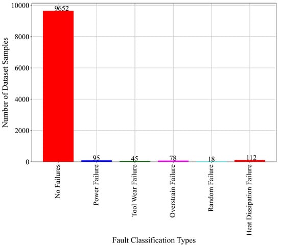
Figure 5.
The initial number of samples per class in “Fault Type” variable, which will be used in investigation of fault classification.
From Figure 5, it can be noticed that the class No Failure (Class_0) contains the largest number of samples in the dataset (9652). The other Failure Types classes contain an extremely low number of samples compared to the No Failure class. The Power Failure (Class_1) contains 95 dataset samples, the Tool Wear Failure (Class_2) contains 45 dataset samples, and the Overstrain Failure (Class_3) contains 78 dataset samples. The lowest number of dataset samples contains Random Failure (Class_4) (18), while the Heat Dissipation Failure (Class_5) contains the largest number of samples (115) when compared to other Failure Type classes. Figure 5 and the results showed that the dataset is highly imbalanced and the application of dataset balancing methods is mandatory since the training of any AI algorithm with an imbalanced dataset is not recommended as the trained algorithm might be biased toward the class with the higher number of samples.
Another problem that arises from the GPSC is that this algorithm cannot handle multiple classes in the target variable, so the one-versus-rest approach will be applied to each class in the target variable to transform the initial multi-class variable containing 5 classes to 5 binary classification target variables in the following way:
- No Failure (Class_0)—All the dataset samples that are some type of Failure Type will be labeled as 0 while the No Failure class will be labeled as 1. So, the number of samples for this new class is Failure-348 and No Failure-9652.
- Power Failure (Class_1)—In the new binary classification target variable of the same name, all the dataset samples that do not belong to that class will be named No Power Failure and labeled 0 (9905 samples) while Power Failure class samples will be labeled as 1 (95 samples).
- Tool Wear Failure (Class_2)—In the new binary classification target variable of the same name, all the dataset samples that do not belong to that class will be named No Tool Wear Failure and labeled 0 (9955) while the Tool Wear Failure class will be labeled as 1 (45 samples).
- Overstrain Failure (Class_3)—The new binary classification target variable of the same name will contain two classes, i.e., No Overstrain Failure labeled 0 (9922 samples) while the Overstrain Failure class will be labeled as 1 (78 samples).
- Random Failure (Class_4)—The new binary classification target variable of the same name will contain two classes, i.e., No Random Failure labeled 0 (9982 samples) while Random Failure class samples will be labeled as 1 (18 samples).
- Heat Dissipation Failure (Class_5)—The new binary classification target variable of the same name will contain two classes, i.e., No Heat Dissipation Failure labeled 0 (9888 samples) while Heat Dissipation Failure samples will be labeled 1 (112 samples).
With the application of the one-versus-rest approach from the target variable with 6 classes, the 6 binary classification target variables were created, i.e., 6 different datasets. However, these target variables are highly imbalanced, so the application of oversampling techniques is mandatory.
This dataset is definitely a challenge for dataset balancing techniques. The application of undersampling techniques was not considered in this manuscript since this type of technique would generate a very small dataset with insufficient data for training of the GPSC, and oversampling would definitely occur. The other problem with undersampling techniques is to achieve the balanced dataset variations since it requires extensive parameter tuning, which would not always guarantee the balanced dataset variation.
The question is if the application of oversampling techniques with small samples in the target class could achieve balanced dataset variations using whichever GPSC would not generate overfitted SEs. This is especially valid for datasets where Random Failure is the target since it only contains 18 samples in total.
2.3. Description of Dataset Preprocessing Techniques
In this subsection, the dataset preprocessing techniques will be described, i.e., scaling/normalization techniques as well as oversampling techniques.
The scaling/normalization techniques in combination with oversampling techniques were used to create a large dataset diversity which would later lead to a large number of trained ML models using whichever ensembles could be created that achieve a high and robust classification performance.
The oversampling techniques were chosen since the balance between classes in the target variable is easier to achieve than undersampling techniques even with the default parameters. It should be noted that the application of undersampling techniques on this dataset would lead to a dataset with an extremely small number of samples (e.g., the binary classification dataset for Class_4 would contain a total of 36 samples) that would be useless for training and might lead to overfitting.
2.3.1. Scaling/Normalization Techniques
In machine learning, data scaling is a crucial preprocessing step to normalize feature ranges and improve the performance of models. Scalers like MaxAbsScaler, MinMaxScaler, Normalizer, PowerTransformer, RobustScaler, and StandardScaler serve different purposes based on the nature of the data [17]. The MaxAbsScaler scales data by dividing each feature by its maximum absolute value, ensuring that all features fall within the range [−1, 1] without shifting the data’s mean. It is particularly useful for datasets with sparse features where preserving zero entries is important. The MinMaxScaler rescales features to a user-defined range, typically [0, 1], by transforming each feature based on its minimum and maximum values. This method is sensitive to outliers but ensures that all features lie within the specified range.
The Normalizer works differently; it scales each data point (row) individually to have a unit norm, effectively projecting the feature vector onto a unit hyper-sphere. This is ideal for algorithms sensitive to vector magnitudes, such as k-nearest neighbors or clustering. The PowerTransformer, on the other hand, applies a power-based transformation (e.g., Yeo–Johnson or Box–Cox) to stabilize variance and make the data more Gaussian-like, which can improve the performance of linear models on skewed data. The RobustScaler offers resilience against outliers by scaling data based on the interquartile range (IQR) rather than the mean and standard deviation, making it effective for datasets with extreme values. Lastly, the StandardScaler standardizes features by removing the mean and scaling them to unit variance, ensuring a distribution with a mean of 0 and a standard deviation of 1. This method is widely used in machine learning as it works well with algorithms that assume normally distributed data, such as logistic regression and Support Vector Machines. Each scaler has a specific role and is chosen based on the dataset’s characteristics and the requirements of the machine learning algorithm.
2.3.2. Oversampling Techniques
SMOTE is a foundational oversampling technique that generates synthetic data points for the minority class [18]. Instead of duplicating existing data, SMOTE creates new samples by interpolating between a minority class instance and its nearest neighbors. For each minority instance, synthetic examples are generated along the line connecting it to one or more of its k-nearest neighbors in feature space. This helps reduce overfitting caused by simple replication while ensuring better representation of the minority class.
ADASYN builds upon SMOTE by focusing on generating synthetic samples for the most challenging areas of the minority class [19]. It adaptively creates more synthetic examples near the decision boundary, where instances are harder to classify. This is achieved by weighting the minority samples based on their difficulty, such that instances with fewer nearby neighbors (in an imbalanced dataset) receive more attention. ADASYN enhances the learning process by addressing the bias introduced by class imbalance while maintaining better class distribution in the dataset.
BorderlineSMOTE is a variation of SMOTE that specifically targets the minority instances near the decision boundary between classes [20]. These instances, considered more likely to be misclassified, are oversampled to strengthen the classifier’s ability to distinguish between classes. BorderlineSMOTE creates synthetic samples only for those minority class instances that are identified as near or within the boundary region, thus improving the classifier’s performance where it matters most.
KMeansSMOTE combines the principles of clustering and oversampling to generate synthetic minority class samples [21]. It applies k-means clustering to divide the minority class into clusters and then applies SMOTE within each cluster. This ensures that synthetic samples are generated in a way that preserves the underlying distribution of the minority class, making it particularly effective when dealing with datasets where the minority class exhibits complex substructures.
SVMSMOTE uses a Support Vector Machine (SVM) to identify the minority class instances that are closest to the decision boundary (support vectors) [22]. These support vectors are then used to generate synthetic samples. By focusing on instances near the boundary, SVM-SMOTE ensures that the new samples are strategically placed to improve the classifier’s performance, especially in cases of highly overlapping classes. This targeted oversampling approach enhances the ability of the model to differentiate between the classes.
2.4. The Results of Dataset Preprocessing Techniques
In the case of fault detection, the number of samples that belong to Not Failure (label 0) and Failure (label 1) in balanced dataset variations after application of scaling/normalization and oversampling techniques is shown in Figure 6.
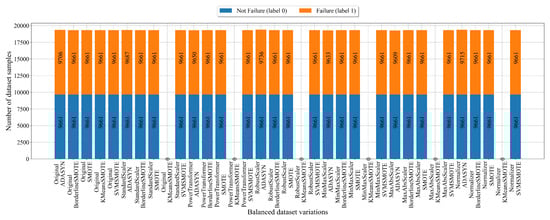
Figure 6.
The balanced dataset variation of dataset with fault detection as the target variable obtained using scaling/normalization and oversampling techniques.
As seen in Figure 6, the KMeansSMOTE method could not produce an equal number of samples, i.e., the same number of No Failure and Failure classes so the value is 0. The only occurrence where KMeansSMOTE did achieve balance is in the case of the dataset for fault detection with original values. The application of the ADASYN technique achieved balance between class samples; however, the difference between samples is almost negligible when compared to the initial imbalance (0–9661, 1–339). Using BorderlineSMOTE, SMOTE, and SVMSMOTE, perfectly balanced dataset variations were created.
In case of fault classification, the “Failure Type” class initially contained 6 different classes. Since the GPSC could not handle the multi-class target variable, the multi-class variable was broken down into 6 binary target variables, one target variable for each class using a one-versus-rest approach as explained earlier. The results of the application of the scaling/normalization techniques as well as the oversampling techniques for Class_0 (No Failure) are shown in Figure 7.
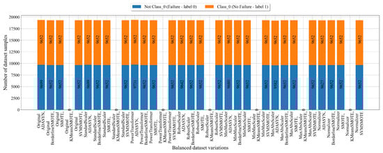
Figure 7.
The balanced dataset variation of dataset with Class_0 (No Failure) as the target variable obtained using scaling/normalization and oversampling techniques.
The balanced dataset variations with Class_0 as the target variable shown in Figure 7 are perfect when using BorderlineSMOTE, SMOTE, and SVMSMOTE. The KMeansSMOTE was unable to achieve the balance between classes, so the values are 0. The ADASYN technique balanced the scaled/normalized dataset variations; however, there is still a small difference between class samples.
The number of samples per class in balanced dataset variations obtained for Class_1 (Power Failure) is shown in Figure 8.
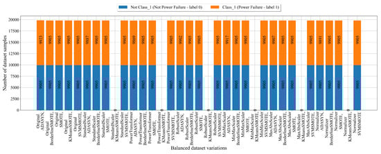
Figure 8.
The balanced dataset variation of dataset with Class_1 (Power Failure) as the target variable obtained using scaling/normalization and oversampling techniques.
The KMeansSMOTE failed to balance all preprocessed dataset variations except the dataset with original values, as shown in Figure 8. The ADASYN technique achieved the balance with a small difference between class samples. For example, the Original_ADASYN contains 9905 samples from Not Class_1 and 9923 samples from Class_1. The difference is small; however, this is still an amazing result since the imbalanced dataset contained only 95 samples.
The number of samples in the balanced dataset variations for Class_2 after the application of scaling/normalization and oversampling techniques is shown in Figure 9.
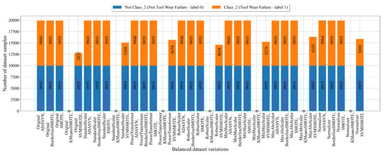
Figure 9.
The balanced dataset variation of dataset with Class_2 (Tool Wear Failure) as the target variable obtained using scaling/normalization and oversampling techniques.
The SVMSMOTE technique showed odd behavior in the case of Class_2, as shown in Figure 9, since it was unsuccessful in balancing the dataset. The KMeansSMOTE did not achieve the balanced dataset variations, so the value is 0. ADASYN showed similar behavior as before. The only two techniques that perfectly balanced the Not Class_2 with Class_2 samples are BorderlineSMOTE and SMOTE, which achieved perfect balance.
The number of samples in balanced dataset variations for Class_3 after the application of scaling/normalization and oversampling techniques is shown in Figure 10.
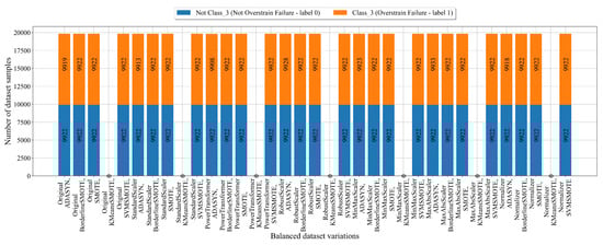
Figure 10.
The balanced dataset variation of dataset with Class_3 (Overstrain Failure) as the target variable obtained using scaling/normalization and oversampling techniques.
The balanced dataset variations obtained with the scaling/normalization and oversampling techniques shown in Figure 10 have the same trend as in the case of Class_0 and 1. This means the KMeansSMOTE failed, ADASYN generated a balanced dataset but with small differences between class samples, and BorderlineSMOTE, SMOTE, and SVMSMOTE generated perfect balanced dataset variations.
The number of samples in balanced dataset variations for Class_4 after applications of scaling/normalization and oversampling techniques is shown in Figure 11.
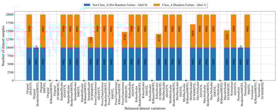
Figure 11.
The balanced dataset variation of dataset with Class_4 (Random Failure) as the target variable obtained using scaling/normalization and oversampling techniques.
The balanced dataset variations obtained for Class_4 (Figure 11) showed that only SMOTE was able to achieve the balance between class samples regardless of the scaling/normalization previously applied. BorderlineSMOTE and SVMSMOTE could not achieve the balanced dataset variations, so they should be omitted from further analysis.
The number of samples in balanced dataset variations for Class_5 after the application of scaling/normalization and oversampling techniques is shown in Figure 12.
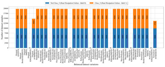
Figure 12.
The balanced dataset variation of dataset with Class_5 (Heat Dissipation Failure) as the target variable obtained using scaling/normalization and oversampling techniques.
In the case of balanced dataset variations for Class_5 (Figure 12), the ADASYN, BorderlineSMOTE, and SMOTE techniques achieved balanced dataset variations. The KMeansSMOTE and SVMSMOTE technique failed to achieve balanced dataset variations.
It should be noted that the GPSC will be trained on all these balanced dataset variations using 5FCV, while the GPSC hyperparameters will be searched for using the RHVS method.
2.5. Genetic Programming Symbolic Classifier with Random Hyperparameter Values Search Method
The genetic programming symbolic classifier is an evolutionary algorithm that begins the execution by generating the population of naive symbolic expressions (SEs) [23]. These SEs are unfit for the particular task; however, with the application of the genetic operations such as crossover and mutation, they are eventually fit for the particular task. The benefit of the GPSC is the ability to, after training, obtain the best SEs of the training process that can perform the particular classification task [23]. The GPSC has a large number of hyperparameters [24], and these are as follows:
- PS—The size of the initial population [24].
- GenMax—The maximum number of generations. This hyperparameter is also one of the GPSC termination criteria, and if reached, the GPSC execution is terminated [24].
- DepthInit—The initial depth of the population members. The population members in the GPSC are represented as tree structures, and the size of the population members can be measured with the depth of the population member starting from a root node, which is 0. It should be noted that DepthInit is defined as the range from the minimum to the maximum value. This reason why this hyperparameter is in range is due to the fact that the method used to create the initial population requires the definition of this hyperparameter in this way. The method is ramped half-and-half, which combines two of the oldest methods, the full and grow method, and the depth of the population members is in range, hence the term ramped [24].
- TS—The tournament size hyperparameter value that defines the size of the tournament selection. The size must always be less than the population size [24].
- Stopping criteria—Another GPSC termination criterion, and this hyperparameter is the predefined minimum value of the fitness function. If this value is reached by one of the population members during the GPSC execution, the GPSC execution is terminated. It should be noted that the fitness function in the GPSC is measured with the binary cross-entropy loss function. To measure the binary cross-entropy loss value for one population member in the GPSC, first, input values from the training set are provided to compute the output. Then, this output is used as input in the Sigmoid function:where x is the output of the population member [25]. When Sigmoid is applied to all the outputs generated by the population member, this output, along with the size of the real (target) values from the dataset, is used to compute the binary cross-entropy loss. The binary cross-entropy loss function [26] is defined aswhere
- -
- is the true label (0 or 1).
- -
- is the predicted probability (the output of the Sigmoid function).
- -
- N is the total number of samples.
- CrossProb—The crossover probability value and one of the genetic operations, which requires two winners of the tournament selection. The random selection of subtrees is performed on both population members, and the subtree of the second tournament selection winner replaces the subtree of the first tournament selection winner [24].
- SubtreeMute—The subtree mutation probability value of the genetic operation that requires only one tournament selection winner. The random subtree is selected on the winner and replaced with a randomly generated subtree from the primitive set [24].
- HoistMute—The probability of the hoist mutation operation, which requires only one population member. The hoist mutation randomly selects a subtreee and randomly selects a node on that subtree. Then, the node replaces the entire subtree [24].
- PointMute—The probability of the point mutation operation; also requires one tournament selection winner, and on that winner, random nodes are selected. The mathematical functions are replaced with other mathematical functions; however, the number of arguments must be the same. The constant values are replaced with randomly selected constant values from the constant range. The input variables are replaced with other randomly selected variables [24].
- MaxSamples—The maximum percentage of samples that will be used for training of the GPSC while the remaining part will be used for testing. Generally, it is good practice to leave at least 1 to 0.1% of the dataset to see how population members perform on the unseen data. In practice, the fitness function of population members on the training data and the test data (out-of-bag fitness) should be similar. If these values largely deviate, this can cause overfitted models [24].
- ParsCoef—The coefficient of the parsimony pressure method. This method penalizes large SEs by increasing the fitness value and thus makes them least favorable for selection. It is one of the most sensitive parameters to tune [24].
- ConstRange—The range of constant values [24].
It should be noted that the GPSC also requires the definition of mathematical functions, which will be used to develop the initial population and for all mutation operations inside the GPSC algorithm. In this investigation, the following mathematical functions are used: addition, multiplication, subtraction, division, natural logarithm, logarithms with bases 2 and 10, cube root, square root, sine, cosine, tangent, and absolute value. However, some mathematical functions had to be slightly modified to avoid generating a number of ∞ values, which could potentially lead to an error that will terminate the GPSC execution. The description of these modified mathematical functions is given in Appendix A. To find the optimal combination of the GPSC hyperparameters, the random hyperparameter values search (RHVS) method was developed, tweaked, and used. This method consists of the following steps:
- Define the lower and upper boundary for each hyperparameter.
- Test the performance of each hyperparameter value, and if the GPSC did not successfully execute, modify the boundaries.
After initial testing and adjustment of the GPSC hyperparameter boundary values, the boundaries for each hyperparameter that will be used in the RHVS method are listed in Table 3.
Table 3.
The boundary values of each GPSC hyperparameter that will be used in RHVS method.
From Table 3, it can be noticed that subtree mutation (SubtreeMute) probability will be dominating the genetic operation since the probability values are in 0.95 to 1.0 range. This range was set due to the fact that the initial investigation showed that subtree mutation is a more aggressive mutation operation than other mutation operations, and compared to crossover, is memory efficient since it requires only one TS winner to perform a mutation operation. The parsimony coefficient (ParsCoeff) value was set to the and range, i.e., a very narrow range. Smaller values contributed to generating very large SEs while higher values choked the evolution process i.e., the growth of SEs. The stopping criteria value was set to extremely small values since the initial investigation showed that higher values prematurely terminated GPSC execution.
2.6. Evaluation Metrics
To evaluate the SEs and the TBVE, in this paper, the accuracy (ACC), area under the receiver operating characteristics curve (AUC), precision score, recall score, F1-score, and confusion matrix. However, before explaining the aforementioned evaluation metric methods, the basic elements that these metrics use in their calculation, such as true positive (TP), true negative (TN), false positive (FP), and false negative (FN), will be explained first.
- TP—The SE correctly predicts the positive class when the sample from the dataset is also positive. For example, the SE detects machine failure (positive) when the actual value is positive.
- TN—The SE correctly predicts the negative class when the actual class is negative. The SE correctly identifies the machine without failures (negative) when the machine indeed operates normally without failures.
- FP—The SE incorrectly predicts a positive class when the actual class is negative. The SE detects machine failure (positive) while the actual value is a machine with normal operation (negative), resulting in a false alarm.
- FN—The SE incorrectly predicts a negative class when the actual class is positive. In the case of machine failure, the SE predicts that there is No Failure when the actual value is positive, i.e., the failure in the machine occurred.
The ACC is the evaluation metric that measures the proportion of correctly predicted samples (TP and TN) out of the total samples in the dataset [27]. The ACC is calculated using the following expression:
where , , , and denote true positive, true negative, false positive, and false negative, respectively. These four components were defined earlier. The high ACC indicates that the model is making correct predictions most of the time. However, the ACC alone can be misleading, especially in the imbalanced datasets.
The AUC is the evaluation metric value used to evaluate the quality of a binary classification model by measuring the ability to distinguish between two classes. The AUC is the total area under the ROC curve, representing the model’s ability to separate the positive and negative classes across all thresholds [28]. An AUC of 1.0 indicates an SE with a perfect classification performance, with no overlap between classes, i.e., the SE correctly classifies all positives and negatives. An AUC of 0.5 indicates a model with no discrimination ability, equivalent to random guessing. An AUC in the 0.5 to 1.0 range represents the SE that has some discriminatory power but is not perfect. The closer the AUC is to 1.0, the better the SE performs in distinguishing between classes.
The precision score is the evaluation metric value that measures the accuracy of positive predictions, focusing on how many of the samples predicted as positive are actually positive [29]. The precision score is calculated using the following expression:
The high precision means that the models make few false positive errors.
The recall score is the evaluation metric method that measures the SEs’ ability to identify all actual positives in the dataset [29]. The recall score is calculated using the following expression:
The high recall score indicates that the model captures almost all positive samples with few false negatives.
The F1-score is the harmonic mean of the precision and recall, providing a single metric that balances both [30]. The F1-score is measured using the following expression:
The F1-score ranges from 0 to 1, where 1 represents perfect precision and recall. The high F1-score is achieved only if both precision and recall are high, making it useful when the balance between them is needed, especially when dealing with imbalanced datasets.
The confusion matrix is a table that visualizes the performance of a classification model by comparing the predicted values against the actual values [31]. In the case of a binary classification problem, the confusion matrix has four components, as shown in Table 4.
Table 4.
The demonstration of error types.
2.7. Training Testing Procedure
The graphical illustration of the train–test procedure is shown in Figure 13.
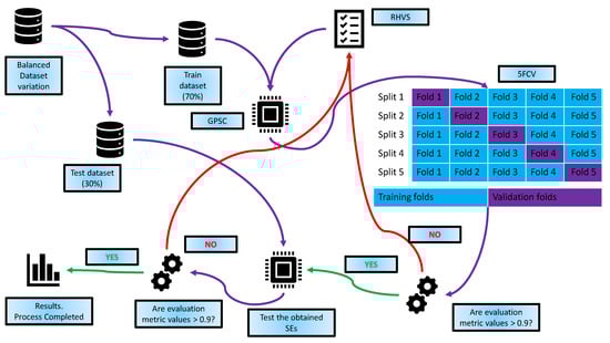
Figure 13.
The graphical illustration of train–test procedure.
The training–testing procedure graphically illustrated in Figure 13 consists of the following steps:
- The balanced dataset variation is divided into the train–test dataset in a ratio of 70:30. Besides the train–test dataset, the random hyperparameter values are selected using the RHVS method.
- The GPSC is trained using 5FCV where, for each split, an SE is generated, so for 5 splits, a total of 5 SEs are obtained. Besides the SEs at this step, the evaluation metric values are obtained on the train and validation folds inside the 5FCV.
- After the 5FCV process is completed and the SEs are obtained, the mean and standard deviation values are obtained. If the values are higher than 0.9, the process proceeds to the test phase; if they are lower than 0.9, the process starts from the beginning with the random selection of GPSC hyperparameter values using the RHVS method.
- If eventually the process reaches the test phase, a test dataset (30%) is provided to obtain SEs to compute the output. After the output is obtained, they are used to calculate the evaluation metric values. If the evaluation metric values are all higher than 0.9, the process is completed, and the best set of SEs is obtained for balanced dataset variation on which the GPSC was trained. If the evaluation metric values are lower than 0.9 then the process starts from the beginning with random selection of GPSC hyperparameter values using the RHVS method.
2.8. Threshold-Based Voting Ensemble
The Threshold-Based Voting Ensemble (TBVE) is a method designed to enhance the performance and reliability of machine learning models by combining the outputs of multiple classifiers. In the context of this study, the TBVE integrates symbolic expressions (SEs) obtained from genetic programming symbolic classifiers (GPSCs) trained on balanced dataset variations. Each SE acts as an independent classifier, providing a prediction for a given input. The ensemble’s decision-making process is governed by a threshold parameter that determines the minimum number of SEs required to agree on a class label for it to be assigned as the final prediction.
The TBVE operates by aggregating predictions from the SEs and counting the votes for each class. If the number of votes for a specific class exceeds the threshold value, that class is selected as the final output. By adjusting the threshold, the TBVE can control the trade-off between sensitivity and specificity, allowing for the fine-tuning of the classification performance. Lower thresholds increase sensitivity, reducing false negatives, while higher thresholds enhance specificity, minimizing false positives. This flexibility makes the TBVE a robust and explainable approach, capable of leveraging diverse perspectives from individual SEs while maintaining high classification accuracy and reliability for failure detection and classification in machine predictive maintenance applications.
2.9. Alternative Approach with RFC
In scenarios where the Threshold-Based Voting Ensemble (TBVE) constructed from a genetic programming symbolic classifier (GPSC) symbolic expressions (SEs) does not yield satisfactory results, an alternative strategy is pursued. In this approach, the outputs of the SEs are utilized as inputs to train the Random Forest Classifier (RFC).
To ensure the best performance, the outputs obtained from SEs undergo preprocessing, including scaling or normalization using one of the following techniques: MaxAbsScaler, MinMaxScaler, Normalizer, PowerTransformer, RobustScaler, or StandardScaler. Subsequently, due to the inherent class imbalance in the dataset, oversampling techniques are employed. The methods considered include Adaptive Synthetic Sampling (ADASYN), Borderline Synthetic Minority Oversampling Technique (BorderlineSMOTE), KMeansSMOTE, SMOTE, and Support Vector Machine SMOTE (SVMSMOTE). This combination of scaling/normalization and oversampling results in multiple balanced dataset variations.
Each of these variations is used to train the RFC, with hyperparameter tuning carried out via the RandomizedSearchCV method to optimize model performance. The best model obtained from each variation is preserved. Subsequently, for each class, the models trained on the various balanced dataset variations are utilized to construct and evaluate a new TBVE on the original, imbalanced dataset.
The hyperparameters of the RFC are explored using the following parameter grid (Table 5).
Table 5.
Hyperparameters of Random Forest Classifier for RandomizedSearchCV.
The hyperparameters are defined as follows:
- n_estimators: The number of trees in the forest. Increasing this value can improve accuracy but may increase computation time.
- max_depth: Controls the maximum depth of each decision tree. Deeper trees can model more complex relationships but may lead to overfitting.
- min_samples_split: Specifies the minimum number of samples required to split an internal node. Higher values help prevent overfitting.
- min_samples_leaf: Determines the minimum number of samples required to be at a leaf node. Larger values can smooth the model, reducing variance.
- bootstrap: Determines whether bootstrap sampling is used. When set to True, it enables bagging, which helps reduce overfitting.
By combining the RFC models obtained from each balanced dataset variation and integrating them into a new TBVE, we aim to enhance the classification performance on the initial imbalanced dataset.
2.10. Computational Resources
All experiments in this study were conducted on a desktop workstation equipped with an AMD Ryzen 7 3800X 8-core, 16-thread processor, and 32 GB of DDR4 RAM. No GPU acceleration was used, as the methodology was designed to operate efficiently on standard CPU-based systems, demonstrating its practicality for deployment in resource-constrained environments.
The implementation was carried out using the Python programming language (version 3.12). The following open-source libraries were used:
- scikit-learn for classification algorithms (Random Forest), model evaluation (cross-validation and performance metrics), hyperparameter optimization (RandomizedSearchCV), and data preprocessing (scaling and normalization).
- gplearn for symbolic regression and the development of the genetic programming symbolic classifier (GPSC), which was extended to suit the classification task.
- imbalanced-learn for oversampling techniques to address class imbalance.
- NumPy and Pandas for efficient numerical computation and data manipulation.
The total computation time for training the GPSC across all dataset variations (including 5-fold cross-validation and hyperparameter search) spanned approximately 145 h (6.4 days). Despite this, each model was trained offline and independently, allowing the process to be parallelized and automated for large-scale deployment.
All experiments were reproducible and executed in a controlled environment without external cloud computing resources, highlighting the approach’s feasibility for practical industrial use.
3. Results
The results section is divided into three main subsections, and these are as follows:
- The analysis of the classification performance of the SEs achieved on balanced dataset variations and optimal combinations of GPSC hyperparameter values using the RHVS that was used to obtain SEs.
- The analysis of the SEs with a high classification performance.
- The development of a meta-dataset using the SE output.
- The classification performance of the RFC on balanced dataset variations.
- The development of a TBVE based on the RFC trained models.
3.1. The Analysis of the SEs Obtained on Balanced Dataset Variations for Fault Detection
The classification performance of the best SEs obtained on each balanced dataset variations using the GPSC is shown in Figure 14.
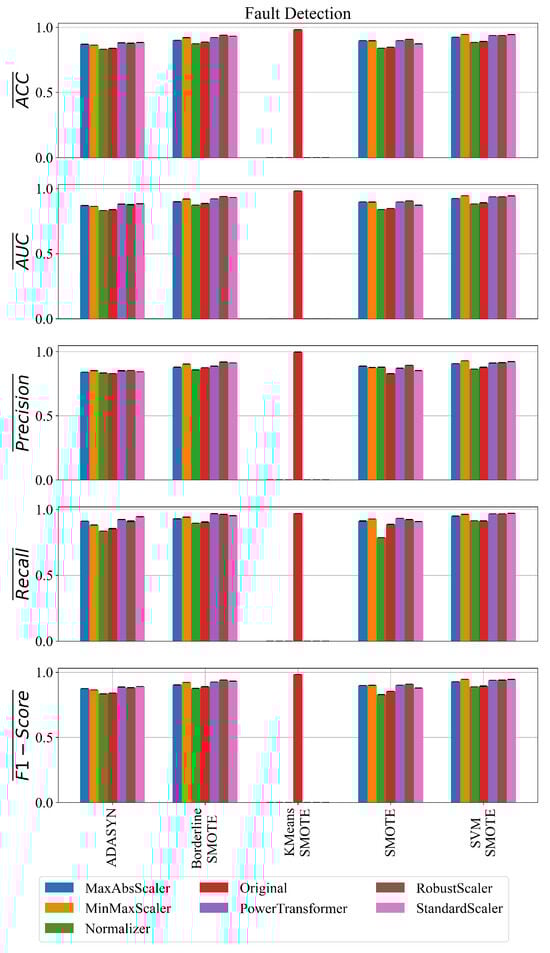
Figure 14.
The classification performance of the best SEs obtained on each balanced dataset variation with GPSC for fault detection.
As seen from Figure 14, the SEs obtained on the datasets balanced with SVMSMOTE consistently produced top results regardless of scaler (especially with MinMaxScaler and PowerTransformer), showing high precision, recall, and F1-score. The example is the SEs obtained on the MinMaxScaler_SVMSMOTE dataset where the SEs achieved ACC = 0.9448, F1-score = 0.9458, and AUC = 0.9448. The SEs obtained on the BorderlineSMOTE also performed very well, especially in the case of the Standard and Robust Scaler (F1-score = 0.9406) and PowerTransformer (F1-score = 0.9253). ADASYN and Normalizer combinations generally underperform with lower accuracy and recall, e.g., Normalizer_ADASYN with ACC = 0.831 and F1-score = 0.834.
The SEs obtained on Original_KMeansSMOTE achieved an extremely high classification performance. It is an outlier with extremely high results, which indicates that overfitting occurred and these equations were neglected from further analysis.
Regarding the stability of the obtained results, the SEs obtained on the SVMSMOTE datasets have very low variance, showing consistent behavior. The PowerTransformer_SVMSMOTE has an F1-score of 0.00017, which can be classified as very stable. The Normalizer_BorderlineSMOTE also shows the low stds across all metrics.
Due to a large number of SEs obtained on all balanced dataset variations, there is also a large number of optimal combinations of GPSC hyperparameter values that were found using the RHVS method. So, in Table 6, the results of the statistical analysis of the optimal combination of GPSC hyperparameter values obtained for each balanced dataset variation through the RHVS method are shown.
Table 6.
The statistical analysis of optimal combination of GPSC hyperparameter values found using RHVS method on each balanced dataset variation.
In Table 6, the population size (PopSize) and maximum generations (MaxGen) show high variability (std = 333.280 and 34.305, respectively), suggesting flexibility in achieving optimal results with different evolutionary durations and population scales. However, some extreme values (Min = 0 for both) may indicate occasional early convergence or redundant optimization. Similarly, tournament size (TourSize) also exhibits wide dispersion (mean = 298.314 and std = 155.409), reflecting its influential but dataset-sensitive nature.
The initial tree depth parameters (InitD_Lower and InitD_Upper) average around 4.1 and 12.5, respectively, indicating that deeper trees are often beneficial for capturing complex patterns, though their use is context-dependent, as evidenced by the relatively large standard deviations.
Among mutation rates, subtree mutation (SubMute) dominates (mean = 0.798), while Crossover, hoist mutation, and point mutation rates are minimal (0.01), emphasizing the central role of subtree mutation in exploration, with other genetic operations contributing minimally.
The stopping criterion (StopCrit) and parsimony coefficient (ParsCoeff) remain negligible, reinforcing the preference for full evolution cycles without early termination or parsimony pressure. The max samples (MaxSamp) mean of 0.824 indicates a tendency toward large subsample sizes, favoring generalization.
Lastly, the constant range bounds (ConstRange_Lower = –475.396, ConstRange_Upper = 375.563) show high variability, suggesting that allowing wide numeric ranges helps capture dataset-specific relationships but may require careful constraint tuning to avoid overfitting.
In summary, the analysis highlights the adaptability of the GPSC, where larger population sizes, deeper trees, dominant subtree mutation, and wide constant ranges contribute to robust performance across balanced variations, with considerable tuning flexibility depending on the dataset characteristics.
3.2. The Analysis of the SEs Obtained on Balanced Dataset Variations for Fault Classification
The classification performance of the SEs obtained on balanced dataset variations using GPSC + RHVS + 5FCV for each class is shown in Figure 15 and Figure 16.
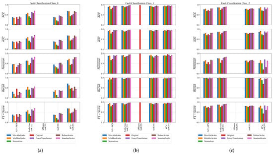
Figure 15.
The classification performance of SEs obtained on balanced dataset variations for Classes 0, 1, and 2. (a) The classification performance of SEs obtained on balanced dataset variations of Class_0; (b) the classification performance of SEs obtained on balanced dataset variations of Class_1; (c) the classification performance of SEs obtained on balanced dataset variations of Class_2.
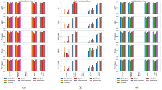
Figure 16.
The classification performance of SEs obtained on balanced dataset variations for Classes 3, 4, and 5. (a) The classification performance of SEs obtained on balanced dataset variations of Class_3; (b) the classification performance of SEs obtained on balanced dataset variations of Class_4; (c) the classification performance of SEs obtained on balanced dataset variations of Class_5.
Figure 15a presents the classification performance across various scaling and oversampling combinations for Class_0 using metrics such as accuracy (ACC), AUC, precision, recall, and F1-score. The best results were achieved using SVMSMOTE in combination with StandardScaler and RobustScaler. Both configurations yielded high accuracy (0.9346), AUC (0.9348), precision (0.9589), recall (0.9092), and F1-score (0.9334), demonstrating their effectiveness in handling class imbalance. PowerTransformer with BorderlineSMOTE also performed well (ACC = 0.9272, F1 = 0.9248), particularly excelling in precision (0.9555). Other strong performers included MinMaxScaler and StandardScaler with BorderlineSMOTE, showing balanced precision and recall. All KMeansSMOTE combinations failed to produce valid results, suggesting poor compatibility in this context. ADASYN configurations showed a moderate performance, with the best results from RobustScaler and StandardScaler (ACC 0.8806, F1 0.8778), though with lower recall. Similarly, SMOTE showed an average performance across most scalers. In summary, SVMSMOTE combined with appropriate scaling consistently outperformed other oversampling techniques, particularly when paired with StandardScaler, RobustScaler, or PowerTransformer.
The classification results obtained using SEs for Class_1 across various balanced dataset variations (Figure 15b) demonstrate a consistently strong performance, with several configurations achieving near-perfect scores. Among all combinations, the best results were observed with the Original_KMeansSMOTE dataset, which yielded almost perfect classification metrics, including an accuracy and F1-score of approximately 0.995. Similarly, PowerTransformer_SVMSMOTE also stood out, achieving an accuracy of 0.9918, precision of 0.9844, recall of 0.9995, and an F1-score of 0.9919, indicating excellent balance between sensitivity and specificity.
Other high-performing setups included RobustScaler_BorderlineSMOTE and StandardScaler_BorderlineSMOTE, both of which delivered F1-scores above 0.992, showcasing their robustness in handling class imbalance when paired with SEs. Across the board, SMOTE and SVMSMOTE, when used with scalers like MinMaxScaler, StandardScaler, and RobustScaler, also produced highly reliable results with F1-scores consistently ranging between 0.985 and 0.990. ADASYN-based variations generally provided slightly lower precision but compensated with very high recall, especially when paired with PowerTransformer and RobustScaler.
In contrast, all variations involving KMeansSMOTE, except when combined with the original unscaled data, failed to produce any meaningful results—returning zero values for all performance metrics—suggesting a critical incompatibility or preprocessing failure with this specific oversampling technique. Overall, the experiments confirm that SEs are highly effective for classifying Class_1 in balanced datasets, especially when combined with SVMSMOTE, BorderlineSMOTE, and scaling techniques like PowerTransformer or RobustScaler.
The classification performance of the SEs obtained for Class_2 (Figure 15c), obtained on balanced dataset variations, indicates strong and consistent results, particularly when using SMOTE variants combined with effective scaling techniques. The best overall performance was observed with StandardScaler_BorderlineSMOTE, achieving a high mean accuracy of 0.979 and F1-score of 0.9793, demonstrating an excellent balance between precision and recall. Similarly, RobustScaler_BorderlineSMOTE and PowerTransformer_BorderlineSMOTE also delivered top-tier results, with F1-scores exceeding 0.975, indicating that BorderlineSMOTE is a reliable oversampling method when paired with proper normalization.
A good performance was also observed with MinMaxScaler_SVMSMOTE and PowerTransformer_SVMSMOTE, achieving F1-scores around 0.96, reflecting high classification reliability. Other combinations, such as RobustScaler_SMOTE, StandardScaler_ADASYN, and MinMaxScaler_SMOTE, consistently yielded F1-scores in the 0.959–0.964 range, confirming their robustness.
In contrast, all KMeansSMOTE-based variations failed to produce any viable results, with all metrics equal to zero, indicating issues with model training or oversampling compatibility. Overall, SEs proved highly effective for Class 2 classification, especially when combined with BorderlineSMOTE or SVMSMOTE and scaling methods such as StandardScaler, RobustScaler, or PowerTransformer.
The classification performance of the obtained SEs on balanced dataset variations using the GPSC for Classes 3, 4, and 5 is shown in Figure 16.
The best SEs obtained for Class 3 demonstrate an excellent classification performance across different preprocessing and oversampling techniques, as shown in Figure 16a. The best results, particularly with StandardScaler and MinMaxScaler combined with BorderlineSMOTE or ADASYN, achieve mean accuracies and AUC values above 0.995. Precision scores consistently exceed 0.98, while recall values are exceptionally high, often nearing 1.0, indicating strong true positive detection. F1-scores closely follow accuracy, reflecting a balanced performance. Low standard deviations across all metrics show that the models are stable and reliable. Some oversampling methods, like KMeansSMOTE, failed to produce results, but overall, the top-performing SEs offer robust and consistent classification for Class 3.
The best SEs obtained for Class 4 on balanced dataset variations (Figure 16b) show a varied performance depending on the preprocessing and oversampling methods used. The best results come from combinations like StandardScaler, MinMaxScaler, and RobustScaler with BorderlineSMOTE or SVMSMOTE, achieving high mean accuracies around 0.98 to 0.99, an excellent precision above 0.95, and near-perfect recall values close to 1.0. These lead to strong F1-scores around 0.97 to 0.99, indicating well-balanced and reliable classification. Some oversampling methods like KMeansSMOTE and certain Normalizer variants failed to produce meaningful results, reflected by zeros across metrics. Overall, the SEs perform robustly with most advanced scalers and synthetic oversampling techniques, demonstrating stable and effective classification for Class 4.
The best SEs obtained for Class 5 on balanced dataset variations demonstrate a consistently high performance across various scaling and oversampling techniques (Figure 16c). Notably, the PowerTransformer combined with SMOTE achieved the highest metrics, with mean accuracy, AUC, precision, recall, and F1-score all exceeding 0.998, indicating near-perfect classification. Other strong performers include PowerTransformer with BorderlineSMOTE and RobustScaler with ADASYN, both yielding mean accuracies above 0.994 and similarly high precision and recall values. Across all top models, recall values approached or reached 1.0, highlighting excellent sensitivity in detecting Class 5 instances. StandardScaler and MaxAbsScaler variants also delivered robust results with mean accuracies above 0.99. These results confirm that the combination of effective scaling with advanced oversampling methods produces highly reliable SE-based classifiers for Class 5 in the balanced dataset scenario.
Due to a large number of classes and a large number of balanced dataset variations, the number of optimal combinations of the GPSC hyperparameter values is impossible to show. So, in Table 7, the statistics of optimal combinations of GPSC hyperparameter values for each class are listed.
Table 7.
Results of statistical analysis for optimal combinations of GPSC hyperparameter values for each class.
For Class 0 (Table 7), the optimal GPSC hyperparameters had an average population size of about 636 and around 63 generations, both with significant variability. The tournament size averaged approximately 281. Initialization depths ranged from about 4.1 (lower) to 12 (upper). The crossover rate was low (0.013), while subtree mutation was high (0.77). Hoist and point mutations were low but slightly higher than in some other classes (0.011 and 0.01). The stopping criterion was very small (0.0004), and maximum sample usage was high (0.80). Constant value ranges were broad, from roughly −434 to 358, and the parsimony coefficient was low (0.00037), reflecting a balanced but diverse search for optimal symbolic expressions.
For Class 1 (Table 7), the optimal GPSC hyperparameters showed an average population size of about 646 and roughly 65 generations, both with considerable variance. The tournament size averaged around 315. Initialization depths ranged from 3.8 (lower) to 12.3 (upper). The crossover rate was low (0.011), while subtree mutation was high (0.80). Hoist and point mutation rates remained low (0.009 and 0.01). The stopping criterion was small (0.00036), and maximum sample usage was relatively high (0.82). Constant ranges were wide, spanning roughly -421 to 414, and the parsimony coefficient was low (0.00041), indicating a focused yet diverse evolutionary strategy for optimal classification performance. For Class 2 (Table 7), the optimal GPSC hyperparameters had an average population size of about 658 and around 62 generations, both with high variability. Tournament size averaged 305, with initialization depths between 3.8 (lower) and 11.5 (upper). The crossover rate was low (0.008), subtree mutation high (0.77), while hoist and point mutations remained low (0.009 and 0.01). The stopping criterion was small (0.00049), and maximum sample usage was relatively high (0.80). Constant ranges were broad, from approximately −443 to 436, with a low parsimony coefficient (0.00036), reflecting a diverse but targeted evolutionary setup for best classification results.
For Class 3 (Table 7), the optimal GPSC hyperparameters showed an average population size of about 640 and around 60 generations, both with considerable variability. The tournament size averaged 297, with initialization depths roughly 4 (lower) to 12 (upper). Crossover rates were low (0.013), subtree mutation was high (0.77), while hoist and point mutations remained low (0.007 and 0.011). The stopping criterion was very small (0.00039), and maximum sample usage was relatively high (0.80). Constant ranges spanned widely from about -485 to 419, with a low parsimony coefficient (0.00036), indicating diverse yet focused evolutionary settings for optimal classification performance.
For Class 4 (Table 7), the optimal GPSC hyperparameters had an average population size of about 582 and around 58 generations, both with high variability. The tournament size averaged 276, with initialization depths ranging from 4 (lower) to about 11.5 (upper). Crossover rates remained low (0.012), subtree mutation was high (0.71), while hoist and point mutations were minimal (0.009 and 0.008). The stopping criterion was very small (0.00033), and maximum sample usage was moderately high (0.74). Constant ranges varied widely between roughly −392 and 385, with a low parsimony coefficient (0.00036), reflecting diverse yet targeted evolutionary settings for best performance.
The optimal GPSC hyperparameters for Class 5 on balanced datasets show high variability in population size (mean 613) and generations (mean 56) (Table 7). The tournament size averaged around 281, while initialization depths ranged broadly (lower 3.9 and upper 11.8). The crossover rates were very low (0.009), but subtree mutation was high (0.74), with hoist and point mutations used minimally (0.01). The stopping criterion was very small (0.00036), and maximum sample usage was generally high (0.77). Constant ranges varied widely, and the parsimony coefficient was consistently low (0.00035), indicating diverse yet focused evolutionary settings for best classification performance.
3.3. The Analysis of the Best SEs
In this section, only an example of SEs will be shown that were obtained using the GPSC on balanced dataset variation. The selected set of SEs with the highest classification performance will be evaluated on the imbalanced dataset to see how well it performs. The selected SEs are those obtained on the PowerTransformer+SMOTE dataset for Class_5. To compute the output for these equations, the dataset must be subjected to the PowerTransformer before using it. If the original values are used, the output might lead to a low classification performance. The equations are
As seen from Equations (7)–(11), the equations are pretty simple. To compute the output:
After the output is obtained from each equation to determine the class, this output must be used as input in the Sigmoid function Equation (1).
To evaluate the performance of the previously shown SEs, the SEs were evaluated on the imbalanced dataset for Class_5; however, the input variables had to be preprocessed with PowerTransformer. The results are shown in the form of CMs in Figure 17.
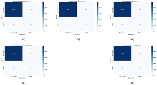
Figure 17.
The CMs obtained on imbalanced dataset for Class_5 using Equations (7)–(11). (a) Confusion matrix for Equation (7) evaluated on imbalanced dataset for detection of Class_5; (b) confusion matrix for Equation (8) evaluated on imbalanced dataset for detection of Class_5; (c) confusion matrix for Equation (9) evaluated on imbalanced dataset for detection of Class_5; (d) confusion matrix for Equation (10) evaluated on imbalanced dataset for detection of Class_5; (e) confusion matrix for Equation (11) evaluated on imbalanced dataset for detection of Class_5.
From Figure 17a, it can be noticed that Equation (7) successfully predicted all 112 samples that belong to Class_5 while 9814 out of 9888 samples were successfully predicted as Not Class_5 samples. The classification performance of Equation (8) presented in Figure 17b shows that the SE again successfully predicted 112 samples that do belong to Class_5 while 9834 out of 9888 samples were successfully predicted as Not Class_5 samples. The CM shown in Figure 17c for Equation (9) again correctly predicted all Class_5 samples while 48 samples that belong to Not Class_5 samples were misclassified as Class_5 samples. In the case of CM for Equation (10) shown in Figure 17d, the SE correctly predicted all Class_5 samples while 18 samples from Not Class_5 were classified as Class_5 samples. From CM for Equation (11) shown in Figure 17e, it can be noticed that the SE successfully predicted all 112 Class_5 samples while 22 Not Class_5 samples were misclassified as Class_5 samples.
3.4. The Development of Meta-Datasets Used for Training of RFC
The next step would be to present the results from the developed TBVEs with adjusted threshold values. However, the TBVE for fault detection and each fault classification class generated poor classification performance results. In other words, all models exhibit a high ACC and MCC but low precision and recall. The main problem in this case could be that the oversampling techniques were not the best choice since the classes such as Power Failure, Tool Wear Failure, Random Failure, and Heat Dissipation Failure contained less than 150 each. The other approach would be to perform the undersampling techniques, but they usually require careful parameter adjustment, and due to a large number in the No Failures class, the undersampling technique would require some time to achieve balanced dataset variations.
The alternative approach was to create the meta-dataset from the SEs’ outputs for input variables from the initial imbalanced dataset. The imbalanced dataset, once obtained for each class, was subjected to scaling/normalization and oversampling techniques to obtain balanced dataset variations. These balanced dataset variations were used for the training of the RFC using RandomizedSearchCV. The goal is to find an optimal combination of the RFC hyperparameter values using whichever RFC achieves the highest evaluation metric values. After an optimal combination of parameters were found, the RFC model was saved. The TBVE for fault detection based on the RFC models is shown in Figure 18.
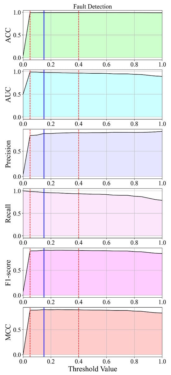
Figure 18.
The TBVE for fault detection based on multiple TBVE models. The red dashed lines represent the range of highest classification performance (threshold values 0.05 and 0.4), while blue line indicates the highest classification performance (threshold value 0.15).
The TBVE based on the RFC for fault detection (Figure 18) has an optimal threshold value at 0.15 using whichever highest classification performance can be achieved. As the threshold value increases, the evaluation metric values decrease. This is valid for all evaluation metrics except for precision, i.e., the metric increases as the threshold value increases. The range with a high classification performance indicated with red dashed lines is wide and only works with threshold values lower than 0.4 and higher than 0.05.
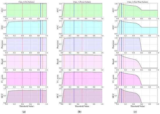
Figure 19.
The classification performance versus threshold values of TBVEs for Classes 0, 1, and 2. (a) The TBVE for detection of Class_0 (No Samples). Threshold range with high classification performance 0.4–0.95 (red dashed lines). Highest classification performance at threshold value 0.85. (b) The TBVE for detection of Class_1 (Power Failure). Threshold range with high classification performance 0.05–0.5 (red dashed lines). Highest classification performance at threshold value 0.3. (c) The TBVE for detection of Class_2 (Tool Wear Failure). Threshold range with high classification performance 0.05–0.15 (red dashed lines). Highest classification performance at threshold value 0.1.
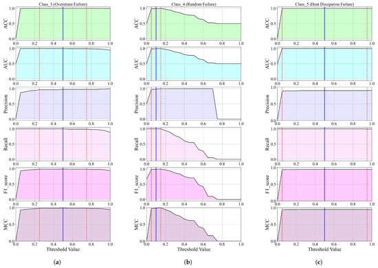
Figure 20.
The classification performance versus threshold values of TBVEs for Classes 3, 4, and 5. (a) The TBVE for detection of Class_3 (Overstrain Failure). Threshold range with high classification performance 0.25–0.75 (red dashed lines). Highest classification performance at threshold value 0.5. (b) The TBVE for detection of Class_4 (Random Failure). Threshold range with high classification performance 0.05–0.15 (red dashed lines). Highest classification performance at threshold value 0.1. (c) The TBVE for detection of Class_5 (Heat Dissipation Failure). Threshold range with high classification performance 0.1–0.95 (red dashed lines). Highest classification performance at threshold value 0.5.
The classification performance versus threshold value range of TBVEs for Classes 0, 1, and 2 shown in Figure 19 shows a different performance. The TBVE for Class_0 and 1 have a similar performance; however, the threshold range of high classification performance is larger in the case of Class_0 TBVE. It is interesting to notice that to detect Class_0, the threshold value must be higher than 0.4; however, to detect Class_1, the threshold value can be as low as 0.05. The TBVE for Class_2 has a very interesting classification performance. After the initial peak at a threshold value of 0.05, the classification performance tends to rapidly decrease. The Class_2 TBVE performance could be attributed to the low number of samples (45 in the initial dataset), which, with applications of oversampling techniques and later applications of the GPSC and the RFC, contributed to the overfitting.
As seen from Figure 20, the TBVEs for Class_3 and Class_5 have a similar performance, although the Class_5 TBVE has a wider threshold range with a higher classification performance. On the other hand, the Class_4 TBVE has a smaller threshold range where the TBVE achieves a higher classification performance. In the case of the Class_4 TBVE, as the threshold value increases from 0.15 to 1.0, the classification performance decreases.
4. Discussion
The dataset used in this research consists of 10,000 samples, 10 input variables (features), and two target variables (target—failure or not and Failure Type—type of failure). Some features had to be removed since they do not contribute in ML modeling to the prediction of the target variable and could lead to potential overfitting, i.e., unique identifier (UID) and product ID. The other variables are air temperature, process temperature, rotational speed, torque, and tool wear.
The target variable "Target" was used in this research for the detection of failure. This is a binary classification problem, and the "Target" variable in this form is already in numeric format, so the application of any preprocessing techniques such as Label Encoder was not required. The second variable was "Failure Type" and was used in the detection of Failure Type. There are six categories in this variable, and these are No Failure, Power Failure, Tool Wear Failure, Overstrain failure, Random Failure, and Heat Dissipation Failure. Using Label Encoder, these classes were transformed into 0 (No Failure), 1 (Power Failure), 2 (Tool Wear Failure), 3 (OverStrain Failure), 4 (Random Failure), and 5 (Heat Dissipation Failure).
The results shown in Figure 14 demonstrate that the SEs achieved a high classification performance across most balanced dataset variations, with SVMSMOTE consistently yielding the best results regardless of the scaler applied. Notably, the combination of MinMaxScaler and SVMSMOTE achieved the highest accuracy (0.9448), AUC (0.9449), and F1-score (0.9458), confirming the robustness of this pairing. BorderlineSMOTE also performed well, particularly with StandardScaler and RobustScaler, while ADASYN showed comparatively lower effectiveness. Interestingly, KMeansSMOTE consistently failed across all scalers, indicating incompatibility or issues with this resampling method in the current setup. Overall, this study highlights that the choice of oversampling technique and scaling method significantly impacts the performance of SE-based classifiers on balanced datasets.
The statistical analysis (Table 6) reveals that high-performing symbolic expressions were typically generated using larger populations, deeper trees, and dominant subtree mutation. Mutation rates like crossover, hoist, and point were minimal, while stopping criteria and parsimony pressure were rarely applied. The wide range of constants and variation in key parameters like population size and tree depth indicate that flexible and diverse hyperparameter settings are crucial for optimal GPSC performance across different balanced datasets.
The classification performance across balanced dataset variations demonstrates that symbolic expressions (SEs) combined with appropriate oversampling and scaling techniques achieve robust and reliable results for Classes 0, 1, and 2 (Figure 15).
For Class 0, the best outcomes were attained using SVMSMOTE paired with StandardScaler or RobustScaler, achieving accuracy and F1-scores above 0.93. PowerTransformer with BorderlineSMOTE also performed well, particularly in precision. In contrast, KMeansSMOTE consistently failed to generate valid models, indicating poor compatibility.
For Class 1, near-perfect classification metrics were observed, notably with the original unscaled KMeansSMOTE dataset and PowerTransformer combined with SVMSMOTE, both exceeding 0.99 in accuracy and F1-score. BorderlineSMOTE with RobustScaler and StandardScaler also produced highly robust results. Similar to Class 0, KMeansSMOTE generally underperformed except in its original form.
For Class 2, BorderlineSMOTE combined with StandardScaler, RobustScaler, or PowerTransformer yielded the highest accuracy and F1-scores (0.98), highlighting its reliability. SVMSMOTE paired with MinMaxScaler or PowerTransformer also showed a strong performance. Again, KMeansSMOTE variations failed consistently.
Overall, BorderlineSMOTE and SVMSMOTE, when combined with effective scaling methods like StandardScaler, RobustScaler, and PowerTransformer, consistently outperformed other oversampling techniques across these classes. These findings underscore the importance of selecting compatible oversampling-scaling pairs to maximize the effectiveness of SE-based classifiers on imbalanced datasets.
The optimal GPSC hyperparameters across all classes reveal a consistent pattern of relatively large population sizes (around 580 to 660) and moderate numbers of generations (approximately 56 to 65), both with notable variability. Tournament sizes are substantial, typically between 275 and 315, supporting strong selective pressure. Initialization depths span similar ranges (around 3.8–4 lower bound to 11.5–12.3 upper bound), suggesting a balanced initial complexity of symbolic expressions.
Crossover rates remain uniformly low (roughly 0.008 to 0.013), while subtree mutation rates are consistently high (around 0.71 to 0.80), highlighting a mutation-driven evolutionary search strategy. Hoist and point mutation rates are kept minimal but present (0.007 to 0.011), contributing subtle variation without destabilizing convergence.
The stopping criteria are very small (0.0003 to 0.0005), indicating stringent termination conditions. Maximum sample usage is generally high (0.74 to 0.82), ensuring broad data exposure during evolution. Constant ranges vary widely across classes but maintain a consistent, broad search space for numeric constants. Lastly, parsimony coefficients are uniformly low (0.00035 to 0.00041), reflecting a controlled penalty on model complexity.
Overall, these hyperparameter settings reflect a well-balanced evolutionary approach, emphasizing mutation over crossover, large, diverse populations, and careful control over complexity, leading to effective and robust symbolic classifiers for all classes.
Unfortunately, the TBVEs based on SEs were unstable and did not generate satisfactory results. Instead, the outputs for the SEs of each class were used to create the meta-datasets. These datasets were subjected again to preprocessing and oversampling, and the Random Forest Classifier (RFC) was trained on each dataset using RandomizedSearchCV with 5FCV. The best models with optimal hyperparameters were saved, and using the saved models, the TBVE for each class was created. The TBVEs for
- Fault detection (Figure 18) generated a perfect classification performance for threshold values equal to 0.15 or higher.
- Fault classification Class_0 (Figure 19a) generated a perfect classification performance for threshold values equal to 0.85 or higher.
- Fault classification Class_1 (Figure 19b) generated a perfect classification performance for threshold values equal to 0.3 or higher.
- Fault classification Class_2 (Figure 19c) generated a near-perfect classification performance for threshold values equal to 0.1 or higher.
- Fault classification Class_3 (Figure 20a) generated a near-perfect classification performance for threshold values equal to 0.5 or higher.
- Fault classification Class_4 (Figure 20b) generated a near-perfect classification performance for threshold values equal to 0.1 or higher.
- Fault classification Class_5 (Figure 20c) generated a near-perfect classification performance for threshold values equal to 0.5 or higher.
When compared to results reported in other recent studies summarized in Table 1, the proposed method—particularly the Threshold-Based Voting Ensemble (TBVE) constructed from Random Forest Classifiers (RFCs) trained on meta-datasets derived from symbolic expressions—demonstrated a perfect classification performance in both fault detection and fault classification tasks. This level of performance is competitive with or exceeds existing approaches in the literature.
For example, in [11], a hybrid model combining genetic algorithms (GAs) with Artificial Neural Networks (ANNs) achieved perfect classification accuracy for bearing fault diagnosis. Similarly, in [12], fault classification using ANNs also reached 100% accuracy on their selected dataset. While these results are strong in terms of raw performance, they rely on black-box neural networks, which do not provide interpretable decision logic and thus limit trust and diagnostic insight in real-world deployments.
In contrast, the proposed approach retains a high predictive performance while introducing interpretability through SEs obtained via the GPSC. These SEs are transparent mathematical formulas, which provide domain experts with a clear understanding of the relationships between sensor features and predicted failure modes. This is a significant advantage in the context of predictive maintenance, where model decisions must often be verified by engineers, and compliance or certification may require transparent logic.
Furthermore, the ensemble strategy—which uses SEs as meta-features for training robust RFC models and then combines them through threshold-based voting—offers stability, scalability, and generalization. This hierarchical architecture allows the system to recover from the limitations of individual SEs and produce consistently high-performing results across imbalanced datasets.
In summary, the key advantages of the proposed approach over works such as [11,12] include the following:
- Inherent interpretability, enabling deeper insight into fault mechanisms;
- High classification accuracy, comparable or superior to existing black-box models;
- Robustness to imbalanced data, achieved through systematic oversampling and one-vs-rest decomposition;
- Modular ensemble design, which can be tuned and extended for real-time monitoring and incremental learning.These features make the proposed method well-suited for industrial adoption, where both performance and explainability are essential.
5. Conclusions
In this paper, the publicly available dataset was used for machine predictive maintenance. The GPSC was applied to the dataset to obtain the SEs that could detect and classify the machine failure with high classification performance. The initial dataset investigation and statistical analysis showed that dataset variables have different ranges and that the dataset target class is highly imbalanced. Using the one-versus-rest approach from the initial multi-class dataset, several binary datasets were created. Using different preprocessing and oversampling techniques, a large number of balanced dataset variations were created for each class. The GPSC was trained using 5FCV, and the optimal combination of hyperparameters was found using the RHVS method. After the best SEs were obtained, the TBVE was developed; however, using this approach did not generate satisfactory results, i.e., the classification performance was not improved when compared to the individual SEs. The SEs were used to obtain the output, thus creating the meta-dataset which was imbalanced, so the scaling/normalization and oversampling techniques were used, and the RFC was trained on each balanced dataset variation using RandomizedSearchCV. The best RFC models were combined for each class, thus creating the TBVE, and the optimal threshold values were found for each TBVE using whichever classification performance was improved. Based on the conducted investigation, the conclusions are as follows:
- The GPSC generated SEs with a high classification performance in machine failure.
- The data scaling/normalization techniques and oversampling techniques generated a large number of dataset balancing techniques. Using these techniques introduced a large number of dataset variations that in the end generated a large number of SEs with a high classification performance.
- The 5FCV training process of the GPSC generated a large number of SEs. Using this training process created a robust set of SEs with a high classification performance.
- The RHVS method proved useful in finding an optimal combination of GPSC hyperparameters using whichever obtained set of SEs had a high classification performance.
- The combination of SEs failed to produce a TBVE with a stable performance. However, a dataset created from the outputs of SEs provides a meta-dataset used for training the RFCs. The TBVEs based on the RFCs generated a stable performance with high classification accuracy.
The advantages of using the proposed methodology are as follows:
- Unlike ANNs or other deep learning methods, the GPSC generates SEs that can be explainable, which are easier to handle and process.
- The application of preprocessing and oversampling techniques generated a large number of balanced dataset variations. Using this approach, the balanced datasets have synthetic data based on the statistics of the original dataset.
- The RHVS method generally finds the optimal combination of GPSC hyperparameter values very quickly when compared to grid search methods.
- The TBVE based on the RFC proved to be a very useful approach in creating a robust system with a high classification performance with the adjustment of threshold values.
While the proposed hybrid methodology demonstrated a strong classification performance and explainability, several disadvantages (limitations) remain:
- The GPSC training is computationally expensive, especially with large population sizes, many generations, and multiple balanced dataset variations created by preprocessing and oversampling.
- The Random Hyperparameter Value Search (RHVS) method, although effective, sometimes requires many GPSC runs to meet performance thresholds, which can further increase training time.
- The method’s performance is lower on classes with extremely limited samples, indicating challenges in handling highly imbalanced or rare Failure Types.
To address these limitations and enhance practical applicability, future research will explore the following:
- Reducing GPSC complexity by tuning population size and generation count to balance performance and runtime.
- Investigating alternative hyperparameter optimization techniques such as Bayesian optimization to improve efficiency over RHVS.
- Developing advanced oversampling or data augmentation methods tailored to minority classes with very few samples to boost detection accuracy.
- Applying model pruning or distillation methods to simplify symbolic expressions and ensemble models for faster inference.
- Testing the framework on larger and more diverse real-world predictive maintenance datasets to validate scalability and robustness.
Author Contributions
Conceptualization, N.A. and S.B.Š.; methodology, N.A.; software, N.A.; validation, N.A., S.B.Š. and V.M.; formal analysis, N.A.; investigation, N.A.; resources, N.A.; data curation, N.A.; writing—original draft preparation, N.A. and S.B.Š.; writing—review and editing, N.A.; visualization, N.A.; supervision, N.A. and V.M.; project administration, N.A.; funding acquisition, S.B.Š. All authors have read and agreed to the published version of the manuscript.
Funding
This research received no external funding.
Data Availability Statement
The dataset used in this research is a publicly available dataset from Kaggle https://www.kaggle.com/datasets/shivamb/machine-predictive-maintenance-classification (accessed on 19 February 2025).
Conflicts of Interest
The authors declare no conflicts of interest.
Appendix A. The Modified Mathematical Functions Used in GPSC
As stated in the description of the GPSC, some mathematical functions such as division, square root, natural logarithm, and logarithms with bases 2 and 10 had to be modified to avoid generating infinity values, non-number values, or imaginary values which could lead to early termination of the GPSC without generating SEs. The modified division function can be written as
The and variables do not have any connection with the input variables of the dataset used in this research. They are used here for the definition of the modified division function. The modified square root function is defined as
The natural logarithm and logarithms with bases 2 and 10 are defined as
where i represents the bases of logarithm e for natural logarithm, 2 for logarithm with base 2, and 10 for logarithm with base 10.
Appendix B. Where to Find SEs Obtained in This Research and How to Use Them
All the SEs obtained in this research for fault detection and classification can be download from the GitHub repository https://github.com/nandelic2022/Predictive_Maintenace.git (accessed on 2 July 2025). To use these SEs on a new dataset, make sure that the dataset has the same number of input variables and in the same order as in the dataset used in this research. If SEs were used that were obtained on the dataset preprocessed with any scaler/normalizer, then the dataset values have to be preprocessed with the same scaler/normalizer.
To obtain the class value from the SEs, first, the values of the input variables must be provided for the SE. After the value is obtained, then the class is determined through the Sigmoid function, where the input in the Sigmoid function is the output of the SE.
References
- Molęda, M.; Małysiak-Mrozek, B.; Ding, W.; Sunderam, V.; Mrozek, D. From corrective to predictive maintenance—A review of maintenance approaches for the power industry. Sensors 2023, 23, 5970. [Google Scholar] [CrossRef] [PubMed]
- Lee, J.; Ni, J.; Singh, J.; Jiang, B.; Azamfar, M.; Feng, J. Intelligent maintenance systems and predictive manufacturing. J. Manuf. Sci. Eng. 2020, 142, 110805. [Google Scholar] [CrossRef]
- Yazdi, M. Maintenance strategies and optimization techniques. In Advances in Computational Mathematics for Industrial System Reliability and Maintainability; Springer: Berlin/Heidelberg, Germany, 2024; pp. 43–58. [Google Scholar]
- Uptime Institute. Global Data Center Survey, 2022. Available online: https://uptimeinstitute.com (accessed on 2 July 2025).
- Deloitte. Predictive Maintenance: Next-Generation Maintenance Strategy. 2017. Available online: https://www2.deloitte.com (accessed on 2 July 2025).
- Shah, A.; Kumar, R.; Jain, V. Forecasting Remaining Useful Life for Wind Turbine Predictive Maintenance Based on Deep Learning. arXiv 2024, arXiv:2412.17823. [Google Scholar]
- Al Hasib, A.; Islam, M.; Chowdhury, M. An Interpretable Systematic Review of Machine Learning Models for Predictive Maintenance of Aircraft Engines. arXiv 2023, arXiv:2309.13310. [Google Scholar]
- Carvalho, T.P.; Soares, F.A.; Vita, R.; Francisco, R.d.P.; Basto, J.P.; Alcalá, S.G. A systematic literature review of machine learning methods applied to predictive maintenance. Comput. Ind. Eng. 2019, 137, 106024. [Google Scholar] [CrossRef]
- Vuttipittayamongkol, P.; Arreeras, T. Data-driven industrial machine failure detection in imbalanced environments. In Proceedings of the 2022 IEEE International Conference on Industrial Engineering and Engineering Management (IEEM), Kuala Lumpur, Malaysia, 7–10 December 2022; IEEE: Piscataway, NJ, USA, 2022; pp. 1224–1227. [Google Scholar]
- Luo, B.; Wang, H.; Liu, H.; Li, B.; Peng, F. Early fault detection of machine tools based on deep learning and dynamic identification. IEEE Trans. Ind. Electron. 2018, 66, 509–518. [Google Scholar] [CrossRef]
- Samanta, B.; Al-Balushi, K.R.; Al-Araimi, S.A. Bearing fault detection using artificial neural networks and genetic algorithm. EURASIP J. Adv. Signal Process. 2004, 2004, 785672. [Google Scholar] [CrossRef]
- Leh, N.A.M.; Zain, F.M.; Muhammad, Z.; Abd Hamid, S.; Rosli, A.D. Fault detection method using ANN for power transmission line. In Proceedings of the 2020 10th IEEE International Conference on Control System, Computing and Engineering (ICCSCE), Penang, Malaysia, 21–22 August 2020; IEEE: Piscataway, NJ, USA, 2020; pp. 79–84. [Google Scholar]
- Mesai Belgacem, A.; Hadef, M.; Djerdir, A. Fault diagnosis of photovoltaic array based on gated residual network with multi-head self attention mechanism. Turk. J. Electr. Eng. Comput. Sci. 2024, 32, 806–828. [Google Scholar] [CrossRef]
- Apeiranthitis, S.; Zacharia, P.; Chatzopoulos, A.; Papoutsidakis, M. Predictive maintenance of machinery with rotating parts using Convolutional Neural Networks. Electronics 2024, 13, 460. [Google Scholar] [CrossRef]
- Pantelis, L.; Papastefanopoulos, V.; Kotsiantis, S. Explainable ai: A review of machine learning interpretability methods. Entropy 2023, 23, 18. [Google Scholar]
- Dereci, U.; Tuzkaya, G. An explainable artificial intelligence model for predictive maintenance and spare parts optimization. Supply Chain Anal. 2024, 8, 100078. [Google Scholar] [CrossRef]
- Kramer, O.; Kramer, O. Scikit-learn. In Machine Learning for Evolution Strategies; Springer: Berlin/Heidelberg, Germany, 2016; pp. 45–53. [Google Scholar]
- Fernández, A.; Garcia, S.; Herrera, F.; Chawla, N.V. SMOTE for learning from imbalanced data: Progress and challenges, marking the 15-year anniversary. J. Artif. Intell. Res. 2018, 61, 863–905. [Google Scholar] [CrossRef]
- He, H.; Bai, Y.; Garcia, E.A.; Li, S. ADASYN: Adaptive synthetic sampling approach for imbalanced learning. In Proceedings of the 2008 IEEE International Joint Conference on Neural Networks (IEEE World Congress on Computational Intelligence), Hong Kong, China, 1–6 June 2008; IEEE: Piscataway, NJ, USA, 2008; pp. 1322–1328. [Google Scholar]
- Han, H.; Wang, W.Y.; Mao, B.H. Borderline-SMOTE: A new over-sampling method in imbalanced data sets learning. In Proceedings of the International Conference on Intelligent Computing, Hefei, China, 23–26 August 2005; Springer: Berlin/Heidelberg, Germany, 2005; pp. 878–887. [Google Scholar]
- Fonseca, J.; Douzas, G.; Bacao, F. Improving imbalanced land cover classification with K-Means SMOTE: Detecting and oversampling distinctive minority spectral signatures. Information 2021, 12, 266. [Google Scholar] [CrossRef]
- Bagui, S.S.; Mink, D.; Bagui, S.C.; Subramaniam, S. Determining Resampling Ratios Using BSMOTE and SVM-SMOTE for Identifying Rare Attacks in Imbalanced Cybersecurity Data. Computers 2023, 12, 204. [Google Scholar] [CrossRef]
- Langdon, W.B.; Poli, R. Foundations of Genetic Programming; Springer Science & Business Media: Berlin/Heidelberg, Germany, 2013. [Google Scholar]
- O’Neill, M.; Poli, R.; Langdon, W.B.; McPhee, N.F. A Field Guide to Genetic Programming; Springer: Berlin/Heidelberg, Germany, 2008; 250p, ISBN 978-1-4092-0073-4. [Google Scholar]
- Kyurkchiev, N.; Markov, S. Sigmoid functions: Some approximation and modelling aspects. LAP LAMBERT Acad. Publ. Saarbr. 2015, 4, 34. [Google Scholar]
- Hurtik, P.; Tomasiello, S.; Hula, J.; Hynar, D. Binary cross-entropy with dynamical clipping. Neural Comput. Appl. 2022, 34, 12029–12041. [Google Scholar] [CrossRef]
- Ben-David, A.; Frank, E. Accuracy of machine learning models versus “hand crafted” expert systems–a credit scoring case study. Expert Syst. Appl. 2009, 36, 5264–5271. [Google Scholar] [CrossRef]
- De Hond, A.A.; Steyerberg, E.W.; Van Calster, B. Interpreting area under the receiver operating characteristic curve. Lancet Digit. Health 2022, 4, e853–e855. [Google Scholar] [CrossRef] [PubMed]
- Zhou, Q.M.; Zhe, L.; Brooke, R.J.; Hudson, M.M.; Yuan, Y. A relationship between the incremental values of area under the ROC curve and of area under the precision-recall curve. Diagn. Progn. Res. 2021, 5, 1–15. [Google Scholar] [CrossRef] [PubMed]
- Yacouby, R.; Axman, D. Probabilistic extension of precision, recall, and f1 score for more thorough evaluation of classification models. In Proceedings of the First Workshop on Evaluation and Comparison of NLP Systems, Online, 20 November 2020; pp. 79–91. [Google Scholar]
- Visa, S.; Ramsay, B.; Ralescu, A.L.; Van Der Knaap, E. Confusion matrix-based feature selection. Maics 2011, 710, 120–127. [Google Scholar]
Disclaimer/Publisher’s Note: The statements, opinions and data contained in all publications are solely those of the individual author(s) and contributor(s) and not of MDPI and/or the editor(s). MDPI and/or the editor(s) disclaim responsibility for any injury to people or property resulting from any ideas, methods, instructions or products referred to in the content. |
© 2025 by the authors. Licensee MDPI, Basel, Switzerland. This article is an open access article distributed under the terms and conditions of the Creative Commons Attribution (CC BY) license (https://creativecommons.org/licenses/by/4.0/).