Article

Innovative Flow Pattern Identification in Oil–Water Two-Phase Flow via Kolmogorov–Arnold Networks: A Comparative Study with MLP

1
College of Geophysics and Petroleum Resources, Yangtze University, Wuhan 430100, China
2
Key Laboratory of Exploration Technologies for Oil and Gas Resources, Yangtze University, Ministry of Education, Wuhan 430100, China
*
Author to whom correspondence should be addressed.
Processes 2025, 13(8), 2562; https://doi.org/10.3390/pr13082562
Submission received: 17 July 2025 / Revised: 11 August 2025 / Accepted: 12 August 2025 / Published: 14 August 2025
(This article belongs to the Section Energy Systems)

Abstract

As information and sensor technologies advance swiftly, data-driven approaches have emerged as a dominant paradigm in scientific research. In the petroleum industry, precise forecasting of patterns of two-phase flow involving oil and water is essential for enhancing production efficiency and ensuring safety. This study investigates the application of Kolmogorov–Arnold Networks (KAN) for predicting patterns of two-phase flow involving oil and water and compares it with the conventional Multi-Layer Perceptron (MLP) neural network. To obtain real physical data, we conducted the experimental section to simulate the patterns of two-phase flow involving oil and water under various well angles, flow rates, and water cuts at the Key Laboratory of Oil and Gas Resources Exploration Technology of the Ministry of Education, Yangtze University. These data were standardized and used to train both KAN and MLP models. The findings indicate that KAN outperforms the MLP network, achieving 50% faster convergence and 22.2% higher accuracy in prediction. Moreover, the KAN model features a more streamlined structure and requires fewer neurons to attain comparable or superior performance to MLP. This research offers a highly effective and dependable method for predicting patterns of two-phase flow involving oil and water in the dynamic monitoring of production wells. It highlights the potential of KAN to boost the performance of energy systems, particularly in the context of intelligent transformation.

1. Introduction

The rapid advancement of information and communication technologies, coupled with the proliferation of connected devices and sensor networks, has resulted in an unprecedented surge of data in numerous fields. This includes critical sectors such as financial services [1,2], the oil and gas industry [3,4], and digital communication platforms [5]. These extensive datasets encapsulate the intricate spatiotemporal characteristics of operational processes, thereby providing valuable insights and strategic opportunities to optimize efficiency [6,7,8,9]. The concurrent increase in computational capabilities, improvements in hardware technology, enhanced data literacy, and the evolution of sophisticated data-driven modeling techniques have collectively fueled the explosive growth of data-centric research endeavors [10,11,12]. Such research has proven instrumental in enhancing performance and advancing the comprehension of exploration, development, and production optimization within the petroleum sector [13,14,15,16]. As data-driven methodologies permeate various disciplines, we are witnessing the emergence of a new era in scientific inquiry—often termed the “data-centric scientific paradigm.” In this paradigm, data serves as the primary basis for decision-making, distinct from the conventional reliance on computational simulations or theoretical frameworks that are strictly grounded in physical laws [17].
The initial triumphs in data-driven methodologies largely relied on multi-layer feedforward neural architectures, particularly MLPs. Researchers have long recognized MLPs for their capacity to approximate complex functions, a capability supported by the universal approximation theorem [18,19]. Although MLPs excel at establishing nonlinear relationships within high-dimensional spaces, they face notable challenges. These include susceptibility to local minima, overfitting, and a “black-box” characteristic complicating interpretability. Historically, researchers often disregarded the black-box nature of MLPs due to their strong predictive performance. However, as the need for model transparency and the ability to trace causal relationships in predictive tasks has grown, the scientific community has increasingly focused on the interpretability of MLPs [20].
Addressing the limitations of MLPs in applications where transparency and interpretability are crucial, researchers have proposed KANs as a promising alternative [21]. Grounded in the Kolmogorov–Arnold theorem, which asserts that any multivariate function can be decomposed into the sum of univariate functions, KANs provide a new framework for interpreting the complex nonlinear relationships in neural networks. This theorem enables the decomposing of intricate multivariate functions into simpler, more interpretable components. KANs have shown modeling accuracy comparable to or exceeds that of MLPs while offering enhanced interpretability. However, the comparative performance of KANs and MLPs in various practical applications, such as image recognition, text processing, solving differential equations, predicting time-series data, simulating fluid dynamics, and monitoring the dynamic behavior of production wells in the petroleum industry, remains an ongoing topic of discussion [22,23,24,25,26].
In the petroleum industry, multiphase flow phenomena are encountered throughout the entire oil and gas exploration, production, and transportation lifecycle [27]. Among these, patterns of two-phase flow involving oil and water is particularly prevalent and significantly influences the efficiency of offshore oil field development, the safety of production equipment, and overall economic benefits. For example, in non-vertical wells, such as deviated and horizontal wells, the fluid within the wellbore is influenced by multiple physical forces, including gravity, centrifugal force, and wall friction. These forces form complex and dynamic flow patterns, such as stratified, slug, and dispersed flows. With the expansion of offshore oil field development, the prevalence of non-vertical wells has increased. However, these wells face several production challenges. Variations in flow patterns can cause production fluctuations and reduce efficiency. The complex flow conditions can also lead to pipeline corrosion and instrument failure, which increase maintenance costs and cause production delays, ultimately harming economic benefits. Consequently, the development of accurate, reliable, and interpretable methods for flow pattern recognition has become a critical requirement for the advancement of petroleum engineering [28].
Addressing the aforementioned technical challenges and research opportunities, this study systematically compares the performance of KANs and MLPs in fluid pattern prediction. Utilizing a multidimensional evaluation framework that includes (1) model training efficiency and (2) prediction accuracy (assessed through confusion matrix analysis of prediction results across various categories), empirical results demonstrate that KAN models maintain comparable prediction accuracy while reducing training steps by approximately 50%. This represents a significant improvement over traditional MLP architectures. These findings provide an interpretable and efficient modeling tool for dynamic optimization decision-making in the energy extraction sector, offering substantial engineering application value.
This research is laid out as follows: in Section 2, we explore the details of how KAN and MLP work. Section 3 details the experimental methodology employed in the study. Section 4 examines how we trained the networks. In Section 5, we break down how KAN and MLP compare. Finally, we wrap things up with some closing thoughts.

2. Method

2.1. Multi-Layer Perceptron

The Multi-Layer Perceptron (MLP) is a classic feedforward artificial neural network and fundamental architecture for deep learning. Mathematically, an MLP with L hidden layers maps an input vector x R n to an output y R m through a series of nonlinear transformations applied layer by layer.
The architecture of an MLP network comprises three main components: the input layer, hidden layers, and the output layer. The input layer functions to accept the initial input x . Each hidden layer l ( l = 1,2 , , L ) carries out the subsequent operations:
h ( l ) = σ ( W ( l ) h ( l 1 ) + b ( l ) )
Here, h ( l 1 ) R d l 1 represents the output from the previous layer ( h 0 = x ) , W ( l ) R d l × d l 1 and b ( l ) R d l are the learnable weight matrix and bias vector, respectively, and σ ( · ) is a fixed nonlinear activation function (such as ReLU, Sigmoid).
The output layer generates the final prediction through a linear transformation:
y = W ( L + 1 ) h ( L ) + b ( L + 1 )
The Universal Approximation Theorem ensures that an MLP with at least one hidden layer and sufficient width can approximate any continuous function on a compact domain. However, the theorem does not provide an explicit method for constructing the network. Figure 1 illustrates an MLP network model with two hidden layers. For a more in-depth understanding of the MLP’s operation, refer to [29,30,31,32].

2.2. Kolmogorov–Arnold Network

The KAN is a new type of neural network architecture based on the Kolmogorov–Arnold representation theorem, which states that if f ( x ) is a continuous multivariate function defined on a bounded domain, then it can be expressed as a finite composition of continuous single-variable functions and the binary operation of addition.
The theorem of Kolmogorov–Arnold indicates that any continuous multivariate function f ( x ) C ( [ 0,1 ] n ) can be expressed as:
f ( x ) = q = 1 2 n + 1   Φ q ( p = 1 n   ψ q , p ( x p ) )
Here, ϕ q , p maps the interval [ 0,1 ] to R , and ψ q , p maps R to R . This representation suggests that addition is the fundamental multivariate operation, as other functions can be constructed by combining unary functions through summation.
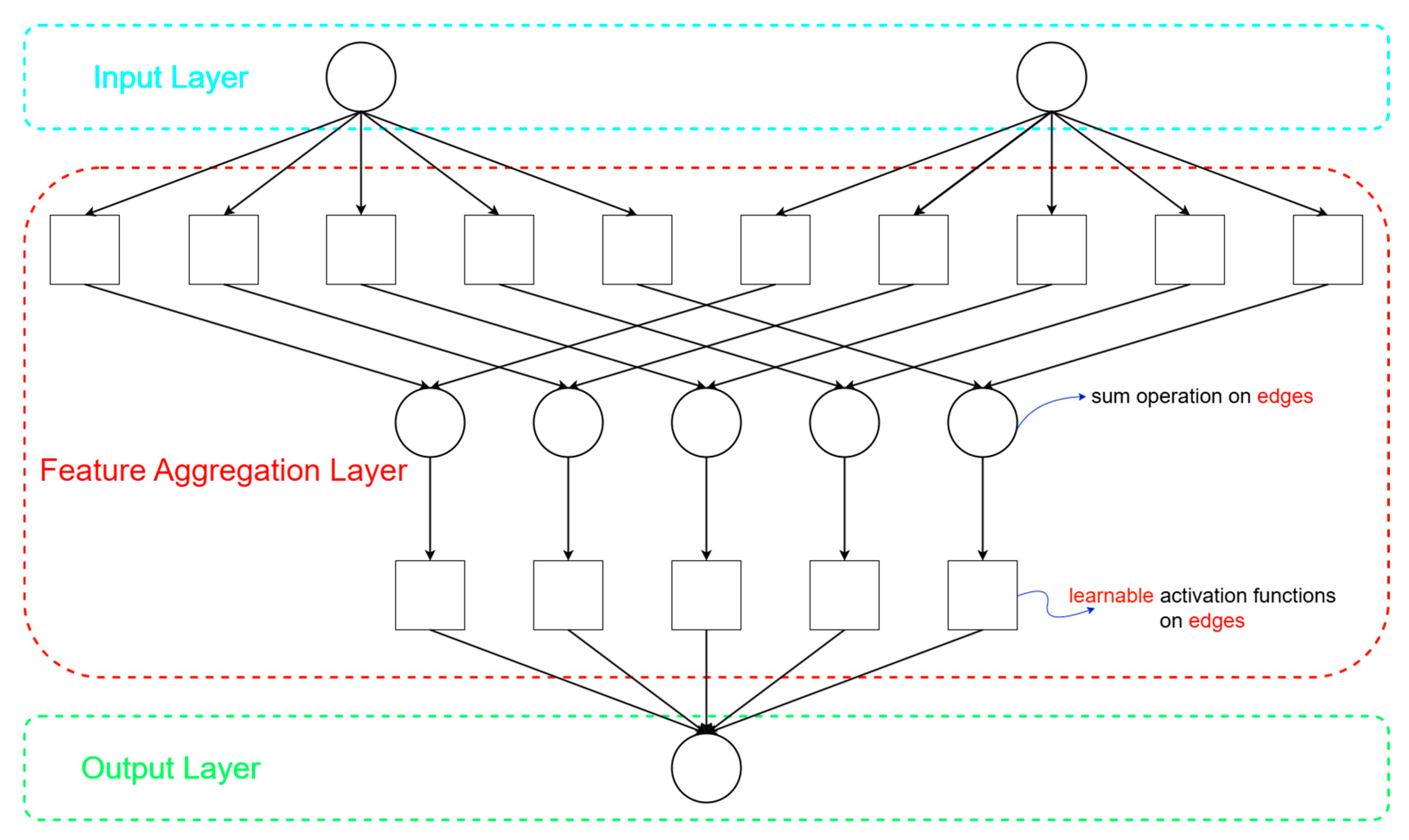
The architecture of KAN consists of three main layers: the input transformation layer, the feature aggregation layer, and the output synthesis layer. In the input transformation layer, each input variable x p is independently transformed through 2 n + 1 learnable univariate functions { ψ q , p ( x p ) } :
h q , p = ψ q , p ( x p ) , q = 1 , , 2 n + 1 ;   p = 1 , , n
The feature aggregation layer sums the transformed results along the input dimension to generate intermediate variables { z q } :
z q = p = 1 n   h q , p
The output synthesis layer synthesizes the final output through univariate functions { Φ q ( z q ) } :
y = q = 1 2 n + 1 Φ q ( z q )  
Like MLP, KAN employs a fully connected architecture. However, whereas MLP utilizes fixed activation functions at each node (“neurons”), KAN incorporates learnable activation functions on the edges (“weights”). Figure 2 depicts a standard three-layer KAN model. For a more in-depth understanding of the KAN’s operation, refer to [33,34,35].

3. Experimental Work

3.1. Experimental Device

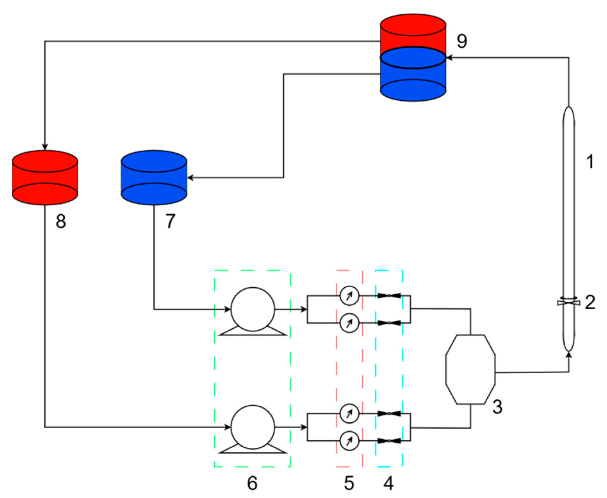
This study conducted experimental research on oil–water two-phase flow dynamics at the Multiphase Flow Laboratory of the Key Laboratory of Exploration Technologies for Oil and Gas Resources (Ministry of Education) at Yangtze University. Figure 3 illustrates the schematic diagram of the experimental setup. The main platform consists of a transparent cylindrical glass conduit with an inner diameter of 15.6 cm and a total length of 12 m, equipped with stainless steel observation sections (1 m each) at both ends for real-time recording of flow pattern dynamics. The experimental system integrates an oil–water mixing unit, a flow regulation module, and a data acquisition device. The oil phase is composed of No. 10 industrial white oil (density 0.8263 g/cm3, viscosity 2.92 mPa·s), while the water phase is tap water (density 0.9884 g/cm3, viscosity 1.16 mPa·s). The two phases are precisely proportioned through a mixer controlled by an electric ball valve.
The experimental platform is equipped with a Resistance Array Tool (RAT) and a Capacitance Array Tool (CAT), developed by Sondex Ltd. (Farnborough, UK), which are used to monitor the fluid’s electrical conductivity and dielectric constant distribution, respectively. The RAT captures real-time changes in the oil–water interface resistance through 12 bow-shaped spring sensors (see Figure 4). Based on circular capacitive measurement principles, the CAT analyzes the spatial distribution characteristics of different phases (see Figure 5). Data acquisition is set at a rate of 10 m/min and synchronized with high-speed camera recordings to obtain flow pattern images and physical parameters simultaneously.

3.2. Experimental Design

The experimental program encompasses four wellbore inclinations (0° vertical, 60° deviated, 85° near-horizontal, and 90° horizontal), three total flow rates (100, 300, and 600 m3/day), and five water cut levels (20%, 40%, 60%, 80%, and 90%). The experiments are conducted in a constant temperature environment (20 ± 1 °C) and under atmospheric pressure to replicate actual operating conditions. Each experimental run lasts 2 min, with data recorded after flow stabilization. A rapid valve-closure technique is employed to freeze the flow pattern, ensuring data representativeness instantaneously.
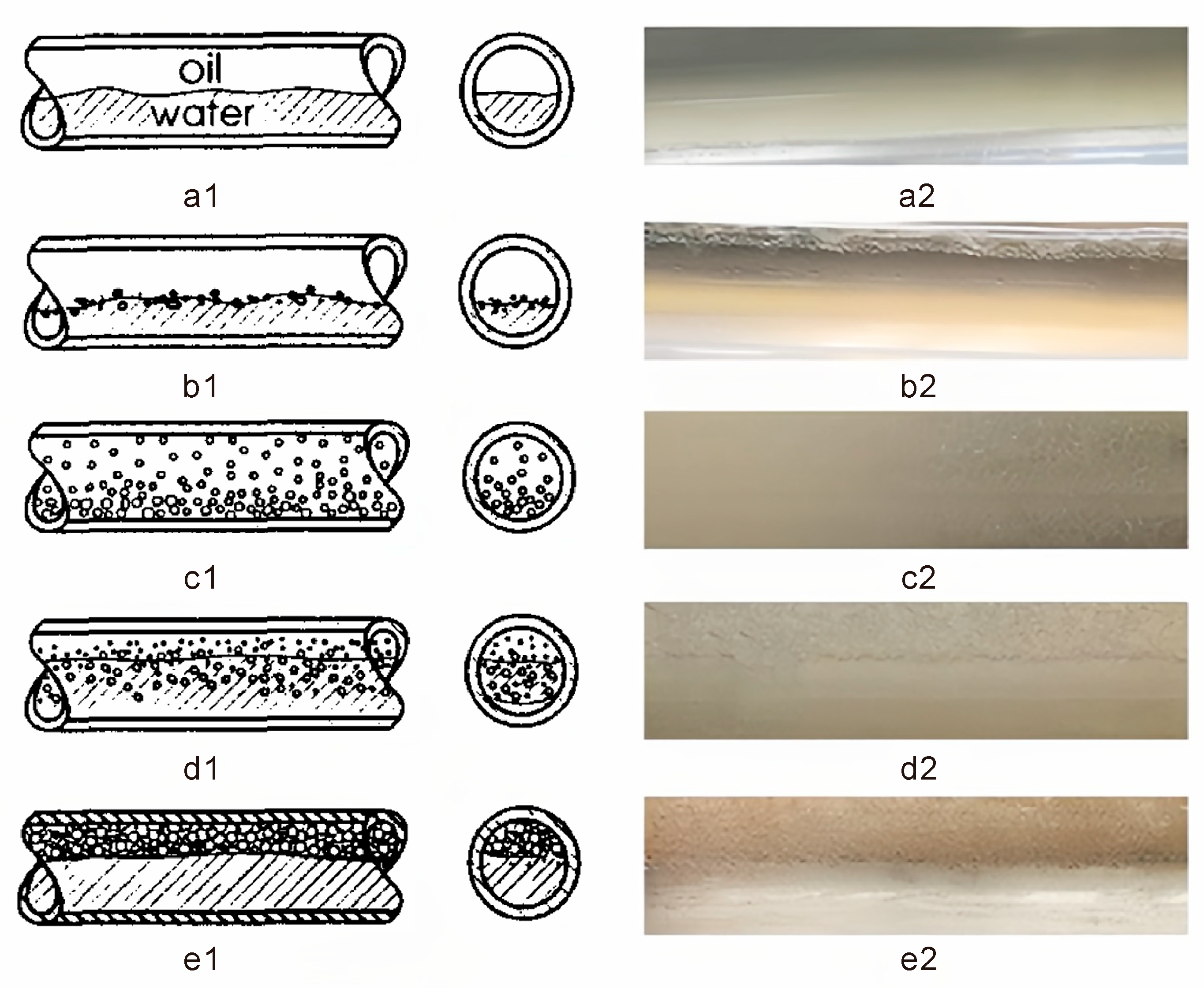
During the process, the original data were verified, and photos and videos were taken. Figure 6 presents the two-phase flow involving the oil and water pattern diagram (schematic source: literature [36]) and high camera records, which are as follows:
  • SS (a1,a2): The oil and water flow in distinct layers with a smooth interface.
  • ST & MI (b1,b2): The oil and water flow in layers, but there is some mixing at the interface.
  • W/O (c1,c2): The water is dispersed in the oil phase.
  • DW/O & O/W (d1,d2): The upper layer is water dispersed in oil, and the lower layer is oil with water droplets.
  • DO/W & W (e1,e2): The upper layer is oil dispersed in water, and the lower layer is water.

3.3. Experimental Data Processing

Upon completion of the experiment, to facilitate statistical analysis, the smooth stratified flow (SS) and the stratified flow with mixing at the interface (ST&MI) were merged into a single category termed stratified flow (ST). To effectively compare the MLP neural network’s and KAN’s prediction performance in identifying patterns of two-phase flow involving oil and water, a total of 60 experimental datasets were selected for this study. The well inclination angle, total flow rate, and water cut were utilized as features, while the flow pattern served as the label.
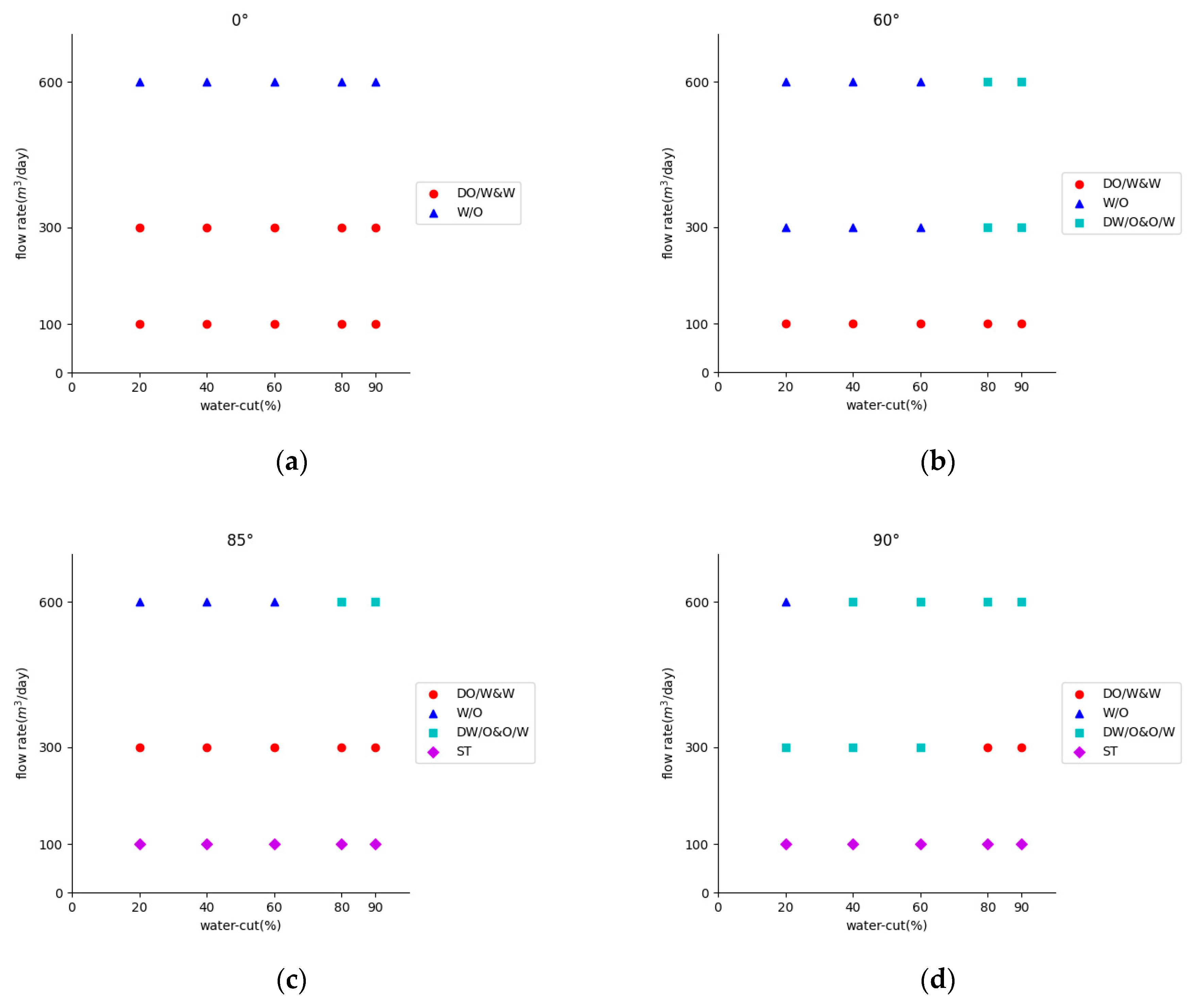
The experiment collected 60 valid datasets divided into training and testing sets in a 7:3 ratio. The sample data are depicted in Figure 7. The well inclination angle, total flow rate, and water cut were utilized as features, while the flow pattern served as the label. The input features included wellbore inclination, total flow rate, and water cut. Since neural networks cannot process non-numerical inputs during training, the four flow patterns were assigned target values, as detailed in Table 1. The data underwent standardization using the Z-score method to eliminate dimensional discrepancies. The formula for standardization is:
z = x μ σ
Here, x denotes the original data point, μ represents the mean of the data, and σ indicates the standard deviation of the data.

4. Network Training

4.1. Implementation Steps of MLP

Data preprocessing uses the MLP to predict patterns of two-phase flow involving oil and water. Subsequently, the MLP network is trained using the preprocessed data to optimize the training samples’ performance. The detailed implementation process is as follows:
Construct an MLP network with two hidden layers. Hidden layers 1 and 2 contain 12 and 6 neurons, respectively. The learning rate is manually adjusted to 0.001.
Proceed with the network training. Choose the suitable training function and training method. This study selects the ReLU activation function for the hidden layer and applies the softmax activation function to the output layer. The network uses the ‘model.fit()’ function in the Keras framework for model training, and then sparse_categorical_crossentropy is the loss function.
The data is accessible via the network, and the predicted value is subsequently derived.
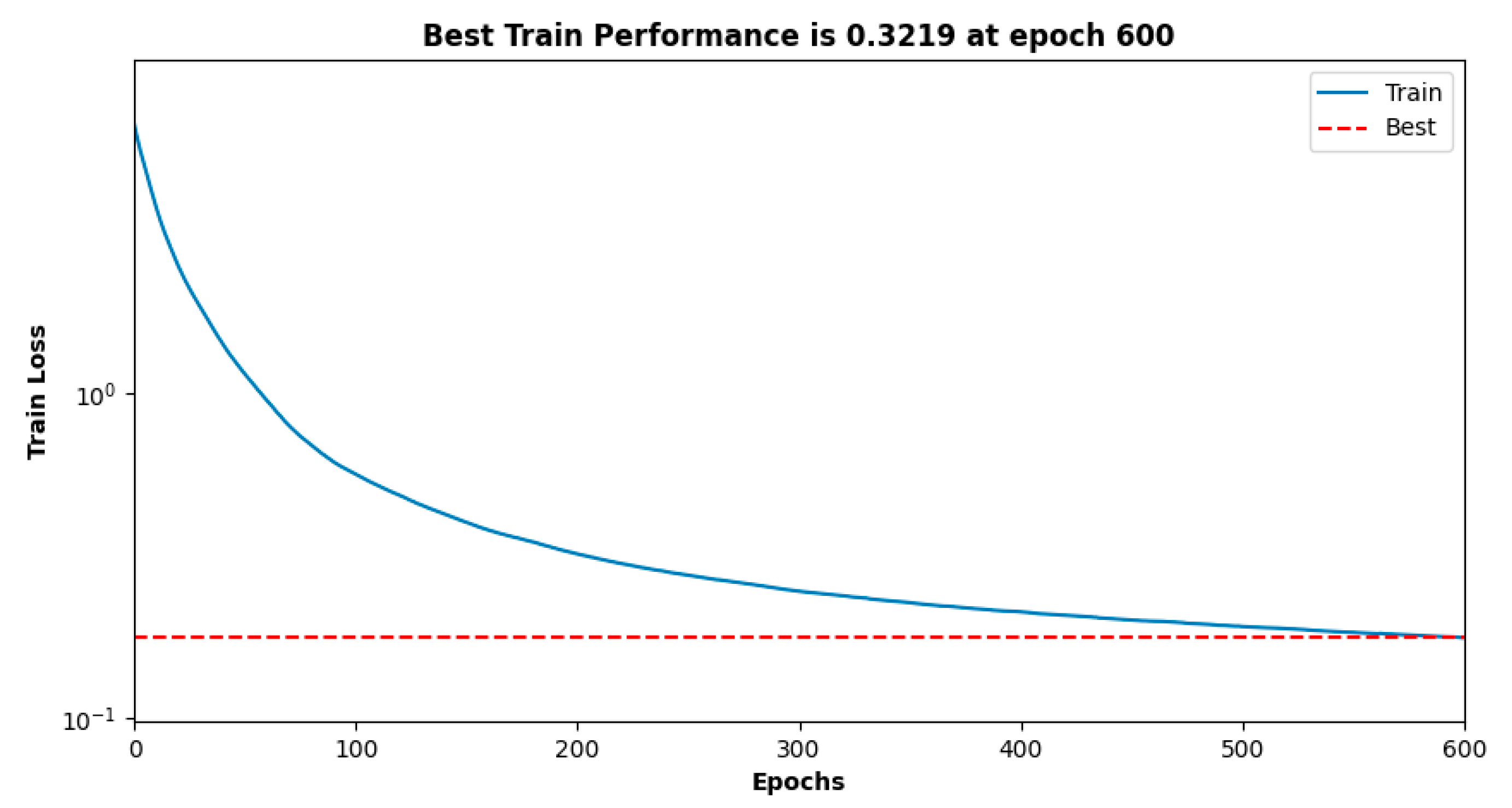
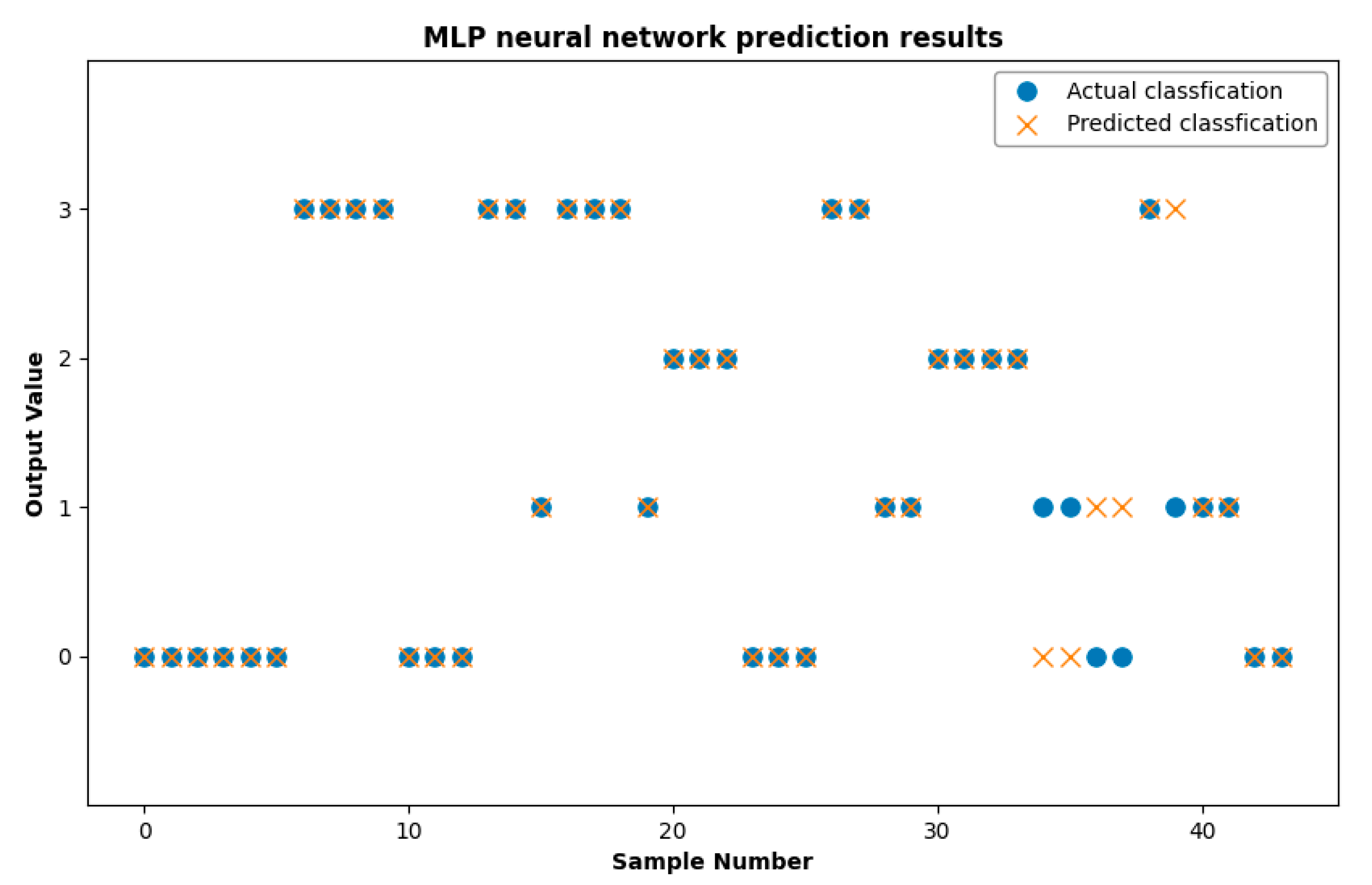
Figure 8 illustrates the training process. Upon reaching 600 training steps, the Train Loss converges. The prediction results obtained from the MLP neural network training consist of 42 sample datasets, as depicted in Figure 9. The solid blue circles represent the actual values, while the orange crosses denote the predicted values. The predicted values closely match the actual values, with only five incorrect predictions made by the MLP neural network in total.

4.2. Implementation Steps of KAN

When employing KAN to predict the patterns of two-phase flow involving oil and water, the same dataset as that used for the MLP neural network is selected, with 30% allocated as the test set. The detailed implementation process is as follows:
Construct a KAN with two hidden layers and set the number of training steps to 300, matching the configuration of the previously used MLP network. However, only seven neurons must be set per layer (2n + 1). Due to the characteristics of KAN, the learning rate is adjusted by the model itself, but it needs to give an initial value set to the same 0.001 as the MLP.
Continue to conduct network training. In KAN, the core implementation of the activation function is based on the B-spline basis function, and cubic B-splines are used in this study.
The data is accessible via the network, and the predicted value is subsequently derived.
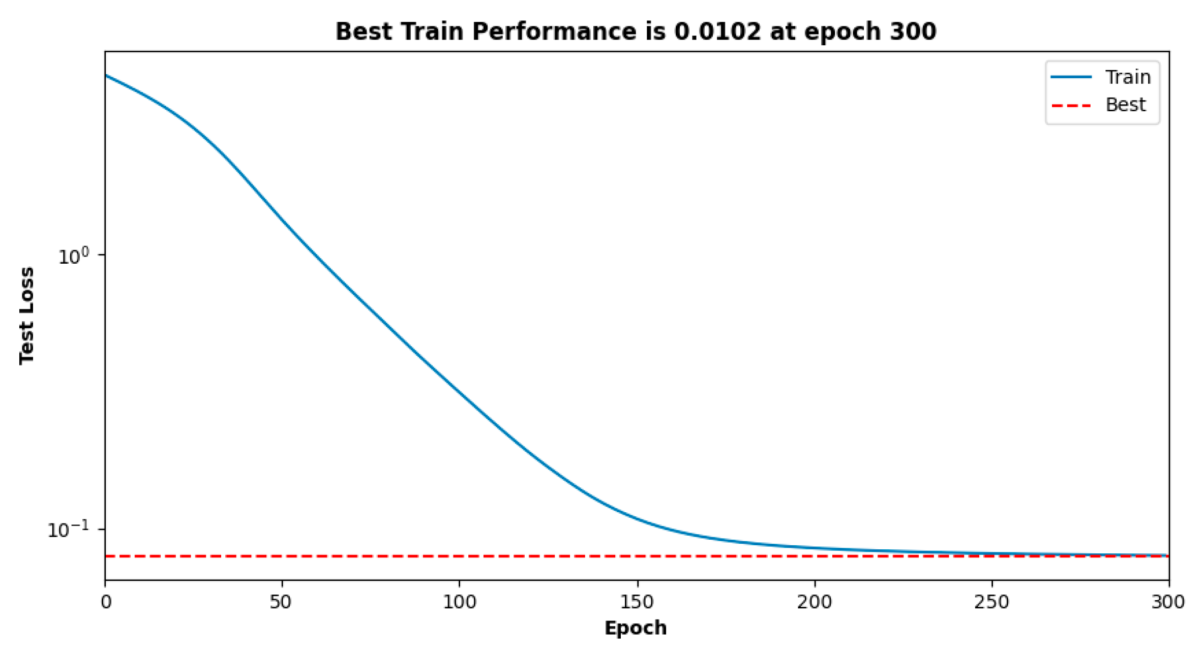
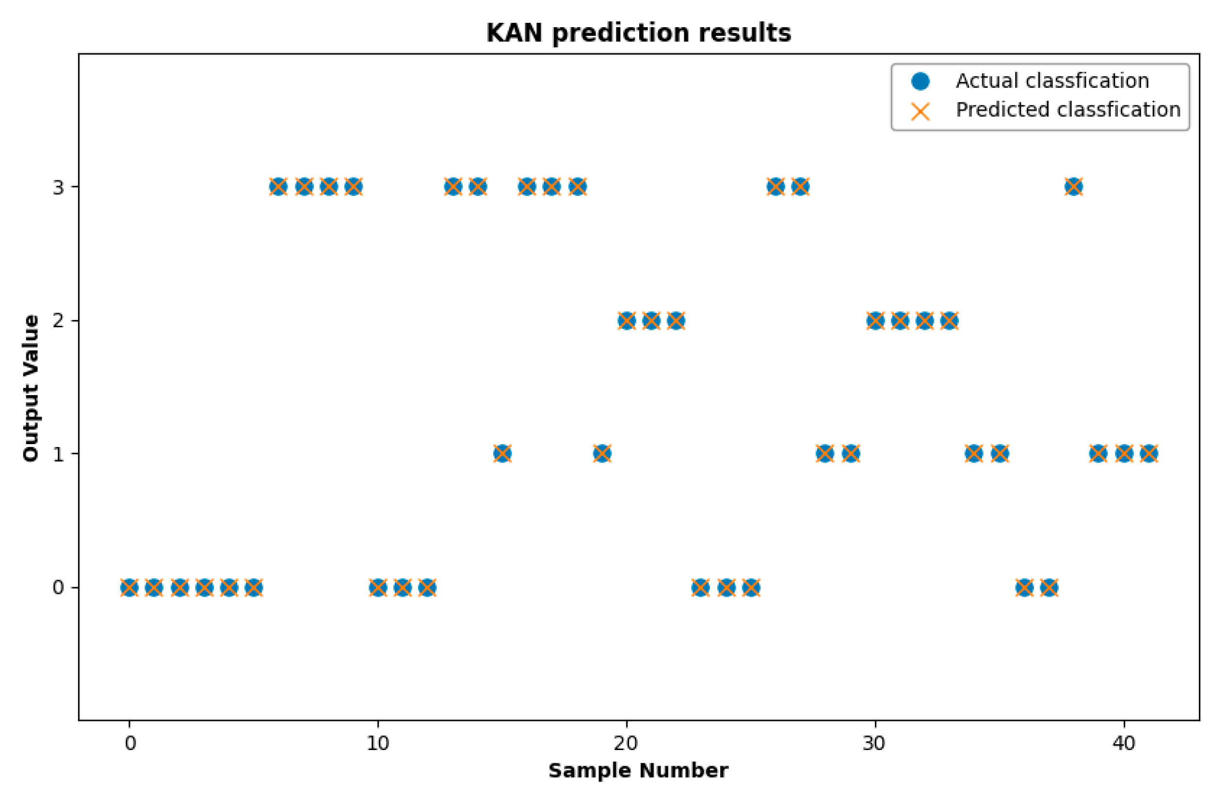
The training process is depicted in Figure 10. Upon reaching 300 training iterations, the Train Loss value stabilizes. Following the training of the KAN model, predictions were made for 42 sample datasets in the test set, with the results presented in Figure 11. The solid blue circles represent the actual values. At the same time, the orange crosses indicate the predicted values. The KAN model’s predictions align closely with the actual values when predicting the patterns of two-phase flow involving oil and water. Nevertheless, additional evaluation is necessary to determine the model’s accuracy in the test set.

5. Result & Discussion

This study employs the trained KAN model to align the prediction results more closely with actual production logging dynamic monitoring requirements to achieve more accurate predictions of the patterns of two-phase flow involving oil and water. During the experiment, analysis of the flow pattern diagrams for well inclinations of 0 degrees (vertical upward), 60 degrees (upward inclined), 85 degrees (upward inclined), and 90 degrees (horizontal) in Figure 7, revealed that the two-phase flow involving oil and water is influenced by three primary factors: inclination angle, flow rate, and water content. The outcomes of the KAN model are in agreement with the experimental findings.

Comparison of the KAN Model with the MLP Neural Network

A comparative analysis of Figure 8 and Figure 10 reveals that while MLP requires 600 training steps to achieve convergence in Train Loss values, KAN attains convergence in merely half the number of steps. A comparative analysis of Figure 9 and Figure 11 reveals that KAN exhibits superior predictive performance on the test dataset relative to MLP, thereby indicating that the model trained with KAN possesses enhanced generalization capabilities compared to the MLP-trained model. This demonstrates that MLP’s performance in patterns of two-phase flow involving oil and water prediction is only 50% of that of KAN.
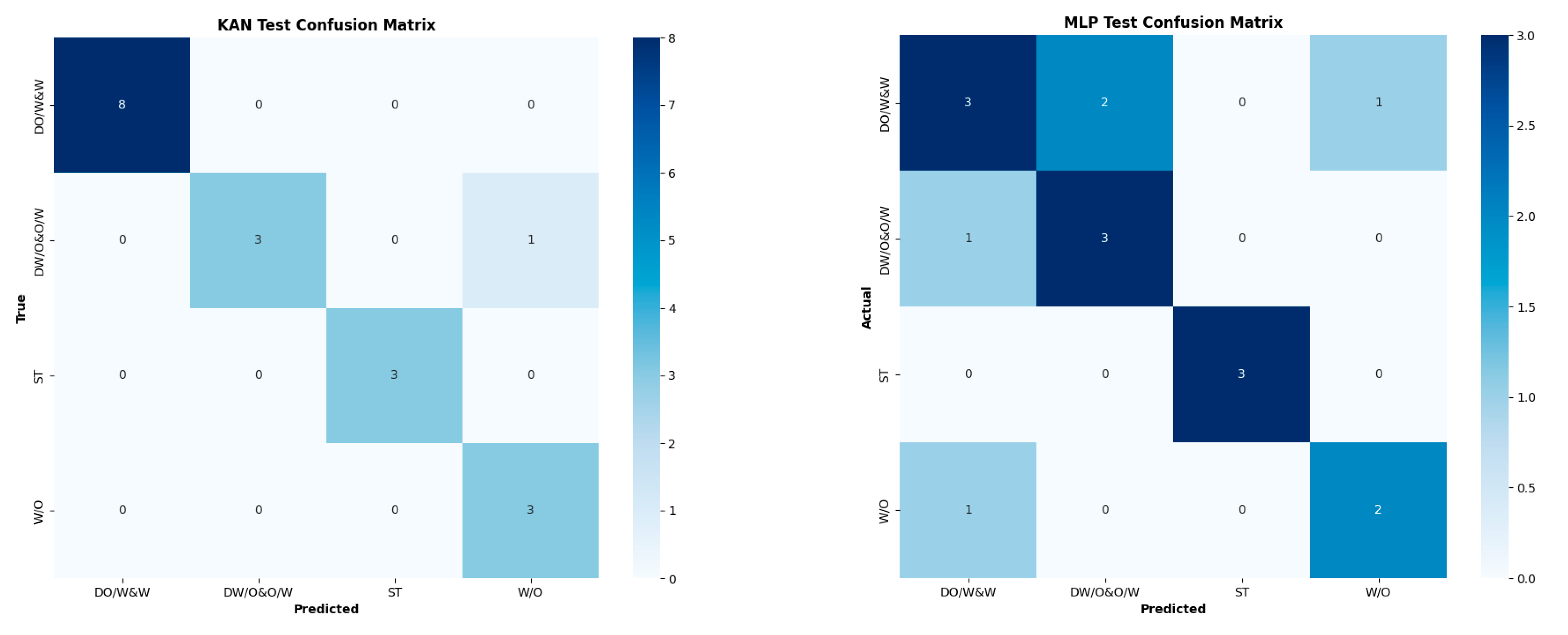
Figure 12 shows the Test Confusion Matrix of KAN and MLP, respectively, which can clearly show whether the prediction effect of the two is good or bad. The horizontal axis represents the flow pattern predicted by the model, while the vertical axis shows the actual flow pattern obtained from the physical experiment. The higher the value on the main diagonal, the more accurate the model’s prediction is. KAN has only one value that is not on the main diagonal, while the image of MLP is rather chaotic, with five values not on the main diagonal.
Table 2 illustrates the prediction results for the MLP neural network across 18 test sample points, whereas Table 3 provides the corresponding results for the KAN model. The bold rows in the table represent the incorrect predictions. By analyzing these two tables, it can be quickly concluded that the MLP neural network prediction error is significant. In contrast, the error of the KAN model prediction is minor.
The MLP neural network exhibits some prediction errors under specific conditions. For instance, when the well inclination is 0 degrees (vertical up), the flow rate is moderate, and the water cut is low, DO/W&W is incorrectly predicted as DO/W&O/W. Similarly, when the well slope is 60 degrees (upslope), the flow rate is low, and the water cut is low, DO/W&W is predicted as O/W. When the well slope is 85 degrees (updip), the flow rate is high, and the water cut is moderate, W/O is predicted as DO/W&W. Additionally, when the well inclination is 90 degrees (horizontal), the flow rate is moderate, and the water cut is low, DO/W&O/W is predicted as DO/W&W. In contrast, the KAN model demonstrates smaller prediction errors than the MLP neural network. For example, when the well slope is 60 degrees (upslope), the flow rate is moderate, and the water cut is high, DW/O&O/W is accurately predicted as W/O. Overall, the KAN model’s predictions align well with the experimental results, whereas the MLP neural network’s predictions show larger discrepancies.
In addition, in this study, both KAN and MLP were provided with two hidden layers, but only seven neurons were provided in each hidden layer of KAN. In contrast, 12 neurons were required in the first hidden layer of MLP and six neurons in the second hidden layer. The accuracy of the prediction results combined with the actual training of KAN and MLP shows that KAN is superior to MLP in predicting patterns of two-phase flow involving oil and water.

6. Conclusions

This paper primarily investigates the utilization of KAN for forecasting patterns of two-phase flow involving oil and water. It compares their performance with the traditional MLP neural network. The research findings demonstrate that KAN achieves greater accuracy in predicting the flow configurations of oil–water mixtures. Experimental validation indicates that the KAN model’s predictions under various operating conditions closely match the flow configurations. KAN exhibits higher training efficiency, with a significantly lower training loss value than the MLP network. As a result, KAN can monitor production logging records in real time. Implementing this approach to forecast additional uncertain factors in oil fields, like solid deposits, can safeguard the reliable functioning of production facilities, markedly lower operational expenses, and fulfill stringent production efficiency demands, thus possessing substantial practical significance in engineering applications.
Recognizing the significant differences between the surface experimental environment and the downhole logging environment is essential. Directly using the experimental results can cause mistakes. When using the KAN model to interpret multiphase flow in production logging downhole, we still need to check if its calculations are accurate.

Author Contributions

Conceptualization, M.O. and H.G.; methodology, M.O.; software, M.O.; validation, L.Y., W.P. and Y.S.; formal analysis, Y.G.; investigation, A.L.; resources, Y.S.; data curation, D.W.; writing—original draft preparation, M.O.; writing—review and editing, L.Y.; visualization, M.O.; supervision, H.G.; project administration, H.G.; funding acquisition, H.G. All authors have read and agreed to the published version of the manuscript.

Funding

This research received no external funding.

Data Availability Statement

The data that support the findings of this study are available from Yangtze University but restrictions apply to the availability of these data, which were used under license for the current study, and so are not publicly available. Data are however available from the authors upon reasonable request and with permission of Yangtze University.

Conflicts of Interest

The authors declare no conflicts of interest.

Abbreviations

The following abbreviations are used in this manuscript:
KANKolmogorov–Arnold Networks
MLPMulti-Layer Perceptron
SSSmooth Stratified Flow
W/OWater in Oil Emulsion
ST & MIStratified Flow with Mixing at the Interface
DO/WDispersion of Oil in Water and Water
DW/O&O/WDispersions of Water in Oil and Oil in Water

References

  1. Puneett, B.; Anupama, R.; Richa, M. Understanding critical service factors in neobanks: Crafting strategies through text mining. J. Model. Manag. 2025, 20, 894–922. [Google Scholar]
  2. Amrita, C. Financial inclusion, information and communication technology diffusion, and economic growth: A panel data analysis. Inf. Technol. Dev. 2020, 26, 607–635. [Google Scholar] [CrossRef]
  3. Wei, J.; Xin, W.; Shu, Z. Integrating multi-modal data into AFSA-LSTM model for real-time oil production prediction. Energy 2023, 279, 127935. [Google Scholar]
  4. Shammre, A.S.A.; Chidmi, B. Oil Price Forecasting Using FRED Data: A Comparison between Some Alternative Models. Energies 2023, 16, 4451. [Google Scholar] [CrossRef]
  5. Al-Tarawneh, M.A.; Al-irr, O.; Al-Maaitah, K.S.; Kanj, H.; Aly, W.H.F. Enhancing Fake News Detection with Word Embedding: A Machine Learning and Deep Learning Approach. Computers 2024, 13, 239. [Google Scholar] [CrossRef]
  6. Chaudhuri, R.; Chatterjee, S.; Vrontis, D.; Thrassou, A. Adoption of robust business analytics for product innovation and organizational performance: The mediating role of organizational data-driven culture. Ann. Oper. Res. 2021, 339, 1–35. [Google Scholar] [CrossRef]
  7. Bassam, A.M.; Phillips, A.B.; Turnock, S.R.; Wilson, P.A. Artificial neural network based prediction of ship speed under operating conditions for operational optimization. Ocean Eng. 2023, 278, 114613. [Google Scholar] [CrossRef]
  8. Vahid, A.; Ataallah, S.; Saeid, S. Robust prediction and optimization of gasoline quality using data-driven adaptive modeling for a light naphtha isomerization reactor. Fuel 2022, 328, 125304. [Google Scholar] [CrossRef]
  9. Yang, C.; Chen, Y.; Li, Y.; Chen, P. A data-driven approach for oil production prediction and water injection recommendation in well groups. Geoenergy Sci. Eng. 2025, 247, 213682. [Google Scholar] [CrossRef]
  10. Xie, J.; Jia, C.; Wang, Z. Data-driven machine-learning models for predicting non-uniform confinement effects of FRP-confined concrete. Structures 2025, 74, 108555. [Google Scholar] [CrossRef]
  11. Talpur, S.A.; Thansirichaisree, P.; Anotaipaiboon, W.; Mohamad, H.; Zhou, M.; Ejaz, A.; Hussain, Q.; Saingam, P.; Chaimahawan, P. Data-driven prediction of failure loads in low-cost FRP-confined reinforced concrete beams. Compos. Part C Open Access 2025, 17, 100579. [Google Scholar] [CrossRef]
  12. Qi, W.L.; Wang, R.; Yang, M.S.; Pan, Z.R.; Liu, K.Z. Data-driven dynamic periodic event-triggered control for unknown linear systems: A hybrid system approach. Syst. Control Lett. 2025, 199, 106067. [Google Scholar] [CrossRef]
  13. Li, X.; Liu, Y.; Zhang, R.; Zhang, N. Probabilistic failure assessment of oil and gas gathering pipelines using machine learning approach. Reliab. Eng. Syst. Saf. 2025, 256, 110747. [Google Scholar] [CrossRef]
  14. Komara, E.; Nugraha, M.F.; Rafi, M.; Lestari, W. Lithology Prediction Using K-Nearest Neighbors (KNN) Algorithm Study Case in Upper Cibulakan Formation. IOP Conf. Ser. Earth Environ. Sci. 2024, 1418, 012062. [Google Scholar] [CrossRef]
  15. Madamanchi, A.; Rabbi, F.; Sokolov, A.M.; Hossain, N.U.I. A Machine Learning-Based Corrosion Level Prediction in the Oil and Gas Industry. Eng. Proc. 2024, 76, 38. [Google Scholar]
  16. Wang, H.; Guo, Z.; Kong, X.; Zhang, X.; Wang, P.; Shan, Y. Application of Machine Learning for Shale Oil and Gas “Sweet Spots” Prediction. Energies 2024, 17, 2191. [Google Scholar] [CrossRef]
  17. Ashraf, M.W.; Dua, V. Data Information integrated Neural Network (DINN) algorithm for modelling and interpretation performance analysis for energy systems. Energy AI 2024, 16, 100363. [Google Scholar] [CrossRef]
  18. Li, F.; Zurada, J.M.; Liu, Y.; Wu, W. Input Layer Regularization of Multilayer Feedforward Neural Networks. IEEE Access 2017, 5, 10979–10985. [Google Scholar] [CrossRef]
  19. Xu, L.; Klasa, S. Recent advances on techniques and theories of feedforward networks with supervised learning. Sci. Artif. Neural Netw. 1992, 1710, 317–328. [Google Scholar]
  20. Ying, X. An Overview of Overfitting and Its Solutions. J. Phys. Conf. Ser. 2019, 1168, 022022. [Google Scholar] [CrossRef]
  21. Liu, Z.; Wang, Y.; Vaidya, S.; Ruehle, F.; Halverson, J.; Soljačić, M.; Hou, T.J.; Tegmark, M. KAN: Kolmogorov-Arnold networks. arXiv 2024, arXiv:2404.19756. [Google Scholar]
  22. Yu, R.; Yu, W.; Wang, X. Kan or mlp: A fairer comparison. arXiv 2024, arXiv:2407.16674. [Google Scholar]
  23. Shukla, K.; Toscano, J.D.; Wang, Z.; Zou, Z.; Karniadakis, G.E. A comprehensive and fair comparison between mlp and kan representations for differential equations and operator networks. Comput. Methods Appl. Mech. Eng. 2024, 431, 117290. [Google Scholar] [CrossRef]
  24. Xu, K.; Chen, L.; Wang, S. Kolmogorov-Arnold networks for time series: Bridging predictive power and interpretability. arXiv 2024, arXiv:2406.02496. [Google Scholar]
  25. Guo, C.; Sun, L.; Li, S.; Yuan, Z.; Wang, C. Physics-informed Kolmogorov-Arnold Network with Chebyshev polynomials for fluid mechanics. arXiv 2024, arXiv:2411.04516. [Google Scholar]
  26. Qiu, B.; Zhang, J.; Yang, Y.; Qin, G.; Zhou, Z.; Ying, C. Research on Oil Well Production Prediction Based on GRU-KAN Model Optimized by PSO. Energies 2024, 17, 5502. [Google Scholar] [CrossRef]
  27. Brill, J.P. Multiphase flow in wells. J. Pet. Technol. 1987, 39, 15–21. [Google Scholar] [CrossRef]
  28. Wu, Y.; Guo, H.; Song, H.; Deng, R. Fuzzy inference system application for oil-water flow patterns identification. Energy 2022, 239, 122359. [Google Scholar] [CrossRef]
  29. Riedmiller, M. Multi Layer Perceptron. Machine Learning Lab Special Lecture; University of Freiburg: Freiburg, Germany, 2014; 139p. [Google Scholar]
  30. Abdurrakhman, A.; Sutiarso, L.; Ainuri, M.; Ushada, M.; Islam, M.P. A Multilayer Perceptron Feedforward Neural Network and Particle Swarm Optimization Algorithm for Optimizing Biogas Production. Energies 2025, 18, 1002. [Google Scholar] [CrossRef]
  31. Tasha, N.; Nima, M. Understanding the Representation and Computation of Multilayer Perceptrons: A Case Study in Speech Recognition. Proc. Mach. Learn. Res. 2017, 70, 2564–2573. [Google Scholar]
  32. Malavika, A.; Pai, L.M.; Johny, K. Ocean subsurface temperature prediction using an improved hybrid model combining ensemble empirical mode decomposition and deep multi-layer perceptron (EEMD-MLP-DL). Remote Sens. Appl. Soc. Environ. 2025, 38, 101556. [Google Scholar] [CrossRef]
  33. Zhang, X.; Cheng, Y.; Chen, H.; Cheng, H.; Gao, Y. Refrigerant charge fault diagnosis in VRF systems using Kolmogorov-Arnold networks and their convolutional variants: A comparative analysis with traditional models. Energy Build. 2025, 336, 15608. [Google Scholar] [CrossRef]
  34. Zhang, L.; Liu, T. ATP-Pred: Prediction of Protein-ATP Binding Residues via Fusion of Residue-Level Embeddings and Kolmogorov-Arnold Network. J. Chem. Inf. Model. 2025, 65, 3812–3826. [Google Scholar] [CrossRef]
  35. Zheng, B.; Chen, Y.; Wang, C.; Heidari, A.A.; Liu, L.; Chen, H.; Liang, G. Kolmogorov-Arnold networks guided whale optimization algorithm for feature selection in medical datasets. J. Big Data 2025, 12, 69. [Google Scholar] [CrossRef]
  36. Nädler, M.; Mewes, D. Flow induced emulsification in the flow of two immiscible liquids in horizontal pipes. Int. J. Multiph. Flow 1997, 23, 55–68. [Google Scholar] [CrossRef]
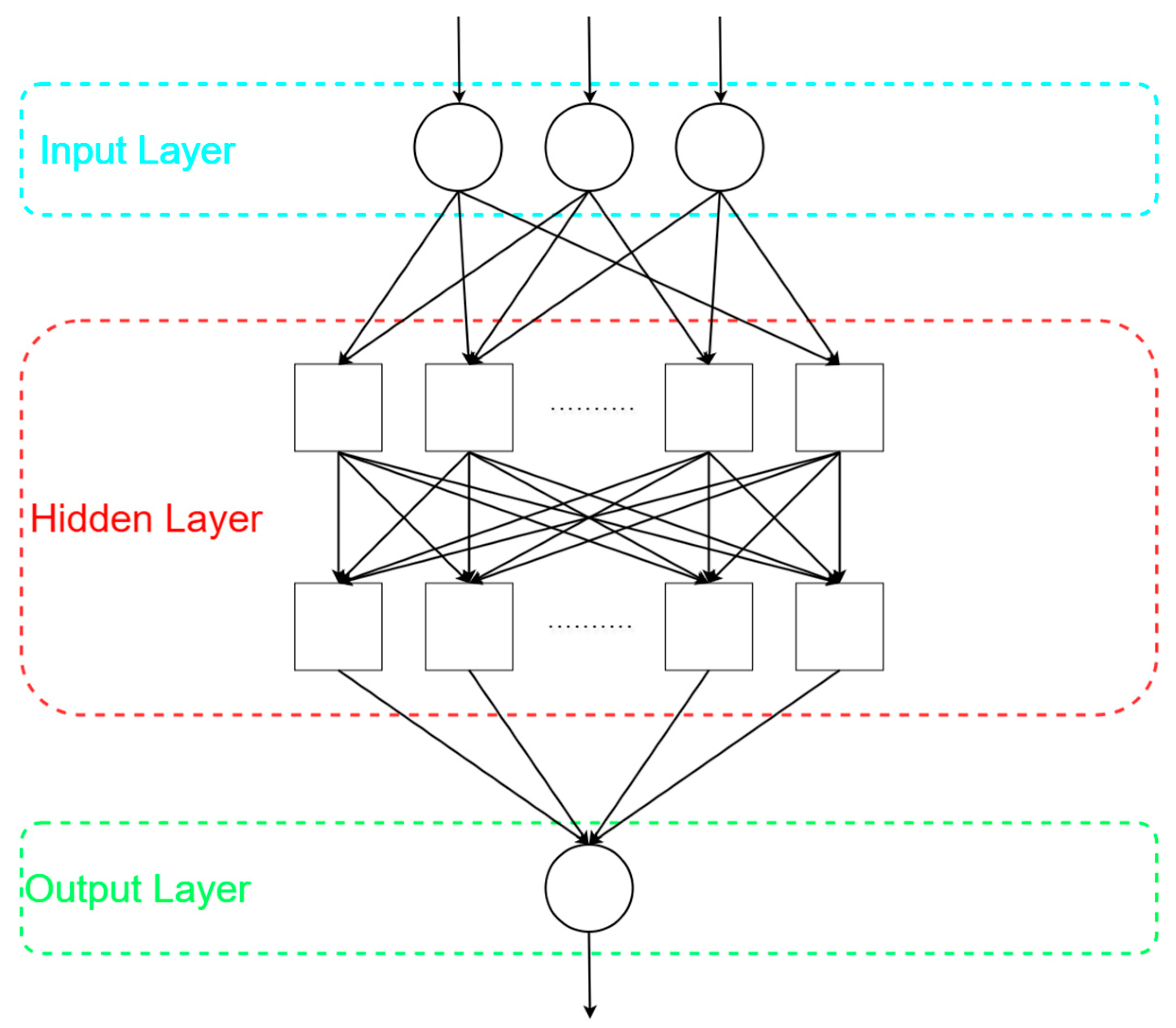
Figure 1. MLP with two hidden layers model diagram.
Processes 13 02562 g001
Figure 2. KAN model diagram.
Processes 13 02562 g002
Figure 3. Schematic of experimental setup. 1—simulation borehole simulator, 2—well deviation regulator, 3—oil–water mixer, 4—positioning control valve, 5—flow meter, 6—pump, 7—water storage tank, 8—oil storage tank, 9—phase separator.
Processes 13 02562 g003
Figure 4. A photograph of the actual RAT device.
Processes 13 02562 g004
Figure 5. A photograph of the actual CAT device.
Processes 13 02562 g005
Figure 6. Comparison of theoretical (left) and experimental (right) flow patterns.
Processes 13 02562 g006
Figure 7. (a) illustrates the flow pattern for vertical upward flow (0°). (b) depicts the flow pattern at an inclination angle of 60°. (c) shows the flow pattern at an inclination angle of 85°. (d) presents the flow pattern for horizontal flow (90°).
Processes 13 02562 g007
Figure 8. MLP neural network training process.
Processes 13 02562 g008
Figure 9. MLP training results.
Processes 13 02562 g009
Figure 10. KAN training process.
Processes 13 02562 g010
Figure 11. KAN training results.
Processes 13 02562 g011
Figure 12. Left is the confusion matrix of the KAN test set. Right is the confusion matrix of the MLP test set.
Processes 13 02562 g012
Table 1. Numerical representation of flow patterns.
Flow PatternNum
W/O0
ST1
DO/W2
DW/O&O/W3
Table 2. Flow pattern prediction results of MLP test points.
Well Angle (°)Flow Rate (m3/Day)Water Cut (%)Oil Density (g/cm3)Water Density (g/cm3)Actual PatternPredicted Pattern
0100800.82630.9884DO/W&WDO/W&W
0100900.82630.9884DO/W&WDO/W&W
0300200.82630.9884DO/W&WDW/O&O/W
0300400.82630.9884DO/W&WDW/O&O/W
0600200.82630.9884W/OW/O
60100200.82630.9884DO/W&WDO/W&W
60100400.82630.9884DO/W&WW/O
60300600.82630.9884W/OW/O
60300800.82630.9884DW/O&O/WDW/O&O/W
60600900.82630.9884DW/O&O/WDW/O&O/W
85100200.82630.9884STST
85100900.82630.9884STST
85300800.82630.9884DO/W&WDO/W&W
85300900.82630.9884DO/W&WDO/W&W
85600600.82630.9884W/ODO/W&W
90100800.82630.9884STST
90300400.82630.9884DW/O&O/WDW/O&W
90600800.82630.9884DW/O&O/WDW/O&O/W
Table 3. Flow pattern prediction results of KAN test points.
Well Angle (°)Flow Rate (m3/Day)Water Cut (%)Oil Density (g/cm3)Water Density (g/cm3)Actual PatternPredicted Pattern
0100800.82630.9884DO/W&WDO/W&W
0100900.82630.9884DO/W&WDO/W&W
0300200.82630.9884DO/W&WDO/W&W
0300400.82630.9884DO/W&WDO/W&W
0600200.82630.9884W/OW/O
60100200.82630.9884DO/W&WDO/W&W
60100400.82630.9884DO/W&WDO/W&W
60300600.82630.9884W/OW/O
60300800.82630.9884DW/O&O/WW/O
60600900.82630.9884DW/O&O/WDW/O&O/W
85100200.82630.9884STST
85100900.82630.9884STST
85300800.82630.9884DO/W&WDO/W&W
85300900.82630.9884DO/W&WDO/W&W
85600600.82630.9884W/OW/O
90100800.82630.9884STST
90300400.82630.9884DW/O&O/WDW/O&O/W
90600800.82630.9884DW/O&O/WDW/O&O/W
Disclaimer/Publisher’s Note: The statements, opinions and data contained in all publications are solely those of the individual author(s) and contributor(s) and not of MDPI and/or the editor(s). MDPI and/or the editor(s) disclaim responsibility for any injury to people or property resulting from any ideas, methods, instructions or products referred to in the content.