Abstract
South Africa’s transition to a renewable-powered grid faces critical challenges due to the inherent variability of wind and solar generation as well as the need for economically viable and reliable dispatch strategies. This study proposes a scenario-based stochastic optimization framework that integrates machine learning forecasting and uncertainty modeling to enhance operational decision making. A hybrid Long Short-Term Memory–XGBoost model is employed to forecast wind, photovoltaic (PV) power, concentrated solar power (CSP), and electricity demand, with Monte Carlo dropout and quantile regression used for uncertainty quantification. Scenarios are generated using appropriate probability distributions and are reduced via Temporal-Aware K-Means Scenario Reduction for tractability. A two-stage stochastic program then optimizes power dispatch under uncertainty, benchmarked against Deterministic, Rule-Based, and Perfect Information models. Simulation results over 7 days using five years of real-world South African energy data show that the stochastic model strikes a favorable balance between cost and reliability. It incurs a total system cost of ZAR 1.748 billion, with 1625 MWh of load shedding and 1283 MWh of curtailment, significantly outperforming the deterministic model (ZAR 1.763 billion; 3538 MWh load shedding; 59 MWh curtailment) and the rule-based model (ZAR 1.760 billion, 1.809 MWh load shedding; 1475 MWh curtailment). The proposed stochastic framework demonstrates strong potential for improving renewable integration, reducing system penalties, and enhancing grid resilience in the face of forecast uncertainty.
1. Introduction
South Africa is endowed with substantial renewable energy (RE) potential, particularly in wind and solar resources [1]. Yet, the country relies heavily on coal-fired power plants, which account for approximately 80% of its electricity generation [2,3]. Renewable energy resources offer a transformative opportunity to enhance the sustainability of the nation’s energy system, reducing reliance on fossil fuels and mitigating environmental impacts [4]. Despite these benefits, the integration of RE sources into the national grid remains limited, primarily due to their intermittent and stochastic nature [5,6]. Wind power varies with weather conditions, and photovoltaic (PV) generation is unavailable at night, which creates significant challenges for grid stability and operational cost management. In isolated power grids, such as those in small island systems, these issues are exacerbated, as mismanaged RE resources, particularly wind turbines, can destabilize the grid, affecting power storage, frequency stabilization, and overall system reliability [7].
Furthermore, the integration of RE sources into power grids introduces challenges related to grid inertia [8], a property inherent in traditional non-renewable generators but often absent in RE systems [9]. Wind turbines, for instance, are typically not directly coupled to the grid and use inverters to manage frequency stability, which limits their ability to provide inertia [10]. Similarly, PV panels, being static devices, cannot generate rotational inertia. Grid inertia is critical in mitigating frequency drops by enabling the system to respond to sudden increases in load demand [10].
Thus, highly accurate models are needed to predict sudden load increases. Figure 1 illustrates a schematic of a centrally controlled national grid that integrates RE sources. The Grid Control Center (GCC) serves as the core authority that dispatches energy and makes real-time operational decisions. It coordinates conventional power plants, renewable sources, energy storage systems, and national electricity demand [11]. The GCC ensures optimal power flow, preserves system reliability, and maintains equilibrium between supply and demand despite fluctuations in generation. In essence, integrating RE into the grid necessitates that operators anticipate sudden demand spikes to prevent frequency deviations and rapidly adjust system operations to maintain grid stability. Addressing these challenges demands advanced optimization strategies capable of handling uncertainty in both renewable generation and electricity consumption. These methods must also optimize storage use, reduce operational costs, and support stable and cost-effective use of renewable resources [12,13].
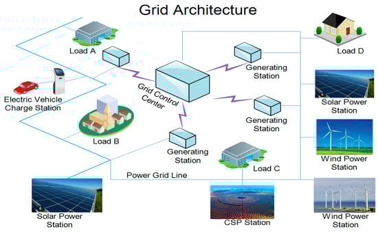
Figure 1.
Schematic representation of a centrally controlled national grid with integrated renewable energy sources.
Ramadan et al. [14] proposed a framework for the optimal planning of distribution systems, incorporating renewable-based distributed generators (DGs) while addressing uncertainties in load and generation. The model employed a multi-objective formulation to minimize expected power loss, voltage deviation, system cost, and emissions, while enhancing overall voltage stability. The Equilibrium Optimizer (EO) algorithm was used to determine optimal DG sizes and locations, with validation performed on IEEE 69-bus and 94-bus practical distribution systems. Although this framework demonstrated notable performance improvements, such as a 70.66% emission reduction and a 48.73% increase in voltage stability on the 69-bus system, it was focused on long-term planning and static optimization. Niknami et al. [15] introduced a two-step optimization model, Robust Day-Ahead Scheduling for Enhanced Resilience, to manage microgrid energy amidst renewable integration, uncertain demand, and diverse equipment like batteries and electric vehicles, achieving an 8% cost reduction over existing methods by optimizing energy use, battery management, and distributed generation dispatch using a Column-and-Constraint Generation (C&CG) algorithm. Additionally, Li et al. [16] proposed a two-stage stochastic optimization framework for multi-energy microgrids using CVaR to address risk from renewable and load uncertainties, with scenario generation via Monte Carlo simulation and improved K-means clustering. While their approach was effective at the microgrid scale, it failed to account for constraints peculiar to a national grid, such as reserve adequacy, the startup/shutdown dynamics of generators, large-scale curtailment management, and system-wide load shedding penalties, all of which are crucial for ensuring grid-wide reliability and operational feasibility.
Mathur et al. [17] developed a priority-based cost optimization framework for hybrid PV–wind-controllable distributed generator microgrids, addressing the intermittent nature of RE sources through a stochastic day-ahead scheduling strategy that minimizes costs using the Grey Wolf Optimization (GWO) algorithm. Their work outperformed the Jaya and Particle Swarm Optimization (PSO) algorithms with optimal costs of USD 3754 (best case) versus USD 4222 for Jaya on the CIGRE test network, though costs increased in isolated mode due to load curtailment. Zhang et al. [18] introduced a stochastic optimization framework for integrated energy microgrid operations using a time-divided scenario generation method based on forecasting errors in PV and load. Their methodology, applied to a microgrid in Changzhou, Jiangsu Province, China, constructed probabilistic models using nonparametric kernel density estimation (KDE) to capture distribution characteristics and time correlation of uncertainties. While Zhang et al.’s method is based on synthetic error modeling, our work applies real empirical energy data from the South African grid to derive more context-specific insights into renewable uncertainty. Other research efforts in renewable uncertainty and their mitigation techniques for grid integration can be found in [19,20,21,22]
Despite growing research in RE integration, current approaches often fall short in three critical areas: (i) many focus on microgrid or small-scale systems and do not address the operational complexities of national grids; (ii) forecasting and dispatch are often treated as separate, decoupled tasks; and (iii) uncertainty quantification is either absent or insufficiently integrated into decision making. As detailed in our literature review, existing models, such as those by Ramadan et al. [14], Niknami et al. [15], Li et al. [16], Mathur et al. [17], and Zhang et al. [18], have demonstrated valuable contributions in distribution system planning, microgrid scheduling, and risk-aware optimization. However, most of these works rely on synthetic data, focus on isolated systems, or neglect key reliability metrics like curtailment and load shedding under uncertainty.
To address these gaps, this study proposes a unified, scenario-based stochastic optimization framework that integrates machine learning-based forecasting, probabilistic scenario generation, and dispatch optimization under uncertainty. We apply the proposed framework to five years of real-world data from the South African power grid to benchmark four dispatch strategies—stochastic, deterministic, rule-based, and perfect information. The objective is to demonstrate the practical benefits of our approach in enhancing cost efficiency, system resilience, and RE integration in high-variability power systems. In essence, the primary contributions of this work are threefold:
- Hybrid forecasting with uncertainty quantification: We develop an LSTM–XGBoost hybrid model for forecasting wind, PV power, concentrated solar power (CSP) generation, and electricity demand that integrates Monte Carlo dropout and quantile regression to capture predictive uncertainty. This is crucial for informed scenario generation in stochastic planning.
- Physically and statistically grounded scenario generation and reduction: We introduce a distribution-based sampling framework using Weibull (wind), Beta (solar), and Lognormal (demand) distributions combined with turbine power curves and diurnal constraints to generate realistic input scenarios and reduced via a Temporal-Aware K-Means Scenario Reduction process for computational efficiency.
- Stochastic optimization and real data evaluation: A two-stage stochastic optimization framework is developed and evaluated using five years of national grid data from South Africa.
2. Problem Description and Data Overview
2.1. Problem Formulation
The short-term scheduling problem under RE uncertainty is formulated as a scenario-based stochastic mixed-integer linear programming (MILP) model. MILP was chosen for its ability to handle both binary and continuous decision variables while efficiently optimizing across multiple scenarios, which makes it well suited for capturing uncertainty in renewable generation and system constraints within a stochastic framework. The system’s objective is to minimize the total expected system cost while ensuring operational feasibility across all considered scenarios. Table 1, Table 2 and Table 3 define the sets and indexes, decision variables, and parameters employed in the formulation of the MILP model.

Table 1.
Sets and indexes of the MILP model.
Table 2.
Decision variables of the MILP model.
Table 3.
Parameters of the MILP model.
2.2. Objective Function
The objective function is to minimize the expected total cost:
System Constraints
The dispatch optimization problem is subject to a set of operational and reliability constraints to ensure feasible and realistic power system operation under uncertainty. While this model abstracts from detailed network constraints such as AC power flow equations, it provides a high-level, system-wide dispatch optimization approach focused on uncertainty and generation-side planning. The key constraints are defined as follows.
- i.
- Power Balance
At each time t, and for each scenario :
- ii.
- Generator Operating Limits
- iii.
- Storage Dynamics
- iv.
- Startup/Shutdown
Binary variables for generator on/off status () define startup and shutdown events:
- v.
- Minimum Up/Down Time
To ensure operational consistency, each generator must satisfy minimum uptime and downtime requirements as follows:
- vi.
- Non-Negativity
Load shedding and curtailment values cannot be negative:
- vii.
- Spinning Reserve Requirement
Enough total reserve must be available at each time step:
- viii.
- Reserve Limits
Reserve must be within each generator’s available headroom:
- ix.
- Coal Emission Limit Constraint
To model the environmental compliance of coal-fired generators, we use
- x.
- Coal Fuel Availability Constraint
To reflect finite coal stock, we use
- xi.
- Partial-Load Efficiency Penalty
To account for efficiency degradation at low outputs, we use
2.3. Data Overview
2.3.1. Dataset Description
This study utilizes two complementary datasets obtained from Eskom [23] and the Climate Information Portal [24], spanning five years (January 2020 to December 2024), in order to develop and validate the proposed framework for dispatch optimization and RE utilization. The first is an energy dataset capturing hourly RE generation, installed capacities, non-RE supply, and total demand. The second is a weather dataset providing hourly meteorological conditions, which are critical for RE forecasting.
2.3.2. Energy Dataset
The dataset includes 42,623 hourly energy records from 1 April 2020, to 9 February 2025, for South Africa’s power system obtained from Eskom [23]. It covers generation data for wind, solar PV, CSP, and other renewable sources, along with total electricity demand and supply. Among renewable sources, wind energy is the largest contributor, with an average generation of ~1103 MW and a maximum of ~3102 MW, supported by installed capacities ranging from 2080 MW to 3443 MW. Solar PV has a maximum generation of 2155 MW and an average of 565.8 MW. CSP reaches a maximum of 499 MW and averages 168.57 MW. The total RE generation averages around 1860 MW, peaking above 5100 MW. In terms of installed capacity, wind is valued at 3442.99 MW, PV at 2287.43 MW, CSP at 500 MW and other renewables at 50.88 MW. Figure 2 presents the monthly time series of energy generation in South Africa from April 2020 to February 2025.
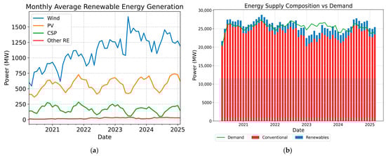
Figure 2.
(a). Monthly time series of energy generation in South Africa from April 2020 to February 2025 (b). (b) illustrates trends and variability across different renewable and non-RE sources. It also reveals a supply and demand gap from 2023 to 2024.
2.3.3. Weather Dataset
The weather dataset, sourced from the Climate Information Portal [24], includes five years of hourly data covering key environmental variables such as wind speed, temperature, humidity, rainfall, solar radiation, and sunshine hours. To align with the national energy dataset, weather data were collected from provinces with dominant RE infrastructure; wind-related data came from the Eastern and Western Cape, and solar-related data came from the Northern Cape. The data was spatially aggregated using hourly averages to approximate nationwide conditions. This aggregated dataset was synchronized with national energy records for forecasting model training. Key patterns included average wind speeds of 2.96 m/s with peaks up to 35.68 m/s, temperatures ranging from −4.14 °C to 41.9 °C, and highly variable humidity. Rainfall and solar radiation showed skewed distributions, while sunshine hours, wind direction, and evapotranspiration provided further insights into the variability influencing renewable generation.
2.3.4. Data Integration and Preprocessing
To ensure data readiness for forecasting and optimization tasks, both weather and energy datasets were subjected to systematic preprocessing and alignment. Energy records were timestamped using the ‘Date Time Hour Beginning’ field, while weather records required conversion from a non-standard 24:00 format, which was normalized to 00:00 of the following day. All time stamps were converted to date–time objects to ensure temporal synchronization across datasets. Datasets were then merged by intersecting their valid time ranges, preserving only the overlapping periods to ensure aligned observations between weather features (e.g., wind speed) and energy outputs (e.g., wind and solar generation). Missing values were imputed using forward and backward fill techniques, a common method in time series preprocessing used to maintain data continuity without introducing artificial noise [25]. Unit consistency was enforced (e.g., MW for generation and m/s for wind speed) to preserve the physical interpretability of the data [26].
To validate the alignment and internal consistency of features, visual inspections were performed. For example, we plotted wind speed against wind energy output to confirm expected correlations. These preprocessing steps are crucial for building machine learning models, particularly Long Short-Term Memory (LSTM) networks, which require input features to be scaled and reshaped into fixed-length temporal sequences. Min–max scaling was applied to both features and targets to standardize input ranges and improve convergence behavior during training [27]. Figure 3 presents an overview of the data preprocessing and integration workflow.
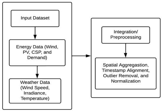
Figure 3.
Overview of the data preprocessing and integration workflow.
3. Methodology
This research employs a scenario-based stochastic optimization framework that integrates machine learning-based forecasting with uncertainty modeling to enhance power dispatch planning. As illustrated in Figure 4, the method comprises two main phases: (1) A hybrid LSTM–XGBoost model generates forecasts and prediction intervals for PV, wind, CSP, and demand, with uncertainty quantified through Monte Carlo dropout and quantile regression. These probabilistic forecasts are used to produce multiple scenarios, which are reduced using Temporal-Aware K-Means clustering to ensure computational efficiency. (2) A two-stage stochastic MILP model is then used for dispatch optimization, where the first stage determines day-ahead unit commitment and storage operations, and the second stage optimizes real-time dispatch across all scenarios. This end-to-end framework is designed to enable robust and cost-effective decision making under renewable generation uncertainty. Figure 4 presents an overview of the proposed framework.
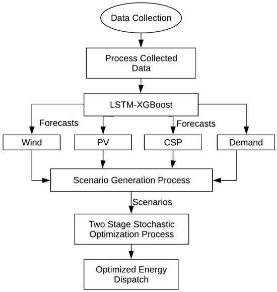
Figure 4.
Proposed data-driven stochastic optimization framework.
3.1. Hybrid LSTM–XGBoost Model
The forecasting component of the framework utilizes a hybrid model that combines Long Short-Term Memory (LSTM) networks with Extreme Gradient Boosting (XGBoost) to predict energy generation from wind, PV, and CSP, as well as total energy demand. LSTM, a form of recurrent neural network, is well suited for capturing temporal dependencies and sequential patterns [28,29,30], making it ideal for modeling the daily and seasonal fluctuations inherent in RE data [31]. Its ability to retain long-range dependencies enables accurate forecasting of time series behavior over extended horizons [32,33]. To improve the model’s overall robustness and accuracy, XGBoost is integrated to capture complex non-linear relationships and interactions across multiple features. The hybrid approach is deliberately designed to leverage LSTM’s sequential learning capabilities alongside XGBoost’s gradient-boosting efficiency in order to ensure more reliable and precise forecasts [34]. This dual-model strategy plays a critical role in the downstream optimization process, with improved energy scheduling and greater grid resilience under RE variability.
In this architecture, the Long Short-Term Memory (LSTM) network is tasked with modeling the sequential behavior of RE generation (wind, PV, and CSP), relevant weather parameters (e.g., time, wind speed, temperature, and solar radiation), and electricity demand. These input variables exhibit diurnal and seasonal patterns that the LSTM captures through its recurrent connections and memory cell, enabling it to learn long-term dependencies. For example, the model learns how patterns in wind speed affect wind energy production over time or how solar radiation impacts PV output throughout the day.
The LSTM’s learned representations, which encapsulate both short-term fluctuations and long-range dependencies, are then passed as input features to the XGBoost model. XGBoost further refines the predictions by modeling complex, non-linear interactions that may not be fully captured by the LSTM alone, thereby enhancing overall forecasting accuracy. LSTM’s internal operations are governed by a set of gating mechanisms that regulate the flow of information through time. Specifically, the memory cell is updated using Equations (18)–(22) [35].
where , , and are the forget, input, and output gates; is the memory cell; and is the hidden state.
XGBoost, a gradient-boosting framework, refines the LSTM predictions by incorporating additional features and capturing non-linear interactions that the LSTM might miss. For instance, XGBoost can model the interaction between wind degree and temperature to improve WIND predictions or use radiation and humidity to enhance PV forecasts. The hybrid model is trained on historical data, with the LSTM handling the temporal dynamics and XGBoost optimizing the final predictions. To provide probabilistic forecasts, Monte Carlo dropout is applied in the LSTM layer to generate a distribution of predictions, and XGBoost’s quantile regression capabilities are used to estimate uncertainty bounds (e.g., 10th, 50th, and 90th percentiles). This results in a range of scenarios for RE generation and demand, such as high, medium, and low WIND output, which are critical for the stochastic optimization stage. XGBoost minimizes the objective defined in (7) as follows [36]:
where = is the squared error, and = is a regularization term used to avoid overfitting.
The combined prediction is defined as
3.2. Scenario Generation Process
To effectively address the uncertainties associated with RE generation and demand forecasting, we formulate a scenario generation process (SGP) that creates a diverse set of future trajectories for wind, PV, CSP, and total demand over a predefined forecast horizon. The SGP is controlled by four primary inputs: N, the number of scenarios per target; S, the start date of the forecast window; L, the length of the forecast window; and F, a scaling factor to control uncertainty spread. These inputs define the temporal and probabilistic structure of the scenarios used within the optimization framework.
The SGP begins with a Long Short-Term Memory (LSTM) network, which is trained on historical energy and weather datasets to capture underlying temporal dependencies. Given an input sequence , where l denotes the lookback window and d the number of features, the LSTM generates multiple Monte Carlo samples through stochastic forward passes. These samples are used to compute both the mean prediction and the standard deviation which quantifies forecast uncertainty [37].
To increase variability, the standard deviation is scaled by a factor s, i.e.,
Next, the mean prediction is concatenated with relevant exogenous features to form the input vector for an XGBoost model:
To improve the realism of scenario generation for the optimization process, we model uncertainties in wind, solar (PV and CSP), and total demand using distributions that reflect their physical and statistical characteristics. Wind power is modeled using the Weibull distribution, solar generation via the Beta distribution with diurnal constraints, and total demand using the Lognormal distribution to capture positive skewness.
3.2.1. Wind Scenario Sampling (Weibull Distribution)
Wind speeds are sampled from a Weibull distribution characterized by the shape parameter k and scale parameter λ [38] derived from the mean μ and standard deviation σ:
Wind speeds are then converted into power output P(v) using a turbine power curve characterized by cut-in, rated, and cut-out wind speeds.
where , , and , which reflects the total installed wind capacity in the South African grid as of 2024. This value is used to scale the normalized wind power outputs simulated using the Weibull distribution, ensuring physical realism in the generation scenarios.
3.2.2. PV and CSP Scenario Sampling (Beta Distribution)
Solar power (PV and CSP) scenarios are modeled using the Beta distribution [39] after normalizing by the respective maximum capacities (PV: 2287 MW, CSP: 500 MW).
These values represent the maximum recorded or registered generation capacities of grid-connected systems in South Africa during the study period and are critical for scaling stochastic forecasts to realistic operational levels. The Beta distribution is parameterized using the empirical mean μ and standard deviation σ derived from the historical generation data.
Given the mean μ and standard deviation σ [40],
The variance is , and the parameters are estimated as follows [40]:
Samples are then scaled back:
Nighttime hours (20:00–04:00) are set to zero to reflect solar unavailability, i.e.,
3.2.3. Total Demand Scenario Sampling (Lognormal Distribution)
Total demand uncertainty is modeled using the Lognormal distribution to account for positive skewness. The Lognormal distribution is parameterized by and [41]. Given mean μ and standard deviation , both 0.1,
Scenarios are generated and then clipped to realistic system demand limits.
3.3. Temporal-Aware K-Means Scenario Reduction
While generating a large number of scenarios enhances robustness, it significantly increases the computational burden of stochastic optimization [42]. To address this, we propose a Temporal-Aware K-Means Scenario Reduction (TAKSR) method that balances representativeness with computational efficiency while enforcing physical constraints. TAKSR reduces the original scenario set by clustering based on extracted statistical and temporal features and selecting representative scenarios from each cluster.
3.3.1. Feature Extraction
For each scenario i, TAKSR extracts a 28-dimensional feature vector capturing key statistical and temporal characteristics:
where is the time series of scenario i, is the corresponding forecast, is the mean during 06:00–18:00 minus the mean during 18:00–06:00, and the mean deviation is the average deviation from the forecast mean.
The features are then standardized using z-score normalization [43] to ensure comparability across dimensions:
3.3.2. Clustering and Scenario Selection
The standardized feature vectors are clustered using K-Means with K clusters. The optimal number of clusters is selected by maximizing the silhouette score [44]:
where is the intra-cluster distance for point i, and is the nearest-cluster distance. Once clustering is completed, the representative scenario for each cluster k is selected as the closest to the cluster centroid [45]:
The full forecast, scenario selection, and reduction process are summarized in Algorithm 1.
| Algorithm 1: Hybrid Forecasting and Scenario Reduction Process |
| Input: X → Historical multivariate time series data, → Exogenous features at time t, l → Lookback window, k → Number of scenarios, n → Number of LSTM stochastic passes, α → Confidence level (e.g., 90%), S → Start date of forecast window, L → Length of forecast horizon, F → Uncertainty scaling factor |
| Outputs: , , , : Prediction Interval |
|
3.3.3. Temporal and Physical Constraints
To ensure physical realism, especially for solar resources like PV and CSP, TAKSR re-applies temporal constraints after representative scenario selection. Although such constraints are already imposed during scenario generation, reapplying them serves as a safeguard. Specifically, clustering may occasionally select scenarios where noise or forecast deviations push nighttime values slightly above zero. Re-imposing these constraints ensures such anomalies are corrected. Additional constraints include ramping limits during dawn and dusk to reflect realistic solar behavior and clipping to predefined capacity limits for feasibility. Figure 5 presents the workflow from the forecasting model to the scenario generation process.
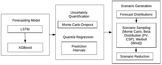
Figure 5.
Forecasting model and the scenario generation workflow.
3.4. Stochastic Optimization Model
We employ a two-stage stochastic programming framework to optimize energy scheduling in both day-ahead and real-time operations. This model incorporates probabilistic scenarios derived from hybrid LSTM–XGBoost forecasts to represent uncertainty in RE generation and electricity demand.
3.4.1. First Stage (Day-Ahead Scheduling)
In the first stage, the model determines the optimal unit commitment of non-RE resources and the preliminary dispatch of renewable resources based on forecasted scenarios. The objective is to minimize the expected cost, which comprises fuel costs for non-renewable generation, startup and shutdown costs, and penalties for potential demand shortfalls. Constraints ensure that the total supply meets forecasted total demand while respecting system capacities (e.g., wind install and PV install). The key decision variables include the binary unit commitment status , startup indicators , and shutdown indicators . The first stage cost is calculated as
3.4.2. Second Stage (Real-Time Scheduling and Recourse Decisions)
The second stage of the two-stage stochastic optimization model addresses real-time operational adjustments in response to forecast deviations in RE generation and load demand. For each scenario, , the model activates scenario-dependent variables that include non-renewable generation levels , , , . These variables allow the model to implement corrective actions that maintain grid balance under uncertainty. For instance, if wind generation underperforms due to low wind speed, the model compensates by increasing non-renewable generation or invoking demand-side adjustments such as load shedding:
The model is formulated as a mixed-integer linear program (MILP) and implemented in Python using Gurobi [46], a high-performance solver capable of handling the combinatorial complexity of large-scale scheduling problems. The optimization spans a 7-day horizon and incorporates operational constraints such as generator capacity limits, minimum up/down times, ramping limits, and storage dynamics. This architecture ensures that anticipatory (first-stage) decisions are made with awareness of potential real-time (second-stage) adjustments, enabling a cost-effective and resilient energy dispatch strategy under RE uncertainty.
3.4.3. Performance Metrics and System Parameters
The model’s performance under forecast uncertainty is evaluated using system-level indicators, as summarized in Table 4. Table 5 outlines the operational parameters used for dispatch simulations. These parameter values are drawn from publicly available sources, including planning documents from Eskom [47] and reports by the Department of Mineral Resources and Energy (DMRE) [48]. Where precise values were not available, reasonable estimates were adopted based on similar studies. All parameters are configurable and can be adjusted to reflect the operational preferences or constraints of specific system operators.
Table 4.
Performance metrics for evaluating the model’s effectiveness.
Table 5.
System parameters.
3.5. Technical Implementation and Computational Setup
The framework was implemented using Python v3.10, with TensorFlow v2.19 and Scikit-learn libraries v1.6 supporting the hybrid LSTM–XGBoost model’s development. The optimization component was developed using Pyomo v6.9 and solved with Gurobi 12.0. The training and simulations were executed on a workstation equipped with an Intel Core i7 processor, 16 GB RAM, and an NVIDIA RTX 3090 GPU. Training the hybrid forecasting model took approximately 3.2 h across all four targets. The stochastic optimization solver runtime for a full 7-day dispatch problem (across 50 scenarios) averaged 18–22 min per instance.
4. Results and Discussion
The proposed optimization model’s performance is compared with three scheduling models (Deterministic, Rule-Based, and Perfect Information) over a 168 h (7-day) horizon. The Deterministic model assumes a single point forecast and solves all decisions in a single stage without accounting for uncertainty. The Rule-Based model uses fixed threshold-based decisions. The Perfect Information model assumes full knowledge of future energy generation and demand. While not feasible in practice, it provides a theoretical lower bound on operational cost, serving as a performance benchmark. The features of these models, compared in Table 6, provide a basis for analyzing the trade-offs between cost, reliability, and operational flexibility in power systems with high RE integration.
Table 6.
Features of compared optimization models.
4.1. Forecasting Model Performance
The predictive performance of the hybrid LSTM–XGBoost model for each of the target variables was assessed using five standard evaluation metrics: mean absolute error (MAE), root mean square error (RMSE), symmetric mean absolute percentage error (sMAPE), prediction interval coverage probability (PICP), and mean prediction interval width (MPIW). Table 7 summarizes the performance metrics for each target variable. Figure 6 displays time series plots of forecast errors over a 7-day period (2–9 February 2025), while Figure 7 illustrates the predicted versus actual values for all target variables over the same period.
Table 7.
Results of performance metrics for each target.
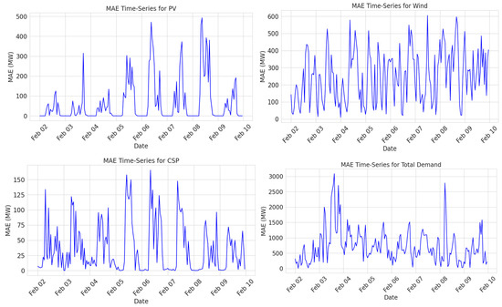
Figure 6.
Time series plots of forecast errors over a 7-day horizon (2–9 February 2025).
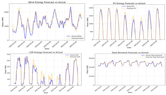
Figure 7.
Predicted vs. actual values for all target variables.
4.1.1. Point Forecast Accuracy (MAE and RMSE)
Wind forecasts recorded the highest absolute errors, with average MAE and RMSE values of 248.15 MW and 289.60 MW, respectively. This reflects the inherent variability and intermittency of wind power, which remains challenging to model due to its stochastic nature. PV and CSP forecasts demonstrated significantly better performance, with lower MAE values (63.97 MW for PV and 35.63 MW for CSP) and RMSE values of 124.46 MW and 53.87 MW, respectively. Notably, demand forecasts resulted in the highest absolute errors (MAE: 729.41 MW, RMSE: 918.35 MW). However, this is expected due to the larger scale of demand values compared to individual renewable generation sources. Despite the large magnitude, the low sMAPE (2.94%) indicates a high degree of relative accuracy, confirming that the model effectively captures demand patterns over time.
The MAE time series plots in Figure 6 highlight distinct error patterns over the test period starting 2 February 2025. Wind forecasts show fluctuating MAE values with regular spikes ranging from 100 to 300 MW, reflecting variable wind conditions. PV and CSP display elevated MAEs during midday peaks, with values between 100 and 500 MW during periods of intense solar activity. Total demand records the highest MAE, reaching up to 3000 MW during the midday peak on 3 February, indicating significant variability in load behavior.
4.1.2. Percentage Error (sMAPE)
The sMAPE values for CSP and PV forecasts were 56.28% and 42.20%, respectively, which may suggest moderate proportional accuracy at first glance. However, these values are largely influenced by frequent periods of low or near-zero generation, such as nighttime (for PV) and cloudy conditions (for CSP), where even small absolute errors can inflate percentage-based metrics. This is a well-known limitation of sMAPE when applied to intermittent renewable sources. In contrast, wind forecasting yielded a lower sMAPE of 18.89%, consistent with its more stable generation profile. Demand forecasting achieved an sMAPE of just 2.94%, which indicates high proportional accuracy and reinforces the model’s effectiveness in load prediction. While sMAPE provides useful insights, it should be interpreted alongside absolute error metrics such as MAE and RMSE, which offer a more practical measure of forecasting performance, particularly for sources with variable output.
4.1.3. Uncertainty Quantification (PICP and MPIW)
The uncertainty quantification results, measured using prediction interval coverage probability (PICP) and mean prediction interval width (MPIW), varied notably across forecast targets. PV forecasts achieved the best balance, with a PICP of 66.15% and an MPIW of 80.23 MW, suggesting reasonably well-calibrated intervals that captured most of the variability without being overly wide. Demand forecasts had a higher MPIW of 319.02 MW, reflecting a more conservative (i.e., wider) interval, yet only a modest PICP of 40.42%, which indicates moderate reliability but excessive uncertainty spread. Wind forecasts, with an MPIW of 98.26 MW and PICP of 39.90%, showed wide intervals that still failed to provide adequate coverage, signaling underfitting of extreme variability. CSP forecasts exhibited the narrowest MPIW (19.52 MW) but the lowest PICP (36.98%), pointing to overconfident intervals that often missed the actual values. In general, the forecasting model captured uncertainty better in PV and demand compared to wind and CSP, but further improvements in interval calibration are needed, especially for solar-based sources.
4.2. Scenario Generation Results
Figure 8 presents the clustered scenarios and the mean forecast between the 2nd and 9th of February 2025. Each figure displays the range of possible outcomes and central tendencies. For total demand, the scenario clusters exhibit a well-defined diurnal cycle, with peak consumption reaching approximately 27,500–30,000 MW and nighttime lows of around 17,500–20,000 MW. The tight grouping around the mean forecast reflects a low degree of forecast uncertainty, attributable to the regularity and predictability of aggregated demand patterns over short time frames.
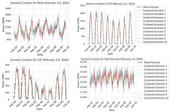
Figure 8.
Scenario cluster and mean forecast between the 2nd and 9th of February 2025.
In contrast, the renewable generation forecasts reveal varying degrees of uncertainty. PV and CSP forecasts display characteristic solar-driven profiles, with daytime peaks of around 2000 MW for PV and 400 MW for CSP. Scenario divergence is most evident during midday peaks, particularly between the 5th and 6th. It reflects the source’s sensitivity to weather variability. These results align with the moderate sMAPE values previously reported for PV and CSP, which emphasize challenges in modeling solar output. Wind forecasts present the greatest variability, with scenarios spanning 500 to 2500 MW and lacking a discernible daily pattern. In some instances, the intrinsic stochasticity of wind resources causes a significant deviation from the mean by over 1000 MW.
4.3. Cost Analysis
Figure 9 presents the total operational costs of the four energy dispatch models. The cost comprises non-renewable generation cost, storage cost, penalty costs for load shedding, and curtailment. As expected, the Perfect Information model, which served as the theoretical benchmark, achieved the lowest total cost (ZAR 1.690 billion) by assuming complete foresight of future demand and renewable generation. In contrast, the Deterministic model, which assumes a single point forecast and solves all decisions in a single stage without accounting for uncertainty, incurred a cost of ZAR 1.763 billion. Notably, the Stochastic model, which integrates uncertainty through scenario-based optimization, dynamically integrates RE and storage, resulting in a total cost of ZAR 1.748 billion, which is approximately 2.8% higher than Perfect Information but lower than the Deterministic and Rule-Based (ZAR 1.760 billion) approaches. This demonstrates the value of explicitly accounting for renewable variability and demand uncertainty in operational planning. Despite its benefits, the cost gap from the Perfect Information model suggests limitations in current storage utilization and the fixed nature of renewable dispatch.
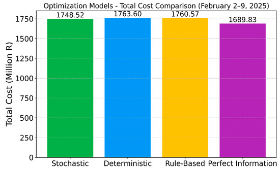
Figure 9.
Total system cost comparison across four optimization models. The Stochastic model achieves a lower cost than the Deterministic and Rule-Based models by accounting for uncertainty and penalizing load shedding. The Perfect Information model represents the theoretical minimum cost.
4.4. Load Shedding and Curtailment Analysis
Figure 10 and Figure 11 present the four models’ ability to manage system reliability over 7 days. The Perfect Information model achieves zero load shedding and curtailment due to its assumption of full foresight, which enables optimal coordination between coal generation, storage, and renewables. In contrast, the Stochastic model, which incorporates multiple forecast scenarios, registers significantly lower penalties (1625 MWh of load shedding and 1283 MWh of curtailment) compared to the Deterministic (3538 MWh and 59 MWh) and Rule-Based (1809 MWh and 1475 MWh) models. These results demonstrate the value of scenario-based optimization in mitigating the impact of variability, even though some supply–demand mismatches remain due to storage and ramping constraints.
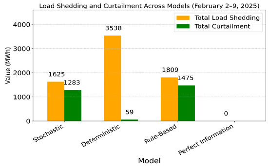
Figure 10.
Total load shedding and curtailment over 7 days.
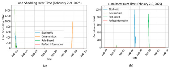
Figure 11.
(a) Daily load shedding (b) curtailment over 7 days.
Temporal analysis over the 7 days reinforces these findings. While the Perfect Information model maintains a flat profile with no violations, the Stochastic model exhibits modest peaks in both load shedding and curtailment, each reaching around 1500 MW and 1000 MW. In contrast, the Deterministic and Rule-Based models record a higher number of load shedding violations, while the Deterministic model has a better curtailment performance than the Stochastic model. Figure 11 and Figure 12 reveal a clear relationship between storage levels and system events such as load shedding and renewable curtailment. On 3 February, all strategies were at a significant battery depletion state in Figure 12, which aligns with the observed load shedding event on the same day. This highlights the system’s inability to meet demand due to insufficient stored energy. Conversely, 6 February was marked by high curtailment levels, as shown in Figure 11b, which are in accordance with the near-maximum battery storage levels shown for the same day in Figure 12a. This suggests that excess renewable generation could not be utilized or stored further. The Deterministic model’s higher load shedding value indicates that it is prone to failure under forecast errors. The Stochastic model strikes a cost-effective compromise between reliability and flexibility, with opportunities for further improvement through enhanced storage and disaggregated renewable modeling.
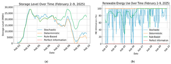
Figure 12.
(a) Storage level over time (b) renewable energy utilization over time.
4.5. Storage and Renewable Utilization over Time
The storage level plot in Figure 12a illustrates notable differences in battery behavior across the four dispatch strategies. The Stochastic approach consistently maintains higher and more stable storage levels until the 8th of February, indicating more effective anticipation of uncertainty and better preservation of battery energy. However, a notable sharp drop in battery storage levels is observed on the 8th day in both the Deterministic and Stochastic models. This can be attributed to the forecast error revealed in Figure 7 on the same day (February 8), and more specifically, an overestimation of demand. This overestimation leads the models to anticipate higher energy consumption, prompting premature or excessive dispatch from the battery. As a result, storage resources are depleted more aggressively than necessary. This effect highlights the vulnerability of forecast-driven dispatch models to systematic prediction biases. The Rule-Based model handles the error better, as seen in Figure 12, primarily due to its conservative and preemptive charging strategy. Unlike Stochastic or Deterministic models that rely heavily on forecasts, which can be inaccurate, the Rule-Based approach prioritizes early charging when excess RE is available, thereby maintaining a consistently higher state of charge. This minimizes the risk of depletion during peak demand periods or forecast errors.
Renewable energy utilization trends further distinguish the effectiveness of the dispatch strategies. The Stochastic model achieves high overall RE usage but exhibits frequent dips and occasional negative values to reflect challenges in managing forecast uncertainty and potential overcommitment of renewables. Despite this variability, it generally maintains strong utilization levels, especially compared to simpler approaches. The Deterministic strategy demonstrates steadier performance with consistently high RE utilization, benefiting from clearer scheduling at the cost of reduced flexibility under real-time variability. The Rule-Based approach maintains moderate performance but lacks the dynamic responsiveness needed for higher efficiency.
4.6. Reserve Sufficiency Evaluation
To ensure operational reliability under uncertainty, the stochastic dispatch model incorporates upward reserve requirements as constraints for each generator and storage unit across all scenarios. Reserve sufficiency is evaluated by analyzing the available spinning reserves relative to forecasted demand and net renewable variability. As shown in Figure 13, the Stochastic model consistently maintained reserve levels within the 9–12% band of hourly demand, aligning with standard operational benchmarks. Reserve allocation reached up to 1530 MW during peak periods and never dropped below 820 MW, indicating strong resilience even during high variability. By contrast, the Deterministic model displayed fluctuating reserve margins, with some hours dipping to as low as 430 MW, which is just 2.5% of demand, which coincided with spikes in load shedding and renewable curtailment. The Rule-Based model fared worse, with an average reserve margin of 710 MW and multiple instances where reserve sufficiency fell below 2% of demand, demonstrating its vulnerability under high uncertainty. The Perfect Information model achieved the best performance, with reserves averaging 12.4% of hourly demand and peaking at 1620 MW, but such performance is infeasible in practical systems. These results confirm that the Stochastic framework delivers a balanced reserve strategy, capturing uncertainty effectively and outperforming both heuristic and deterministic baselines. Its ability to pre-allocate adequate reserves across scenarios significantly reduces reliability risks without incurring excessive operational costs.
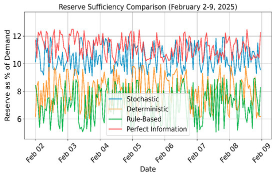
Figure 13.
Reserve sufficiency over 7 days.
4.7. Discussion
Compared to prior work, our approach introduces both methodological innovations and practical improvements in system reliability and uncertainty handling. For example, Zhang et al. [18] utilized a nonparametric KDE-based stochastic optimization framework for a microgrid in Jiangsu, China, but relied on synthetic error modeling instead of forecast-informed scenario generation. In contrast, our study employs empirically trained LSTM–XGBoost models with probabilistic scenario generation derived from real forecast uncertainty, resulting in dispatch strategies that are more aligned with real-world variability. Similarly, Niknami et al. [15] proposed a two-step robust optimization framework for microgrids but did not incorporate probabilistic forecasting or benchmark their results against a range of dispatch strategies. While Mathur et al. [17] implemented Grey Wolf Optimization for dispatch cost minimization in hybrid systems, their focus was limited to islanded microgrid scenarios and heuristic optimization. Our two-stage stochastic MILP model ensures feasibility and near-optimality across multiple uncertainty scenarios and scales to national-level operations using five years of South African energy data. Quantitatively, our stochastic model reduced load shedding by over 50% relative to a deterministic baseline while incurring only a marginal increase in system cost, demonstrating an effective cost-reliability trade-off. This complements the work of Li et al. [16], who employed CVaR for risk-aware microgrid scheduling, although their approach relied heavily on scenario generation via Monte Carlo simulation without integrating forecast-based uncertainty measures. Compared to CVaR-based stochastic optimization, which prioritizes minimizing tail risks beyond a certain quantile, our MILP-based framework offers greater transparency, solver efficiency, and explicit treatment of operational constraints like reserves and curtailment. While CVaR offers value for risk-averse operations, our model strikes a practical balance between risk management and computational tractability for large-scale systems. We acknowledge that more advanced forecasting techniques, such as hierarchical temporal models for solar generation and Bayesian deep learning methods, could further improve uncertainty quantification and forecast calibration. These extensions offer promising future directions for enhancing prediction granularity and probabilistic interpretability, especially in solar forecasting, where sharp daily peaks and intermittency present ongoing challenges.
5. Conclusions
This study presents an optimization framework aimed at enhancing renewable integration by optimizing dispatch under RE uncertainty using South Africa’s power system as a representative case study. A scenario-based stochastic optimization approach is proposed, which integrates machine learning-based forecasting with uncertainty quantification to support more resilient and cost-effective operational planning. Specifically, a hybrid LSTM–XGBoost model is developed to forecast wind, PV, concentrated solar power (CSP), and electricity demand. Monte Carlo dropout and quantile regression techniques are employed to capture uncertainty, and scenarios are generated using appropriate probability distribution models. The optimization framework evaluates four dispatch strategies—Perfect Information, Stochastic, Deterministic, and Rule-Based—under realistic operational constraints and cost penalties for curtailment and load shedding. The Perfect Information model served as a benchmark for ideal system performance with zero load shedding and curtailment. Among the implemented strategies, the Stochastic model demonstrated the highest effectiveness by incorporating multiple future scenarios, thus enabling more balanced and stable system operations. It significantly reduced reliance on non-renewable generation while also minimizing curtailment and load shedding. In contrast, the Deterministic and Rule-Based models were hindered by rigid planning and poor adaptability to uncertainty, resulting in high operational penalties and inefficiencies. This study demonstrates that forecast-informed, probabilistic optimization strategies are critical to managing the complexities of renewable-integrated power systems. With modest increases in computational overhead, such strategies can significantly enhance system resilience, reduce dependence on fossil-based generation, and support a more flexible and cost-effective energy transition. Future research will extend validation across multi-seasonal and multi-year horizons to assess long-term performance. The framework may also be expanded to incorporate DC or AC power flow models, enabling spatially aware dispatch decisions and ensuring voltage stability across the transmission network.
Author Contributions
Conceptualization, M.O.; methodology, M.O.; data analysis, M.O.; validation, M.O. and J.M.; coding, M.O.; writing—original draft preparation, M.O.; review and editing, J.M.; supervision, J.M.; funding acquisition, J.M. All authors have read and agreed to the published version of the manuscript.
Funding
This research and the APC were funded by Tshwane University of Technology, Pretoria, South Africa.
Data Availability Statement
The original contributions presented in this study are included in the article. Further inquiries can be directed to the corresponding author.
Acknowledgments
The authors acknowledge Tshwane University of Technology, Pretoria, South Africa. The corresponding author is grateful to the Management of Olabisi Onabanjo University, Ago Iwoye, Ogun State, Nigeria for granting leave for the research fellowship.
Conflicts of Interest
The authors declare no conflicts of interest.
Abbreviations
| ARIMA | AutoRegressive Integrated Moving Average |
| CSP | Concentrated Solar Power |
| CUR | Curtailment |
| DO | Deterministic Optimization |
| EO | Equilibrium Optimizer |
| GCC | Grid Control Center |
| GWO | Grey Wolf Optimization |
| GWh | Gigawatt-hour |
| KDE | Kernel Density Estimation |
| LS | Load Shedding |
| LSTM | Long Short-Term Memory |
| MC | Monte Carlo |
| MILP | Mixed-Integer Linear Programming |
| ML | Machine Learning |
| MPIW | Mean Prediction Interval Width |
| MW | Megawatt |
| MWh | Megawatt-hour |
| PI | Perfect Information |
| PICP | Prediction Interval Coverage Probability |
| PSO | Particle Swarm Optimization |
| PV | Photovoltaic |
| R | South African Rand |
| RB | Rule-Based |
| RE | Renewable Energy |
| SGP | Scenario Generation Process |
| SO | Stochastic Optimization |
| SOC | State of Charge |
| TAKSR | Temporal-Aware K-Means Scenario Reduction |
| TSC | Total System Cost |
| XGBoost | Extreme Gradient Boosting |
| ZAR | South African Rand |
References
- Adebiyi, A.A.; Moloi, K. Renewable energy source utilization progress in South Africa: A review. Energies 2024, 17, 3487. [Google Scholar] [CrossRef]
- Proctor, D. South Africa Grants Emissions Exemptions to Coal-Fired Plants in Effort to Avoid Blackouts. Power Magazine, 31 March 2025. Available online: https://www.powermag.com/ (accessed on 25 June 2025).
- Makgetla, N.; Patel, M. The Coal Value Chain in South Africa; Trade & Industrial Policy Strategies: Pretoria, South Africa, 2021. [Google Scholar]
- Gautam, S.; Awasthi, A.; Gautam, S.G. Sustainable Air; Springer: Berlin/Heidelberg, Germany, 2024. [Google Scholar]
- Saleh, H.M.; Hassan, A.I. The challenges of sustainable energy transition: A focus on renewable energy. Appl. Chem. Eng. 2024, 7, 2084. [Google Scholar] [CrossRef]
- Zhu, Y.; Li, J.; Liu, P.; Zhang, G.; Liu, H. Modeling and Optimization of an Integrated Energy Supply in the Oil and Gas Industry: A Case Study of Northeast China. Processes 2025, 13, 1512. [Google Scholar] [CrossRef]
- Arévalo, P.; Ochoa-Correa, D.; Villa-Ávila, E. Optimizing Microgrid Operation: Integration of Emerging Technologies and Artificial Intelligence for Energy Efficiency. Electronics 2024, 13, 3754. [Google Scholar] [CrossRef]
- Kumari, P.; Kumar, R. Adaptive virtual inertia-based optimal enhancement of micro-grid dynamics with integrated renewable energy sources. Int. J. Ambient Energy 2025, 46, 2456762. [Google Scholar] [CrossRef]
- Aljarrah, R.; Fawaz, B.B.; Salem, Q.; Karimi, M.; Marzooghi, H.; Azizipanah-Abarghooee, R. Issues and challenges of grid-following converters interfacing renewable energy sources in low inertia systems: A review. IEEE Access 2024, 12, 5534–5561. [Google Scholar] [CrossRef]
- Rahman, K.; Hashimoto, J.; Orihara, D.; Ustun, T.S.; Otani, K.; Kikusato, H.; Kodama, Y. Reviewing control paradigms and emerging trends of grid-forming inverters—A comparative study. Energies 2024, 17, 2400. [Google Scholar] [CrossRef]
- Khan, M.R.; Haider, Z.M.; Malik, F.H.; Almasoudi, F.M.; Alatawi, K.S.S.; Bhutta, M.S. A Comprehensive Review of Microgrid Energy Management Strategies Considering Electric Vehicles, Energy Storage Systems, and AI Techniques. Processes 2024, 12, 270. [Google Scholar] [CrossRef]
- Singh, S.; Singh, S. Advancements and challenges in integrating renewable energy sources into distribution grid systems: A comprehensive review. J. Energy Resour. Technol. 2024, 146, 090801. [Google Scholar] [CrossRef]
- Saleeb, H.; El-Rifaie, A.M.; Sayed, K.; Accouche, O.; Mohamed, S.A.; Kassem, R. Optimal Sizing and Techno-Economic Feasibility of Hybrid Microgrid. Processes 2025, 13, 1209. [Google Scholar] [CrossRef]
- Ramadan, A.; Ebeed, M.; Kamel, S.; Abdelaziz, A.Y.; Haes Alhelou, H. Scenario-based stochastic framework for optimal planning of distribution systems including renewable-based dg units. Sustainability 2021, 13, 3566. [Google Scholar] [CrossRef]
- Niknami, A.; Askari, M.T.; Ahmadi, M.A.; Nik, M.B.; Moghaddam, M.S. Resilient day-ahead microgrid energy management with uncertain demand, EVs, storage, and renewables. Clean. Eng. Technol. 2024, 20, 100763. [Google Scholar] [CrossRef]
- Li, K.; Yang, F.; Wang, L.; Yan, Y.; Wang, H.; Zhang, C. A scenario-based two-stage stochastic optimization approach for multi-energy microgrids. Appl. Energy 2022, 322, 119388. [Google Scholar] [CrossRef]
- Mathur, A.; Kumari, R.; Meena, V.; Singh, V.; Azar, A.T.; Hameed, I.A. Data-driven optimization for microgrid control under distributed energy resource variability. Sci. Rep. 2024, 14, 10806. [Google Scholar] [CrossRef] [PubMed]
- Zhang, D.; Jiang, S.; Liu, J.; Wang, L.; Chen, Y.; Xiao, Y.; Jiao, S.; Xie, Y.; Zhang, Y.; Li, M. Stochastic Optimization Operation of the Integrated Energy System Based on a Novel Scenario Generation Method. Processes 2022, 10, 330. [Google Scholar] [CrossRef]
- Abdelghany, M.B.; Al-Durra, A.; Zeineldin, H.; Gao, F. Integrating scenario-based stochastic-model predictive control and load forecasting for energy management of grid-connected hybrid energy storage systems. Int. J. Hydrogen Energy 2023, 48, 35624–35638. [Google Scholar] [CrossRef]
- Gu, Z.; Li, B.; Zhang, G. Optimizing photovoltaic integration in grid management via a deep learning-based scenario analysis. Sci. Rep. 2025, 15, 14851. [Google Scholar] [CrossRef]
- Sakib, T.H. Probabilistic Modeling of Source and Load Uncertainties for Optimal Sizing of Hybrid Renewable Energy System. Ph.D. Thesis, Department of Electrical and Elecrtonics Engineering (EEE), Islamic University of Technology (IUT), Gazipur, Bangladesh, 2024. [Google Scholar]
- Al-Lawati, R.A.; Faiz, T.I.; Noor-E-Alam, M. A nationwide multi-location multi-resource stochastic programming based energy planning framework. Energy 2024, 295, 130898. [Google Scholar] [CrossRef]
- Eskom. South Africa Energy Generation and Demand Data; Eskom: Sandton, South Africa, 2025. [Google Scholar]
- Climate Information Portal. Weather Data; Climate System Analysis Group, University of Cape Town, South Africa, 2020. Available online: https://cip.csag.uct.ac.za/webclient2/app/#datasets (accessed on 25 June 2025).
- Hyndman, R.J.; Athanasopoulos, G. Forecasting: Principles and Practice; OTexts: Melbourne, Australia, 2018. [Google Scholar]
- Sarmas, E.; Marinakis, V.; Doukas, H. Deep Learning Models for Short-Term Forecasting of Photovoltaic Energy Production. In Artificial Intelligence for Energy Systems: Driving Intelligent, Flexible and Optimal Energy Management; Springer Nature: Cham, Switzerland, 2025; pp. 87–127. [Google Scholar]
- Goodfellow, I.; Bengio, Y.; Courville, A.; Bengio, Y. Deep Learning; MIT Press: Cambridge, MA, USA, 2016; Volume 1. [Google Scholar]
- Suebsombut, P.; Sekhari, A.; Sureephong, P.; Belhi, A.; Bouras, A. Field data forecasting using LSTM and Bi-LSTM approaches. Appl. Sci. 2021, 11, 11820. [Google Scholar] [CrossRef]
- Durand, D.; Aguilar, J.; R-Moreno, M.D. An analysis of the energy consumption forecasting problem in smart buildings using LSTM. Sustainability 2022, 14, 13358. [Google Scholar] [CrossRef]
- Masood, Z.; Gantassi, R.; Choi, Y. A multi-step time-series clustering-based Seq2Seq LSTM learning for a single household electricity load forecasting. Energies 2022, 15, 2623. [Google Scholar] [CrossRef]
- Lei, P.; Ma, F.; Zhu, C.; Li, T. LSTM short-term wind power prediction method based on data preprocessing and variational modal decomposition for soft sensors. Sensors 2024, 24, 2521. [Google Scholar] [CrossRef] [PubMed]
- Shering, T.; Alonso, E.; Apostolopoulou, D. Investigation of load, solar and wind generation as target variables in LSTM Time Series forecasting, using exogenous Weather variables. Energies 2024, 17, 1827. [Google Scholar] [CrossRef]
- Alonso, A.M.; Nogales, F.J.; Ruiz, C. A single scalable LSTM model for short-term forecasting of massive electricity time series. Energies 2020, 13, 5328. [Google Scholar] [CrossRef]
- Moon, Y.; Lee, Y.; Hwang, Y.; Jeong, J. Long Short-Term Memory Autoencoder and Extreme Gradient Boosting-Based Factory Energy Management Framework for Power Consumption Forecasting. Energies 2024, 17, 3666. [Google Scholar] [CrossRef]
- Van Houdt, G.; Mosquera, C.; Nápoles, G. A review on the long short-term memory model. Artif. Intell. Rev. 2020, 53, 5929–5955. [Google Scholar] [CrossRef]
- Ke, G.; Meng, Q.; Finley, T.; Wang, T.; Chen, W.; Ma, W.; Ye, Q.; Liu, T.-Y. Lightgbm: A highly efficient gradient boosting decision tree. In Proceedings of the Advances in Neural Information Processing Systems, Long Beach, CA, USA, 4–9 December 2017; Volume 30. [Google Scholar]
- Wang, T.; Liu, H.; Su, M. Energy Optimization for Microgrids Based on Uncertainty-Aware Deep Deterministic Policy Gradient. Processes 2025, 13, 1047. [Google Scholar] [CrossRef]
- Mdee, O.J. Performance evaluation of Weibull analytical methods using several empirical methods for predicting wind speed distribution. Energy Sources Part A Recovery Util. Environ. Eff. 2025, 47, 1626–1649. [Google Scholar] [CrossRef]
- Fernandez-Jimenez, L.A.; Monteiro, C.; Ramirez-Rosado, I.J. Short-term probabilistic forecasting models using Beta distributions for photovoltaic plants. Energy Rep. 2023, 9, 495–502. [Google Scholar] [CrossRef]
- Salmerón-Gómez, R.; García-García, C.B.; García-Pérez, J. A redefined variance inflation factor: Overcoming the limitations of the variance inflation factor. Comput. Econ. 2025, 65, 337–363. [Google Scholar] [CrossRef]
- Maisano, J.; Radchik, A.; Ling, T. A lognormal model for demand forecasting in the national electricity market. ANZIAM J. 2016, 57, 369–383. [Google Scholar]
- Gao, S.; Wang, Y.; Zhou, Y.; Yu, H. An Improved Scheduling Approach for Multi-Energy Microgrids Considering Scenario Insufficiency and Computational Complexity. Processes 2025, 13, 576. [Google Scholar] [CrossRef]
- Fei, N.; Gao, Y.; Lu, Z.; Xiang, T. Z-score normalization, hubness, and few-shot learning. In Proceedings of the IEEE/CVF International Conference on Computer Vision, Montreal, BC, Canada, 11–17 October 2021; pp. 142–151. [Google Scholar]
- Lai, H.; Huang, T.; Lu, B.; Zhang, S.; Xiaog, R. Silhouette coefficient-based weighting k-means algorithm. Neural Comput. Appl. 2025, 37, 3061–3075. [Google Scholar] [CrossRef]
- Azevedo, B.F.; Rocha, A.M.A.; Pereira, A.I. A multi-objective clustering algorithm integrating intra-clustering and inter-clustering measures. In Proceedings of the International Conference on Optimization and Learning, Dubrovnik, Croatia, 13–15 May 2024; Springer: Berlin/Heidelberg, Germany, 2024. [Google Scholar]
- Anand, R.; Aggarwal, D.; Kumar, V. A comparative analysis of optimization solvers. J. Stat. Manag. Syst. 2017, 20, 623–635. [Google Scholar] [CrossRef]
- Eskom. Tariffs and Charges. Available online: https://www.eskom.co.za/distribution/tariffs-and-charges/ (accessed on 12 July 2025).
- Manyane, T.; Nembahe, R. South African Energy Price Report 2024; Department of Mineral Resources and Energy: Pretoria, South Africa, 2025.
- Hodson, T.O. Root mean square error (RMSE) or mean absolute error (MAE): When to use them or not. Geosci. Model Dev. Discuss. 2022, 15, 5481–5487. [Google Scholar] [CrossRef]


Disclaimer/Publisher’s Note: The statements, opinions and data contained in all publications are solely those of the individual author(s) and contributor(s) and not of MDPI and/or the editor(s). MDPI and/or the editor(s) disclaim responsibility for any injury to people or property resulting from any ideas, methods, instructions or products referred to in the content. |
© 2025 by the authors. Licensee MDPI, Basel, Switzerland. This article is an open access article distributed under the terms and conditions of the Creative Commons Attribution (CC BY) license (https://creativecommons.org/licenses/by/4.0/).