Short-Term Wind Power Forecasting Based on Improved Modal Decomposition and Deep Learning

Abstract

With the continued growth in wind power installed capacity and electricity generation, accurate wind power forecasting has become increasingly critical for power system stability and economic operations. Currently, short-term wind power forecasting often employs deep learning models following modal decomposition of wind power time series. However, the optimal length of the time series used for decomposition remains unclear. To address this issue, this paper proposes a short-term wind power forecasting method that integrates improved modal decomposition with deep learning techniques. First, the historical wind power series is segmented using the Pruned Exact Linear Time (PELT) method. Next, the segmented series is decomposed using an enhanced Complete Ensemble Empirical Mode Decomposition with Adaptive Noise (ICEEMDAN) to extract multiple modal components. High-frequency oscillatory components are then further decomposed using Variational Mode Decomposition (VMD), and the resulting modes are clustered using the K-means algorithm. The reconstructed components are subsequently input into a Long Short-Term Memory (LSTM) network for prediction, and the final forecast is obtained by aggregating the outputs of the individual modes. The proposed method is validated using historical wind power data from a wind farm. Experimental results demonstrate that this approach enhances forecasting accuracy, supports grid power balance, and increases the economic benefits for wind farm operators in electricity markets.

1. Introduction

Since fossil fuels are non-renewable and their consumption leads to significant environmental pollution, there is an urgent need to replace them with renewable and environmentally friendly energy sources, supraduction as wind energy. Wind power generation offers several advantages: it is pollution-free, renewable, and economically viable. In recent years, China’s electricity demand and installed power generation capacity have continued to grow, accelerating the nation’s transition to clean energy. As a result, the scale of renewable energy—particularly wind power—has expanded rapidly. By the end of December 2024, China’s cumulative installed power generation capacity reached approximately 3.35 billion kilowatts, representing a year-on-year increase of 14.6%. Among this, wind power accounted for around 520 million kilowatts, an 18.0% increase compared to the previous year [1]. As both total and wind-specific installed capacities continue to rise, wind power forecasting plays an increasingly vital role in power system management and economic operations. However, the high volatility and unpredictability of wind speed pose considerable challenges to power system stability and market efficiency. Therefore, accurate wind power forecasting is crucial for grid scheduling, maintaining system reliability, and improving the economic returns for wind farm operators [2]. From the perspective of modeling approaches, wind power forecasting methods are generally classified into three categories: physical models, time series models, and artificial intelligence-based models [3].

The physical modeling approach to wind power forecasting primarily relies on Numerical Weather Prediction (NWP) techniques [4]. This method uses real-time meteorological observations and terrain features as initial boundary conditions to construct a three-dimensional atmospheric model. By solving fluid dynamics and thermodynamic equations, it simulates the spatial and temporal distribution of wind speed and direction at the hub height of wind turbines. These simulated meteorological parameters are then converted into theoretical power output using the specific power curve of a given wind farm. Reference [5] introduced an integrated approach that combines the outputs of three different meteorological models. By analyzing the covariance matrix of prediction deviations and errors from individual models, optimal weights are determined to enhance forecasting accuracy. Reference [6] proposed a short-term wind speed forecasting method that precomputes discrete boundary conditions and utilizes a flow field characteristics database for interpolation, thereby estimating wind speed and direction under specific scenarios. To address the limitations of low-resolution NWP data, Reference [7] analyzed the influence of terrain and wake effects on wind flow using fluid mechanics principles, leading to more accurate predictions. Despite their strengths, physical models face several application limitations in wind power forecasting. They are highly sensitive to the accuracy of input data—particularly meteorological and terrain parameters—and are vulnerable to environmental disturbances. Moreover, these models typically have limited generalizability when applied to different sites. From a computational perspective, solving the underlying fluid mechanics equations requires substantial computing resources and time, making this approach computationally intensive. Additionally, forecasting errors tend to accumulate over longer prediction horizons, which reduces the reliability of physical models in short-term forecasting tasks. However, physical modeling methods exhibit better performance in medium- to long-term forecasting scenarios, particularly in strategic applications such as site selection, wind resource assessment, and long-term energy planning [8,9].

In recent years, research has increasingly focused on the practical demands of power load forecasting and renewable energy modeling, conducting in-depth analyses of the applicability of traditional modeling approaches in complex scenarios. Reference [10] reported that, in short-term load forecasting experiments during the Easter holiday in Italy, the accuracy of traditional statistical models dropped significantly due to increased volatility during the holiday period, making them inadequate for capturing abrupt fluctuations in demand. Increment (2021) further pointed out that as the forecasting horizon and input data complexity increase, the linear modeling capability of conventional time series methods gradually falls short of the precision requirements in modern energy systems, necessitating the adoption of more expressive machine learning approaches. Reference [11] also emphasized that in hourly load estimation under a 100% renewable energy scenario, the non-stationary and intermittent nature of wind and solar power poses serious challenges to classical time series models, thus highlighting the urgent need for high-resolution nonlinear modeling frameworks to enhance model adaptability and robustness.

Time series forecasting models predict future trends by analyzing the temporal patterns embedded in historical data. Among these methods, the persistence model is the simplest and most straightforward strategy, which assumes that the value observed at the current time step will remain unchanged in the next. More sophisticated models include the Autoregressive (AR) model [12], Moving Average (MA) model [13], Autoregressive Moving Average (ARMA) model [14], and Autoregressive Integrated Moving Average (ARIMA) model [15]. Each of these methods employs distinct mathematical formulations to capture the dynamics of time series data and improve forecasting accuracy. For instance, Reference [16] applied time series analysis techniques to develop a wind speed prediction model for wind farms. Further, studies have shown that employing an improved ARMA model can significantly enhance the accuracy of short- and medium-term wind power forecasts [17]. However, traditional time series models have several intrinsic limitations. First, these methods typically assume that the input data are stationary. When applied to inherently non-stationary wind power data, their predictive accuracy tends to deteriorate significantly. Second, while these models are effective in capturing linear dependencies, they struggle to model the complex nonlinear interactions that often exist in real-world wind power data. Third, such models are generally better suited for static environments and may underperform in scenarios where data exhibit dynamic and evolving patterns. Notably, when applied to time series with complex characteristics, the limitations of traditional single-model approaches in feature extraction and representation become increasingly pronounced, making it difficult to meet the growing demands for high-accuracy wind power forecasting.

Single-model forecasting approaches often struggle to fully capture the complex dynamic characteristics of wind power data, which exhibit strong nonlinearity and multi-scale fluctuations, thereby limiting their predictive performance. To address this limitation, researchers in recent years have increasingly turned to multi-model fusion strategies, which integrate the structural advantages of different models. This approach has gradually become the mainstream trend in wind power forecasting research. Combined models not only significantly improve prediction accuracy but also enhance model stability and generalization ability. For example, reference [18] proposed an improved artificial neural network model that incorporates particle swarm optimization (PSO) and genetic algorithm (GA) for joint parameter optimization, effectively improving convergence speed and forecast accuracy. Reference [19] developed a deep neural network that combines wavelet transform with a Transformer architecture, demonstrating excellent multivariate time series modeling capabilities and achieving high-precision prediction of wind speed and power. Moreover, reference [20] proposed a hybrid forecasting system that integrates LSTM and Transformer frameworks to jointly model the power generation process of wind, solar, and battery storage systems, thereby significantly improving the prediction reliability and practical applicability of renewable energy systems.

With the continuous advancement of artificial intelligence (AI) technologies, a wide range of statistical methods based on intelligent learning have emerged, among which machine learning has seen particularly extensive application. As a key branch of AI, machine learning models can adaptively learn from existing data to optimize decision-making and predict future or unseen scenarios, thereby enhancing both accuracy and generalizability [21]. Commonly used machine learning algorithms in wind power and wind speed forecasting include regression models, Support Vector Machines (SVMs), Random Forests (RFs), Bayesian Additive Regression Trees (BARTs), and K-Nearest Neighbors (KNNs). These algorithms have demonstrated strong capabilities in capturing complex patterns in meteorological and power generation data. In recent years, the rapid development of deep learning has driven significant breakthroughs in artificial intelligence, particularly in domains such as speech recognition and computer vision. This technological wave has also profoundly influenced the field of wind power forecasting. For example, Reference [22] proposed a hybrid method combining Empirical Mode Decomposition (EMD) with Artificial Neural Networks (ANN) for wind power prediction. Reference [23] applied an improved Variational Mode Decomposition (VMD) to preprocess wind power data and employed a Long Short-Term Memory (LSTM) network for forecasting, significantly enhancing prediction accuracy. These studies introduced innovative data processing and modeling strategies aimed at improving both the precision and robustness of wind power forecasting. Furthermore, Reference [24] developed a hybrid LSTM–SARIMA model for ultra-short-term wind power forecasting, integrating LSTM with the Seasonal Autoregressive Integrated Moving Average (SARIMA) model. This approach accounts for both meteorological and seasonal variations, effectively capturing wind power fluctuations and improving upon the limitations of traditional models. Reference [25] presented a comprehensive energy load forecasting framework based on hybrid mode decomposition and deep learning. The framework adopts a multi-stage decomposition strategy: initially, Complete Ensemble Empirical Mode Decomposition with Adaptive Noise (CEEMDAN) is applied to disaggregate the electricity, cooling, and heating load data into intrinsic mode components. For components exhibiting significant residual non-stationarity, VMD is subsequently used for secondary refinement.

Existing research has demonstrated that decomposing historical wind power time series prior to forecasting can significantly improve prediction accuracy. Modal decomposition techniques enable the extraction of intrinsic components from complex signals, helping to uncover latent patterns and improve model performance. These techniques are particularly well-suited to nonlinear and non-stationary signals, offering benefits such as noise reduction, enhanced data preprocessing, and improved predictive capabilities. Moreover, modal decomposition facilitates a deeper understanding of signal characteristics, thereby enhancing the quality of time series analysis. For these reasons, it has been widely adopted in wind power forecasting and related fields. Compared with conventional forecasting methods, decomposition-based hybrid models offer a relatively simple structure, high computational efficiency, and strong adaptability. Such models can be effectively applied to various forecasting scenarios, including point forecasts, multi-step forecasts, and day-ahead predictions. However, a notable limitation of current decomposition-prediction models is the lack of clear guidance on determining the appropriate length of the time series segment to be decomposed. The choice of time window length can significantly influence the quality of decomposition and, consequently, the accuracy of the final forecast. Despite its importance, this issue remains insufficiently addressed in existing studies. Therefore, there is an urgent need for further research to explore and optimize time series segmentation strategies in the context of decomposition-based wind power forecasting.

Based on the above background, this paper proposes a short-term wind power forecasting method that integrates improved modal decomposition with deep learning, aiming to address the challenge of determining the appropriate length of time series for decomposition. The main contributions of this study are summarized as follows:

(1) A novel forecasting framework is proposed that combines improved modal decomposition with deep learning to enhance short-term wind power prediction. The method adopts a multi-stage processing strategy for historical wind power data to improve forecasting accuracy.

(2) Time series segmentation is performed prior to modal decomposition using the Pruned Exact Linear Time (PELT) method, enabling precise determination of the optimal time series length. A two-stage modal decomposition process is then applied: the first stage reduces noise and complexity, while the second targets high-frequency oscillatory components to further refine the decomposition and simplify prediction.

(3) K-means clustering is employed after decomposition to group similar modal components. This not only reduces computational cost but also leverages shared characteristics among components, improving efficiency and prediction performance.

2. Introduction to Related Theories

2.1. Improved Modal Decomposition

2.1.1. PELT-Mean &Variance

The Pruned Exact Linear Time (PELT) algorithm is a widely used technique for detecting change points in time series data. It is particularly effective for identifying segments in datasets that exhibit abrupt shifts in statistical properties such as the mean and variance. PELT operates by optimizing a cost function that incorporates a goodness-of-fit term and a penalty for the number of change points, thereby avoiding over-segmentation while ensuring accurate detection. One of the key advantages of PELT is its computational efficiency, achieved by pruning suboptimal candidate change points during the search process. This enables the algorithm to provide a globally optimal segmentation in linear time under certain conditions, making it highly suitable for large-scale and high-frequency time series data, such as wind power generation. Among the various formulations of PELT, the PELT-Mean &Variance model is particularly well-suited for wind power data due to the inherent high volatility and fluctuations in both the mean and variance of the signal. This version of the algorithm is designed to detect change points where either or both of these statistical properties shift significantly over time. The formula is as follows:

$$C(\tau )={\displaystyle \sum _{i=0}^m\left[{\displaystyle \sum _{t={\tau }_i+1}^{{\tau }_{i+1}}{(X_t-{\mu }_i)}^2}+{\displaystyle \sum _{t={\tau }_i+1}^{{\tau }_{i+1}}\frac{{(X_t-{\mu }_i)}^2}{{\sigma }_i^2}+\beta }\right]}$$

(1)

where: $C(\tau )$ is the total cost function, representing the objective function that is minimized to identify the optimal change points. It is calculated as the sum of the segment costs for all detected segments plus a penalty term. ${\displaystyle \sum _{i=0}^m}$ denotes the summation over all segments in the time series. The number of segments is m + 1, where m is the number of change points, and each segment is indexed by i. $\tau =\{{\tau }_1,{\tau }_2,\dots ,{\tau }_m\}$ represents the set of change points. Each change point in ${\tau }_1,{\tau }_2,\dots ,{\tau }_m$ divides the time series into multiple segments. ${\displaystyle \sum _{t={\tau }_i+1}^{{\tau }_{i+1}}{(X_t-{\mu }_i)}^2}$ is the segment cost, typically calculated as the sum of the variance of the mean. It measures how well the segment mean represents the observed values in that segment. $X_t$ is the observed wind power value at time t. ${\mu }_i$ is the mean estimate for the segment containing time t. ${(X_t-{\mu }_i)}^2$ is the variance for a single observation, measuring the deviation of each observed value from the segment mean.${\mu }_i={\displaystyle \frac{1}{{\tau }_{i+1}-{\tau }_i}}{\displaystyle \sum _{{\tau }_i+1}^{{\tau }_{i+1}}{X}_t}$ is the mean of segment i, calculated as the average wind power across all time points in the segment. ${\displaystyle \sum _{t={\tau }_i+1}^{{\tau }_{i+1}}\frac{{(X_t-{\mu }_i)}^2}{{\sigma }_i^2}}$ is the variance penalty term, used to account for the spread of the data within the segment. ${\sigma }_i^2$ is the variance estimate for segment i.${\displaystyle \frac{{(X_t-{\mu }_i)}^2}{{\sigma }_i^2}}$ normalizes the variance by the segment’s variance. Summing across all time points in a segment ensures that segments with higher variance contribute more to the cost. ${\sigma }_i^2={\displaystyle \frac{1}{{\tau }_{i+1}-{\tau }_i}}{\displaystyle \sum _{t={\tau }_i+1}^{{\tau }_{i+1}}{(X_t-{\mu }_i)}^2}$ is the variance of segment i, which quantifies the dispersion of wind power values from the segment mean. A larger variance indicates greater fluctuation within the segment. $\beta$ is the penalty term for introducing a change point. It regulates the total number of change points: a larger $\beta$ discourages over-segmentation and leads to smoother partitions, while a smaller $\beta$ allows for more detailed segmentation, which can better capture rapid fluctuations in wind power data.

2.1.2. ICEEMDAN

The Improved Complete Ensemble Empirical Mode Decomposition with Adaptive Noise (ICEEMDAN) is an enhanced signal decomposition method derived from the fully adaptive noise-based Complete Ensemble Empirical Mode Decomposition (CEEMDAN) [26]. It aims to further overcome the limitations of both the traditional Empirical Mode Decomposition (EMD) and CEEMDAN. When dealing with non-stationary signals, EMD often suffers from mode mixing—where components of different frequencies are present in the same intrinsic mode function (IMF)—leading to ambiguous and unstable time-frequency representations. Additionally, EMD is sensitive to noise and boundary effects. While CEEMDAN alleviates some mode mixing by adding white noise, it still introduces redundant information at each decomposition layer, potentially obscuring weak signal components.

The core idea of ICEEMDAN is to integrate white noise with the original signal and inject it step-by-step during decomposition. This strategy improves frequency separation, suppresses mode mixing, and enhances the stability and accuracy of the decomposition process. ICEEMDAN employs an adaptive noise-injection mechanism in each IMF extraction stage, introducing specific amounts of white noise and performing EMD to extract the corresponding oscillatory mode. A set of independent white noise sequences $w^{(i)}$ is first generated to enrich the frequency response of the original signal $x$. For each noise realization, the first-order mode component $E_1\left(w^{(i)}\right)$ is extracted using EMD, scaled appropriately, and added to the original signal to form a perturbed version $x^{(i)}$:

$$x^{(i)}=x+{\beta }_0{E}_1(w^{(i)})$$

(2)

where ${\beta }_0={\epsilon }_{0}std(x)/std(E_1(w^{(i)}))$ is the inverse of the required SNR between the first added noise and the analysis signal, expressing the SNR as the quotient of the standard deviation; $E_{\mathrm{k}}(·)$ is the k-order modal component generated by EMD decomposition; $w^{(i)}$ represents the i-th group of white noise used to assist decomposition; When k is greater than or equal to 1, ${\beta }_k={\epsilon }_{0}std(r_k)$; $x^{(i)}$.

Next, the local mean of each perturbed signal $x^{(i)}$ is computed as follows:

$$r_1=\langle M(x^{(i)})\rangle$$

(3)

where $x^{(i)}$ is the wind power time series after adding the i-th group of special noise; $M(·)$ is an operator that generates the local mean of the signal. In the first stage (k = 1), the first mode is calculated:

$$d_1=x-r_1$$

(4)

To extract the second IMF, a new round of noise injection is applied to the residual $r_1$. For each noise realization $w^{(i)}$, the second-order mode $E_2\left(w^{(i)}\right)$ is obtained via EMD. The noise amplitude is adjusted based on the standard deviation of $r_1$, i.e., ${\beta }_1={\epsilon }_0\cdot \mathrm{std}\left(r_1\right)$. Then, by adding the scaled noise to $r_1$ and computing the local mean, the second IMF is derived as follows:

$$d_2=r_1-r_2=r_1-\langle M(r_1+{\beta }_1{E}_2(w^{(i)}))\rangle$$

(5)

In general, for the $k$-th decomposition layer, the residual $r_k$ is calculated as follows:

$$r_k=\langle M(r_{k-1}+{\beta }_{k-1}{E}_k(w^{(i)}))\rangle$$

(6)

and the corresponding $k$-th IMF is obtained by the following:

$$d_k=r_{k-1}-r_k$$

(7)

In these expressions, ${\beta }_k={\epsilon }_0\cdot \mathrm{std}\left(r_k\right)$ ensures that the injected noise remains proportional to the signal at each stage. This self-adjusting mechanism enables the decomposition to preserve the physical significance and scale of each IMF while minimizing interference between frequency bands.

The iteration continues until the final residual $r_K$ no longer exhibits significant oscillatory behavior and is considered the non-oscillatory trend of the signal. At that point, the original signal can be reconstructed as the sum of all IMFs and the final residual:

$$x={\displaystyle \sum _{k=1}^K{d}_k}+r_K$$

(8)

This formulation ensures that ICEEMDAN is complete and lossless, maintaining all the energy content of the original signal and providing a reliable foundation for further feature extraction and analysis.

2.1.3. VMD

To enhance the modeling accuracy of high-frequency components in wind power time series, this study employs a hybrid decomposition approach that combines ICEEMDAN and Variational Mode Decomposition (VMD). ICEEMDAN is effective in suppressing mode mixing and improving the overall smoothness of decomposed components. However, its first IMF (IMF1) often contains high-frequency noise or transient oscillations, which can negatively affect forecasting stability. VMD is thus applied to IMF1 to further refine the component into narrowband, low-correlation sub-signals. This cascaded strategy has been widely supported in recent studies, where multi-level signal decomposition enhances data stationarity and feature representation before feeding into learning models [27,28].

Since the IMF1 component generated by ICEEMDAN decomposition represents a high-frequency oscillation, it is further decomposed using Variational Mode Decomposition (VMD). VMD is a fully non-recursive signal processing method that adaptively determines the center frequency and bandwidth of each mode based on the characteristics of the original signal, generating reliable subsequences with improved interpretability [29]. Compared with the traditional empirical mode decomposition (EMD) method, VMD not only addresses issues such as endpoint effects and modal aliasing but also offers a more rigorous theoretical foundation. This method significantly reduces the non-stationarity of time series data and produces subsequences with distinct frequencies and high stationarity, making it particularly suitable for analyzing complex load series such as wind power generation data. The core principle of VMD involves formulating and solving a variational problem. When constructing this variational problem, it is assumed that the original signal can be decomposed into multiple subsequences, subject to three essential conditions: first, each subsequence must possess a specific center frequency and limited bandwidth; second, the sum of all estimated bandwidths across these subsequences must be minimized; third, the superposition of all modal components must exactly reconstruct the original signal. By satisfying these conditions, VMD achieves an optimal balance between decomposition accuracy and signal fidelity, offering a powerful tool for preprocessing in wind power forecasting and related applications. The mathematical description is as follows:

$$\underset{\left\{u_k\right\},\left\{{\omega }_k\right\}}{\min }\left\{{\displaystyle \sum _k{‖{\partial }_t\left[\left(\delta \left(t\right)+\frac{j}{\pi t}\right)\ast u_k\left(t\right)\right]e^{-j{\omega }_{k}t}‖}_2^2}\right\}$$

(9)

$$s.t.{\displaystyle \sum _{k=1}^K{u}_k\left(t\right)}=f\left(t\right)$$

(10)

where $K$ represents the number of components obtained; $u_k$ and ${\omega }_k$ represent the kth subsequence and the center frequency; $\delta (t)$ represents the Dirac function; and $\ast$ represents the convolution operator.

Solving the above equation and adding the Lagrange multiplication operator, the constrained variation problem is transformed into an unconstrained variation problem, and the following augmented Lagrange formula is obtained:

$$\begin{array}{l}L\left(\left\{u_k\right\},\left\{{\omega }_k\right\},\lambda \right)=\alpha {\displaystyle \sum _k{‖{\partial }_t\left[\left(\delta \left(t\right)+\frac{j}{\pi t}\right)u_k\left(t\right)\right]+e^{-j{\omega }_{k}t}‖}_2^2+}\\ {‖f\left(t\right)-{\displaystyle \sum _k{u}_k\left(t\right)}‖}_2^2+〈\lambda \left(t\right),f\left(t\right)-{\displaystyle \sum _k{u}_k\left(t\right)}〉\end{array}$$

(11)

where $\alpha$ represents the quadratic penalty factor, which is used to reduce the interference from Gaussian noise.

With the help of the alternating direction multiplier iteration algorithm, supplemented by the Pasaval theorem and the Fourier isometric transform, the modal components and center frequencies are obtained, and the saddle points of the augmented Lagrangian function are captured. The alternating optimization iteration formula of $u_k$, ${\omega }_k$, and $\lambda$ is as follows:

$${\widehat{u}}_k^{n+1}(\omega )={\displaystyle \frac{\widehat{f}\left(\omega \right)-{\displaystyle \sum _{i\ne k}{\widehat{u}}_i\left(\omega \right)+\frac{\widehat{\lambda }\left(\omega \right)}{2}}}{1+2\alpha {\left(\omega -{\omega }_k\right)}^2}}$$

(12)

$${\omega }_k^{n+1}={\displaystyle \frac{{\displaystyle {\int }_0^{\infty }\omega {\left|{\widehat{u}}_k\left(\omega \right)\right|}^{2}d\omega }}{{\displaystyle {\int }_0^{\infty }{\left|{\widehat{u}}_k\left(\omega \right)\right|}^{2}d\omega }}}$$

(13)

$${\widehat{\lambda }}^{n+1}(\omega )={\widehat{\lambda }}^n(\omega )+\gamma (f(\omega )-{\displaystyle \sum _k{\widehat{u}}_k^{n+1}(\omega )})$$

(14)

where $\gamma$ represents the noise tolerance, which is used to constrain the fidelity of signal decomposition; ${\widehat{u}}_k^{n+1}(\omega )$, ${\widehat{u}}_i(\omega )$, $f(\omega )$ and $\widehat{\lambda }(\omega )$ are obtained by the Fourier transform of $u_k^{n+1}(t)$, $u_i(t)$, $f(t)$, and $\lambda (t)$.

2.1.4. K-Means Clustering

To enhance the modeling efficiency and forecasting accuracy, this study introduces a dimensionality reduction and clustering mechanism following modal decomposition (e.g., ICEEMDAN or VMD). Since the decomposed intrinsic mode functions (IMFs) often exhibit significant redundancy and overlap in their frequency or temporal structures, directly feeding them into an LSTM network may lead to high input dimensionality, reduced training efficiency, and even overfitting risks.

To address these issues, we first apply Principal Component Analysis (PCA) to the set of decomposed IMF components. PCA identifies the most informative linear projection directions through eigenvalue decomposition, allowing the retention of major signal information while compressing dimensionality. In this study, the number of principal components is determined based on the cumulative contribution rate, preserving at least 95% of the original information. Furthermore, a scree plot is employed to visualize the explained variance of each component and to identify the optimal cut-off point, which also helps assess the clustering potential of the transformed feature space.

Subsequently, the K-means clustering algorithm [30] is applied in the reduced-dimensional feature space to group structurally similar IMF components in an unsupervised manner. This process aims to compress redundant information and abstract representative dynamic structures. The number of clusters is selected using two widely adopted criteria, the Elbow Method and the Silhouette Coefficient, which together ensure a good balance between intra-cluster compactness and inter-cluster separability. This strategy not only reduces the complexity of model inputs but also enhances the clarity of structural features, allowing the LSTM model to focus on more representative dynamic patterns.

By combining PCA and K-means, the proposed framework effectively suppresses redundancy, improves training efficiency, and enhances generalization. Moreover, through its iterative optimization process, K-means identifies the optimal cluster structure that best captures the intrinsic patterns within the data, making it broadly applicable to tasks such as feature extraction, data preprocessing, and model simplification across various fields, including wind power forecasting.

$$J={\displaystyle \sum _{i=1}^k{\displaystyle \sum _{x\in C_i}‖x{-u_i‖}^2}}$$

(15)

where J is the objective function value, which represents the sum of squared errors within the cluster. k is the number of clusters (predefined value). x is a data point in the dataset. $C_i$ is the set of the i-th cluster, which contains all the data points belonging to the cluster. $u_i$ is the centroid (cluster center) of the i-th cluster. $‖x-u_i‖$ is the square of the Euclidean distance from the data point x to the cluster center $u_i$.

The iterative process of K-Means includes the following steps:

1. Assign each data point to the nearest cluster center:

$$C_i=\{x:‖x{-u_i‖}^2\le ‖x{-u_j‖}^2,\forall j\ne i\}$$

(16)

2. Update the centroid of each cluster:

$$u_i={\displaystyle \frac{1}{\left|C_i\right|}}{\displaystyle \sum _{x\in C_i}x}$$

(17)

3. The iteration steps are repeated until the centroids no longer change significantly or the maximum number of iterations is reached.

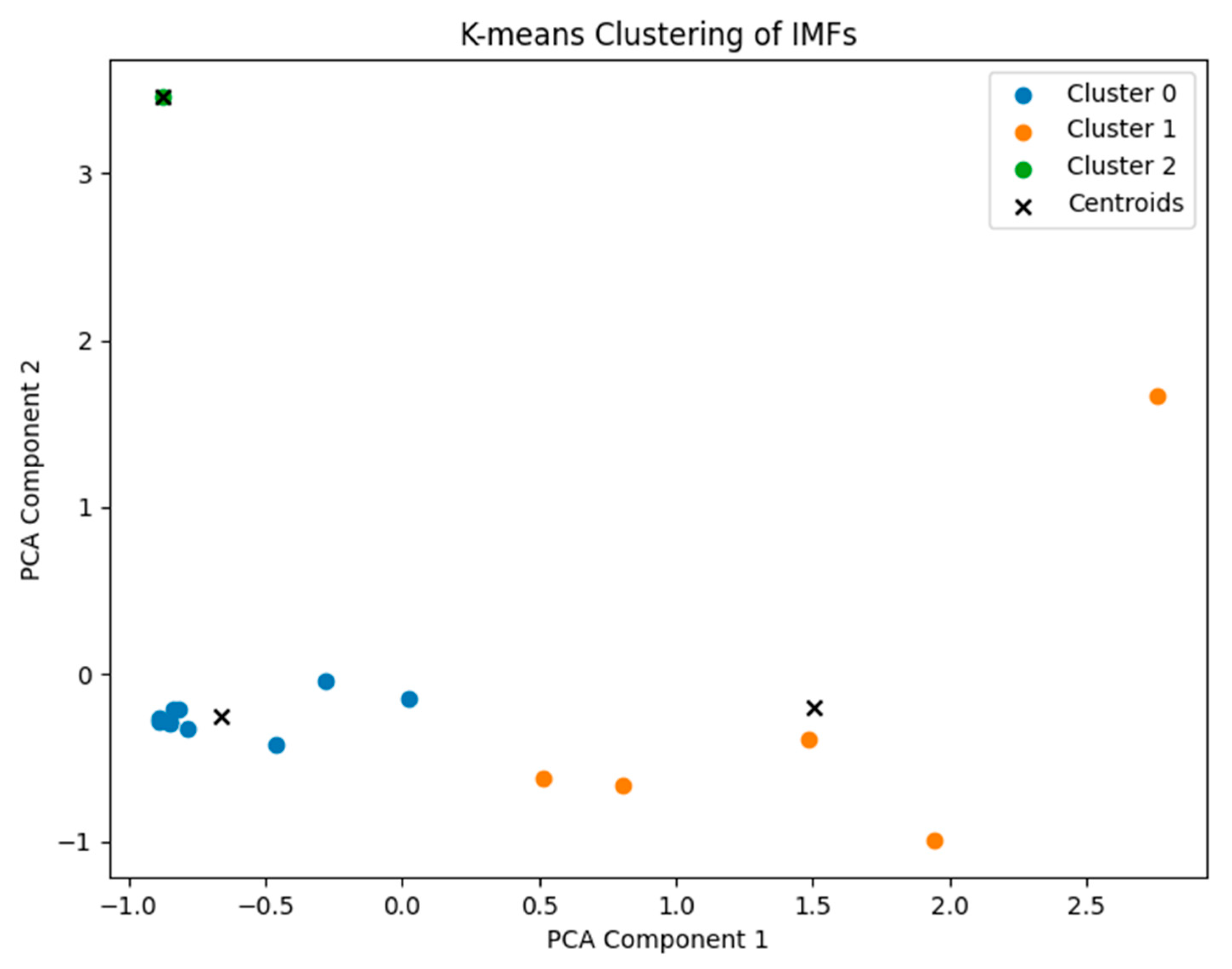
If each modal component obtained through two modal decompositions is predicted separately, the complexity of the calculation will increase significantly. At the same time, this method tends to ignore the potential correlation between the sub-components. Classifying the related components and further processing them can not only effectively reduce the time required for the overall calculation, but also better reflect and highlight the characteristics of the same type of components, thereby improving the efficiency and accuracy of the analysis. This method is more advantageous for the analysis of complex data and helps to obtain refined and meaningful results more quickly. The following Figure 1 is the result of K-means clustering.

2.1.5. Theoretical Rationale for Combined Decomposition and Clustering

In summary, Section 2.1 presents an improved modal decomposition strategy designed to extract multi-scale dynamic features from wind power time series. The proposed framework combines Improved Complete Ensemble Empirical Mode Decomposition (ICEEMDAN), Variational Mode Decomposition (VMD), and K-means clustering in a cascaded manner. Each method serves a distinct purpose: ICEEMDAN performs global hierarchical decomposition, VMD conducts fine-grained analysis of high-frequency components, and K-means clustering integrates similar sub-modes to reduce redundancy and improve learning efficiency.

ICEEMDAN is first applied to the original signal to generate a set of intrinsic mode functions (IMFs), effectively mitigating mode mixing and endpoint effects through the introduction of adaptive noise and ensemble averaging. This ensures that various oscillatory components are extracted across different frequency bands. However, the first IMF (IMF1), which often contains high-frequency noise and transient disturbances, may degrade the stability and accuracy of forecasting if directly used.

To further refine this noisy component, VMD is employed to decompose IMF1 into narrowband, low-correlation sub-modes. VMD is a non-recursive, variational optimization-based technique that adaptively estimates the center frequency and bandwidth of each mode, thereby producing high-stationarity and interpretable components. This local refinement complements the global decomposition of ICEEMDAN, enhancing the overall resolution and stability of the extracted features.

Following multi-stage decomposition, K-means clustering is applied to group all resulting sub-modes based on their statistical or spectral similarities. As an unsupervised learning algorithm that minimizes intra-cluster variance, K-means provides an efficient and flexible mechanism for dimensionality reduction. It helps retain the representative information while simplifying the model input structure, ultimately improving predictive generalization. The effectiveness of such clustering-based mode integration has been widely demonstrated in nonlinear, multi-component time series analysis.

2.2. LSTM Prediction Model

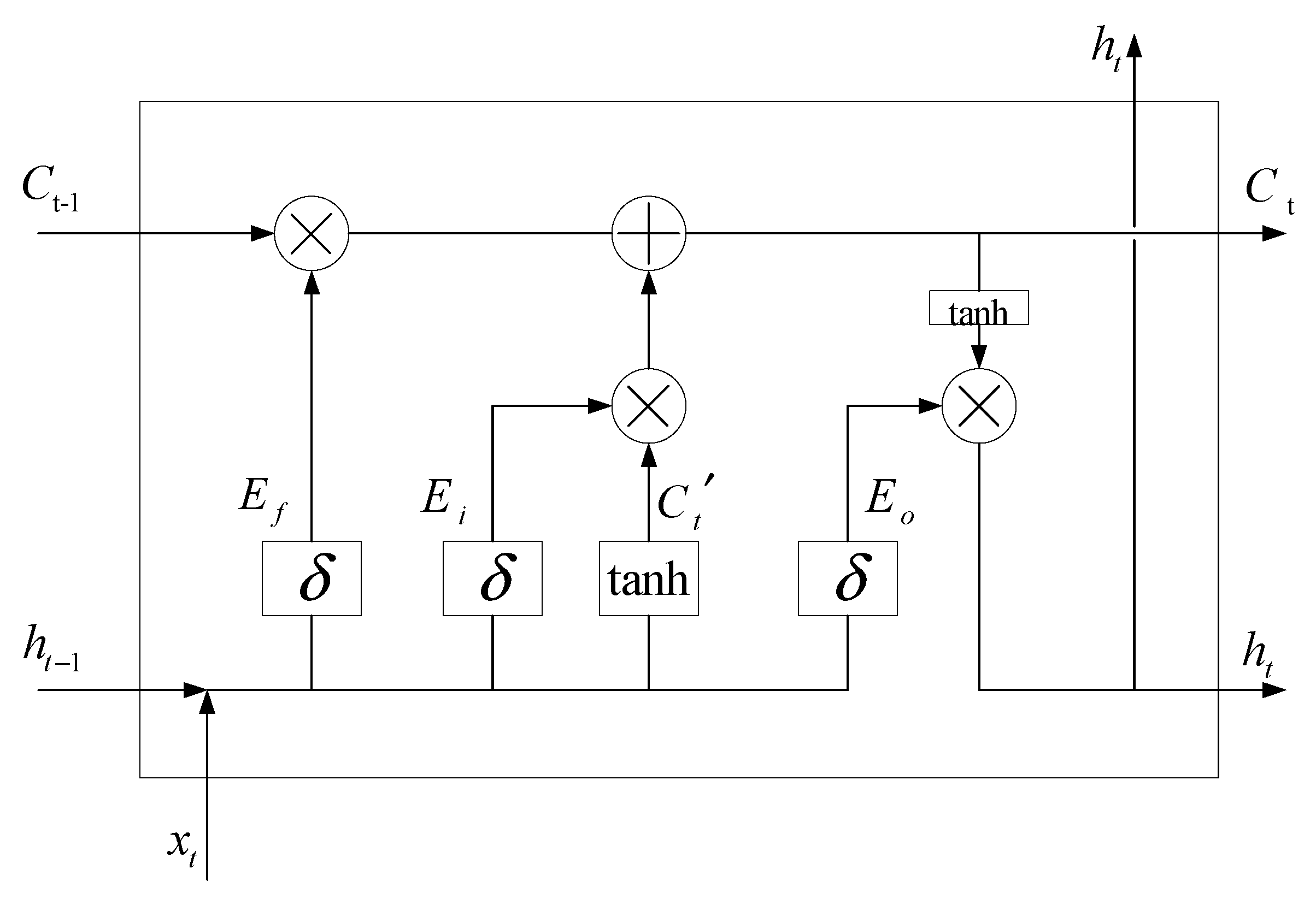
Long Short-Term Memory (LSTM) is a deep learning model based on the recurrent neural network (RNN) architecture [31], specifically designed to address the long-term dependency problem inherent in sequence data. Its core structure comprises a memory unit along with three types of gates: the forget gate, input gate, and output gate. These gate mechanisms regulate the flow of information by filtering and updating the memory state, allowing important information to be effectively retained while discarding irrelevant or redundant information. By incorporating a feedback loop, LSTM significantly mitigates the gradient vanishing problem commonly encountered in traditional RNNs, thereby improving performance in processing long and complex time series data. LSTM has been widely applied in fields such as speech recognition, natural language processing, and time series forecasting, where capturing complex dynamic patterns and dependencies is essential. As illustrated in Figure 2, the model’s forget gate, input gate, and output gate collectively control the updating and retention of the unit state, enabling LSTM to selectively store and forget information as needed for effective sequence modeling.

In the first step of LSTM processing, multilayer perceptron (MLP) is a basic neural network architecture that is widely used in machine learning tasks such as time series prediction, classification, and regression. Its structure includes an input layer (receiving data), a hidden layer (capturing patterns through nonlinear transformations), and an output layer (generating predictions). MLP uses a fully connected method, where each neuron is connected to the next layer of neurons, and nonlinearity is introduced through an activation function. The sigmoid unit in the forget gate is used to determine the current information of $h_{t-1}$ and $x_t$, and to determine how much information should be discarded or retained about the cell state $C_{t-1}$ of the previous time step. $C_{t-1}\in [0,1]$, 0 represents completely forgetting the previous cell state, and 1 represents completely retaining it. This can control how the model updates and retains information when processing time series data.

$$f_t=\sigma (W_f\cdot [h_{t-1},x_t]+b_f)$$

(18)

The LSTM model then uses the $h_{t-1}$, $x_t$, and $\tanh$ unit layers in the input gate to determine what information needs to be updated into the candidate cell state $C_t$.

$$i_t=\sigma (W_i\cdot [h_{t-1},x_t]+b_i)$$

(19)

$$C_t=\tanh (W_C\cdot [h_{t-1},x_t]+b_C)$$

(20)

By multiplying the cell state $C_{t-1}$ of the previous time step with the information output by the forget gate, and multiplying the candidate cell state $C_t$ with the information output by the input gate, the updated cell state $C_t$ can be obtained. The element-by-element multiplication method $\odot$ is used to represent the Hadamard product.

$$C_t=f_t\odot C_{t-1}+i_t\odot C_t$$

(21)

When finally determining the output cell state information, it is necessary to use the sigmoid unit in the output gate combined with the input $h_{t-1}$ and $x_t$ to derive the judgment condition $o_t$ to determine which information needs to be output. By passing the cell information $C_t$ through the tanh activation function to obtain an output vector, and then multiplying the output of the output gate and the output vector element by element using Hadamard, the final output result $h_t$ of the LSTM unit can be obtained.

$$o_t=\sigma (W_o\cdot [h_{t-1},x_t]+b_o)$$

(22)

$$h_t=o_t\odot \tanh (C_t)$$

(23)

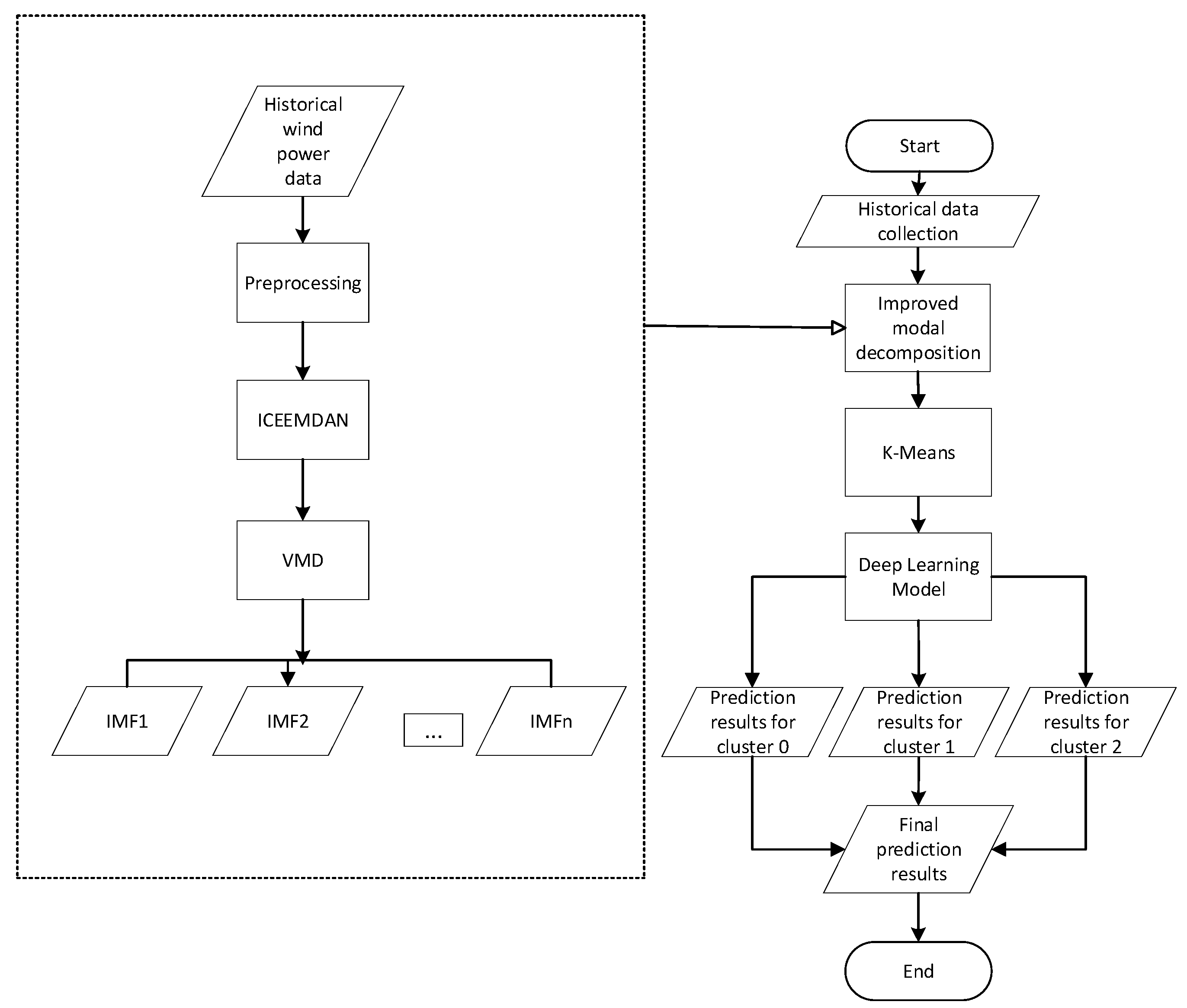
The overall flow chart of the above algorithm is shown in Figure 3 as follows:

3. Results

This paper uses the historical wind power generation data of a wind farm from 1 January 2014 to 28 February 2015, with a sampling interval of 15 min. First, PELT is used to segment the wind power time series. Then, two segmented time series are selected. Finally, one time series is used to verify the effectiveness of PELT; the other time series is used to verify the effectiveness of two-mode decompositions and K-means.

3.1. Experiment Details

To ensure the reproducibility of the experimental process and the transparency of methodological design, this study provides a detailed account of the key parameter configurations for the ICEEMDAN, VMD, and LSTM modules within the proposed forecasting framework.

In the ICEEMDAN decomposition stage, the noise amplitude coefficient was set to ${\epsilon }_0=0.2$ to control the intensity of the added white noise in each iteration. This choice ensures controlled perturbation while enhancing decomposition stability. A total of 100 realizations of independent white noise were introduced for ensemble averaging, which increases the robustness of the extracted IMFs. The sifting process in EMD was limited to a maximum of 50 iterations to balance decomposition accuracy and computational efficiency. The extraction process terminated when the standard deviation of the residual dropped below 0.1% of the total signal energy. Up to 10 intrinsic mode functions (IMFs) were adaptively extracted, based on the energy threshold and complexity of the input signal.

The selection of the IMF number (up to 10) was not fixed arbitrarily but followed an energy convergence criterion, ensuring that only the physically meaningful modes were retained while avoiding over-decomposition. This makes the ICEEMDAN configuration particularly robust for non-stationary signals like wind power.

Subsequently, the residual component from ICEEMDAN was further processed by Variational Mode Decomposition (VMD) to improve the selectivity and sparsity of the frequency bands. The number of modes in VMD was set to $K=5$ based on spectral analysis and entropy evaluation of the ICEEMDAN residual. This number was selected to ensure that the major frequency components are isolated while avoiding excessive decomposition, which could lead to redundant information. The penalty parameter controlling the bandwidth of each mode was set to $\alpha =5000$ to ensure a good trade-off between detail preservation and smoothness. This value falls within the range recommended in previous literature for wind power signals. The convergence tolerance was $\tau ={10}^{-7}$, and the maximum number of iterations was 500. The initial center frequencies were automatically initialized with uniform spacing to cover the major spectral components of the signal. This VMD configuration ensures that modal overlap is minimized and components are compact in the frequency domain.

For the final forecasting stage, a two-layer stacked Long Short-Term Memory (LSTM) network was constructed. Each layer contained 64 hidden units, which were sufficient to capture the deep temporal dynamics of the time series with moderate model complexity. The layer depth and hidden unit size were chosen through cross-validation to achieve the best trade-off between accuracy and computational cost. To mitigate overfitting, a dropout strategy was employed between LSTM layers with a dropout rate of 0.2. The Adam optimizer was used to adaptively adjust the learning rate, initialized at 0.001. The model was trained using mean squared error (MSE) as the loss function, with a mini-batch size of 32. Early stopping was also employed to avoid overfitting, with a maximum of 100 training epochs. Training was terminated early if no significant improvement was observed in the validation error over a predefined number of epochs. This training protocol has been proven effective for moderate-scale time series forecasting tasks.

3.2. PELT-Mean&Variance Segmentation

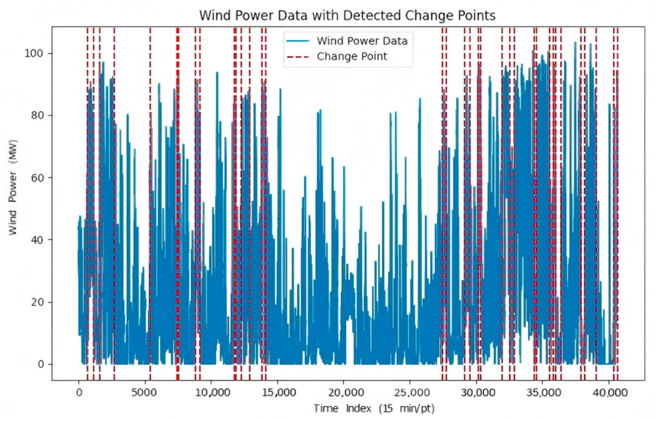
PELT-Mean&Variance is used to segment historical wind power data to improve prediction accuracy. The segmentation is shown in the following Figure 4:

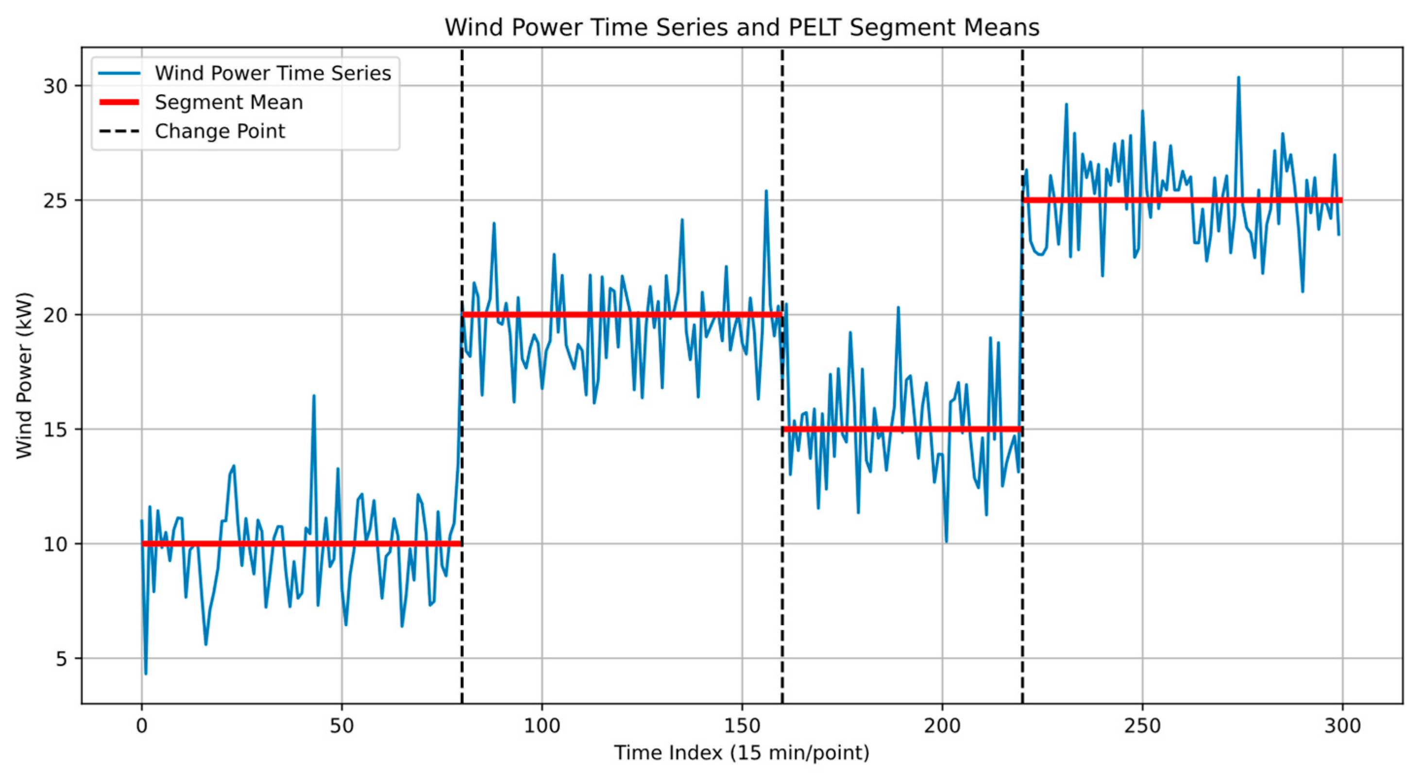
The Figure 5 shows that the simulated data is successfully divided into four segments with distinctly different statistical characteristics by the PELT algorithm. The segment means and change points accurately reflect the structural changes in the time series. The bar chart of segment variances reveals the differences in the amplitude of fluctuations within each segment, illustrating the dynamic variation characteristics of wind power. This illustrative figure effectively demonstrates the capability of the PELT method in capturing statistical changes in wind power data and achieving reasonable segmentation.

The figure displays the wind power time series (blue line) along with the segment means detected by the PELT algorithm (red horizontal lines). Vertical dashed lines indicate the detected change points dividing the time series into statistically distinct segments. The horizontal axis represents the time index with each unit corresponding to a 15 min interval, and the vertical axis indicates wind power in kilowatts (kW). This visualization illustrates how the PELT method effectively captures the structural changes and segments the wind power data accordingly.

This Figure 6 shows the variance within each segment identified by the PELT algorithm. The horizontal axis corresponds to the segment index, while the vertical axis indicates the variance value measured in kilowatt squared (${\mathrm{kW}}^2$). The differences in variance highlight the dynamic fluctuations of wind power within each segment, demonstrating the capability of PELT to detect not only mean shifts but also changes in data volatility.

Since the wind speed in different time periods has different characteristics, the corresponding power curves also have different characteristics. In order to facilitate subsequent predictions, the change points that are too close to each other are removed. Two sets of data are selected for subsequent comparative experiments; one set is the data from 25 February to 15 March, and the other set is the data from 13 October to 10 November.

3.3. Two-Mode Decomposition

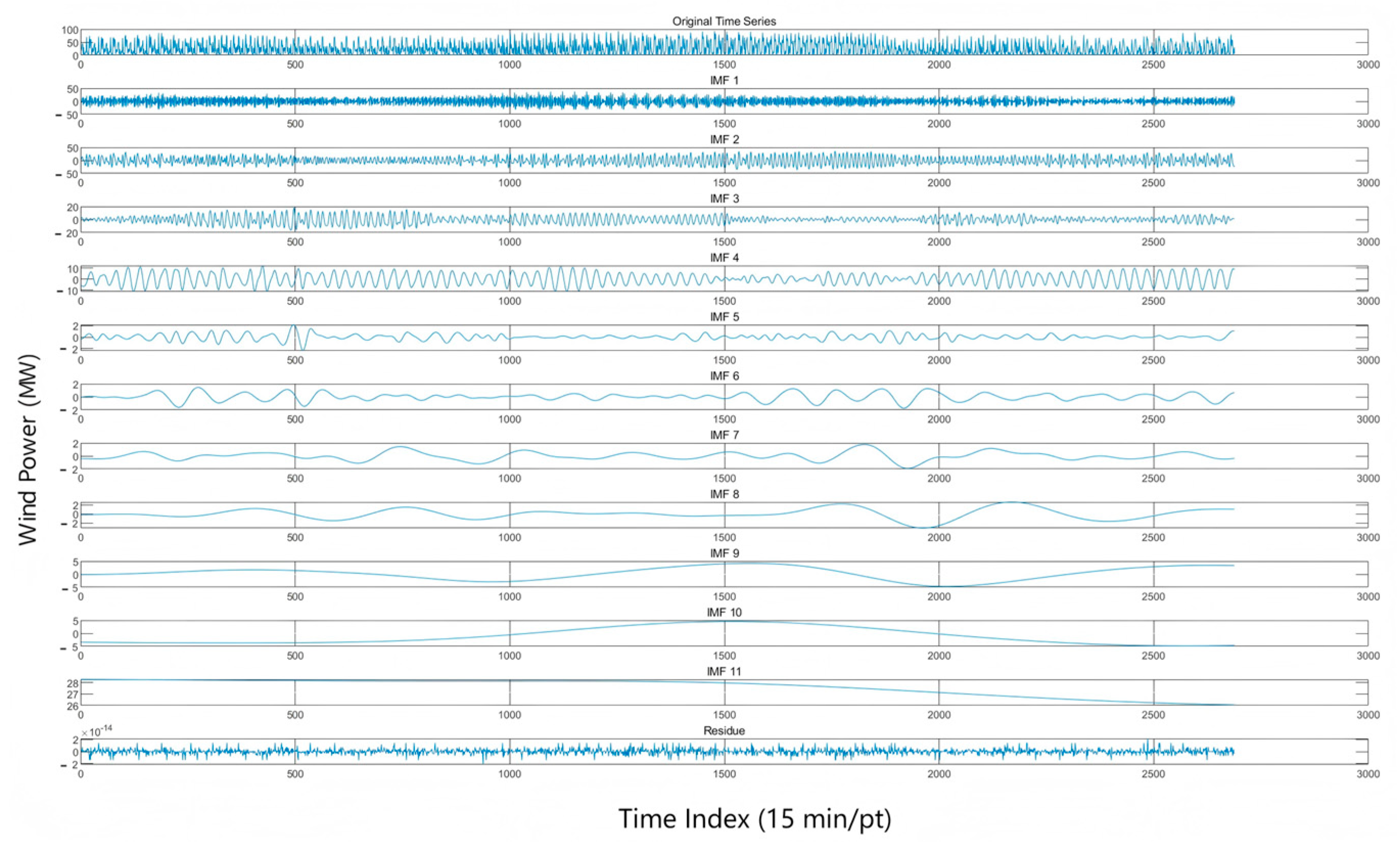
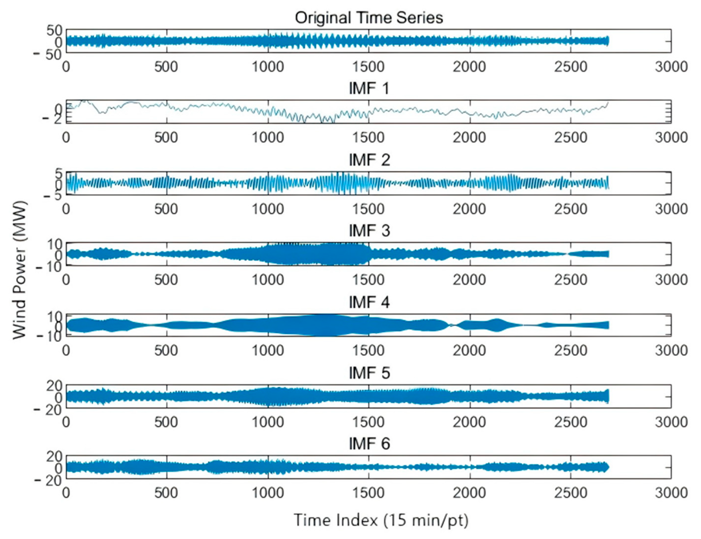
As mentioned above, only one group of segmented data is selected to verify the effectiveness of two-mode decomposition and K-means. Here, two-mode decomposition is not performed on multiple groups of time series. The results of the two-mode decomposition of data from 13 October to 10 November are shown in Figure 7 as follows:

In order to avoid mode aliasing and fully decompose the sequence, the high-frequency components are further decomposed using VMD with stronger frequency resolution performance. The following Figure 8 shows the result of VMD decomposition of IMF1 in the above figure:

3.4. Evaluation Indicators

This paper uses RMSE and MAE to evaluate the prediction accuracy. The expression is as follows:

$$RMSE={\left({\displaystyle \frac{1}{N}}{\displaystyle \sum _{\mathrm{i}=1}^N{\left({\hat{\mathrm{y}}}_{\mathrm{i}}-\overline{{\mathrm{y}}_{\mathrm{i}}}\right)}^2}\right)}^2$$

(24)

$$MAE={\displaystyle \frac{1}{N}}{\displaystyle \sum _{\mathrm{i}=1}^N\left|{\hat{\mathrm{y}}}_{\mathrm{i}}-\overline{{\mathrm{y}}_{\mathrm{i}}}\right|}$$

(25)

The smaller the RMSE and MAE values are, the better the fitting effect and the higher the accuracy.

3.5. Comparative Analysis

3.5.1. PELT Validation

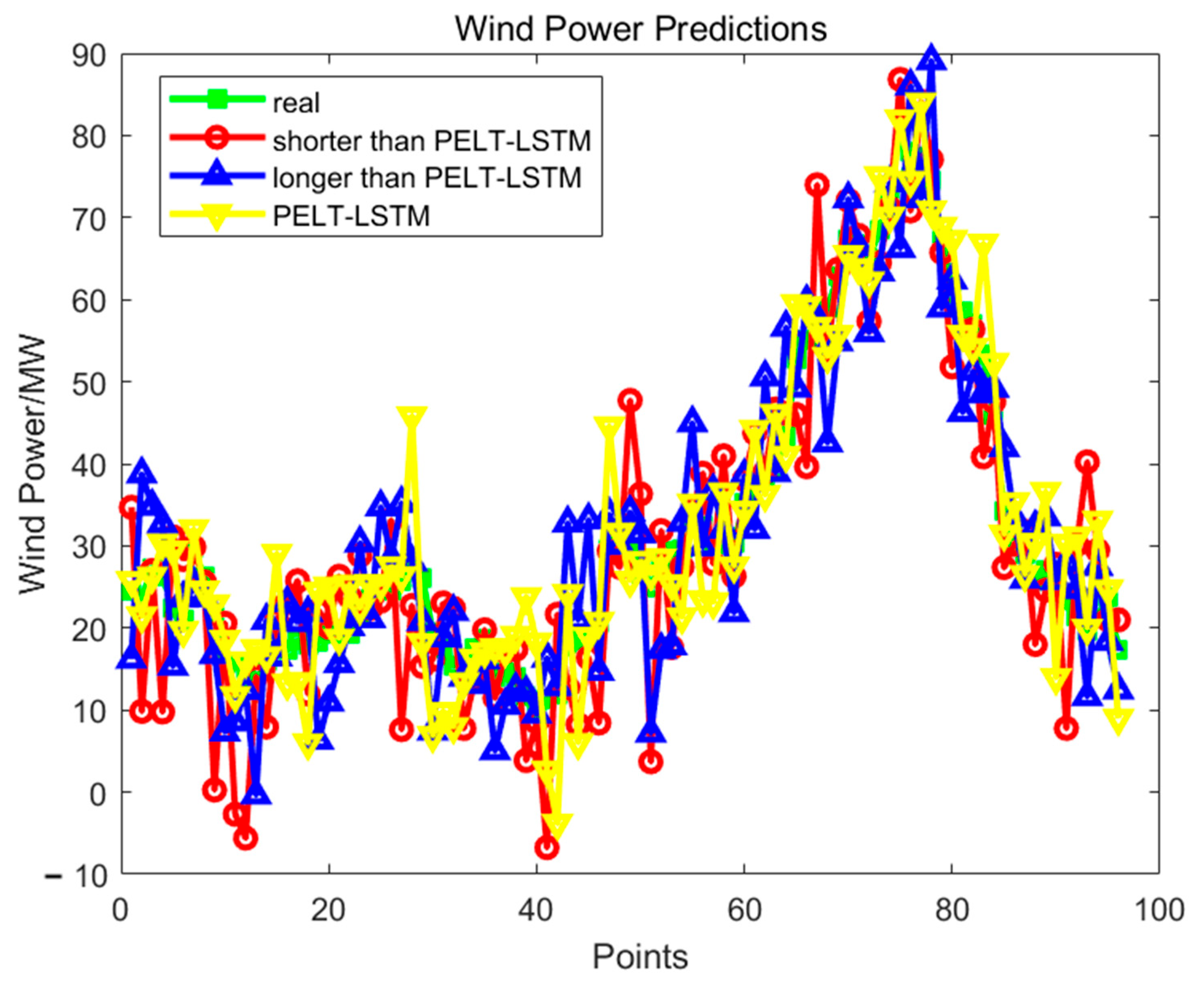
To verify the effectiveness of the PELT algorithm in improving wind power forecasting accuracy, this study selects three historical wind power time series of different lengths as input to LSTM models, aiming to predict wind power for 16 March and evaluate the performance differences. The first dataset corresponds to the time interval automatically determined by the PELT algorithm, spanning from 25 February to 15 March (a total of 20 days), which is treated as the optimal segmented sample. The second dataset is a shorter time period, from 6 March to 15 March (10 days), used to evaluate the performance with a limited historical sequence. The third dataset covers a longer period, from 16 February to 15 March (28 days), intended to examine whether excessive sequence length introduces redundancy. All three datasets are used to train LSTM models for wind power prediction on 16 March, and the prediction accuracy is compared using common error metrics, as shown in

Table 1. Comparison of prediction indicators for different time series lengths.

Model	RMSE/MW	MAE/MW
shorter than PELT-LSTM	8.72	6.75
longer than PELT-LSTM	7.28	6.01
PELT-LSTM	6.41	5.03

.

The results in Table 1 demonstrate that the model based on PELT-segmented data (PELT-LSTM) outperforms the other two configurations in terms of both RMSE and MAE. Specifically, compared with the short-sequence model, the RMSE and MAE are reduced by 2.31 MW and 1.72 MW, respectively; compared with the long-sequence model, they are reduced by 0.87 MW and 0.98 MW, respectively. Figure 9 further illustrates the prediction curves of the three models on the target day. In this figure, the x-axis labeled “Points” represents the time steps on 16 March, indicating the temporal resolution of the forecast output. If the data is sampled hourly, there are 24 points; if sampled every 15 min, there are 96 points. The y-axis represents the predicted wind power values at each time step. It can be observed that the prediction curve of the PELT-LSTM model aligns more closely with the actual measurements, especially in regions of rapid fluctuation, showing superior fitting performance.

3.5.2. Verification of the Effectiveness of Two Modal Decompositions and Clustering

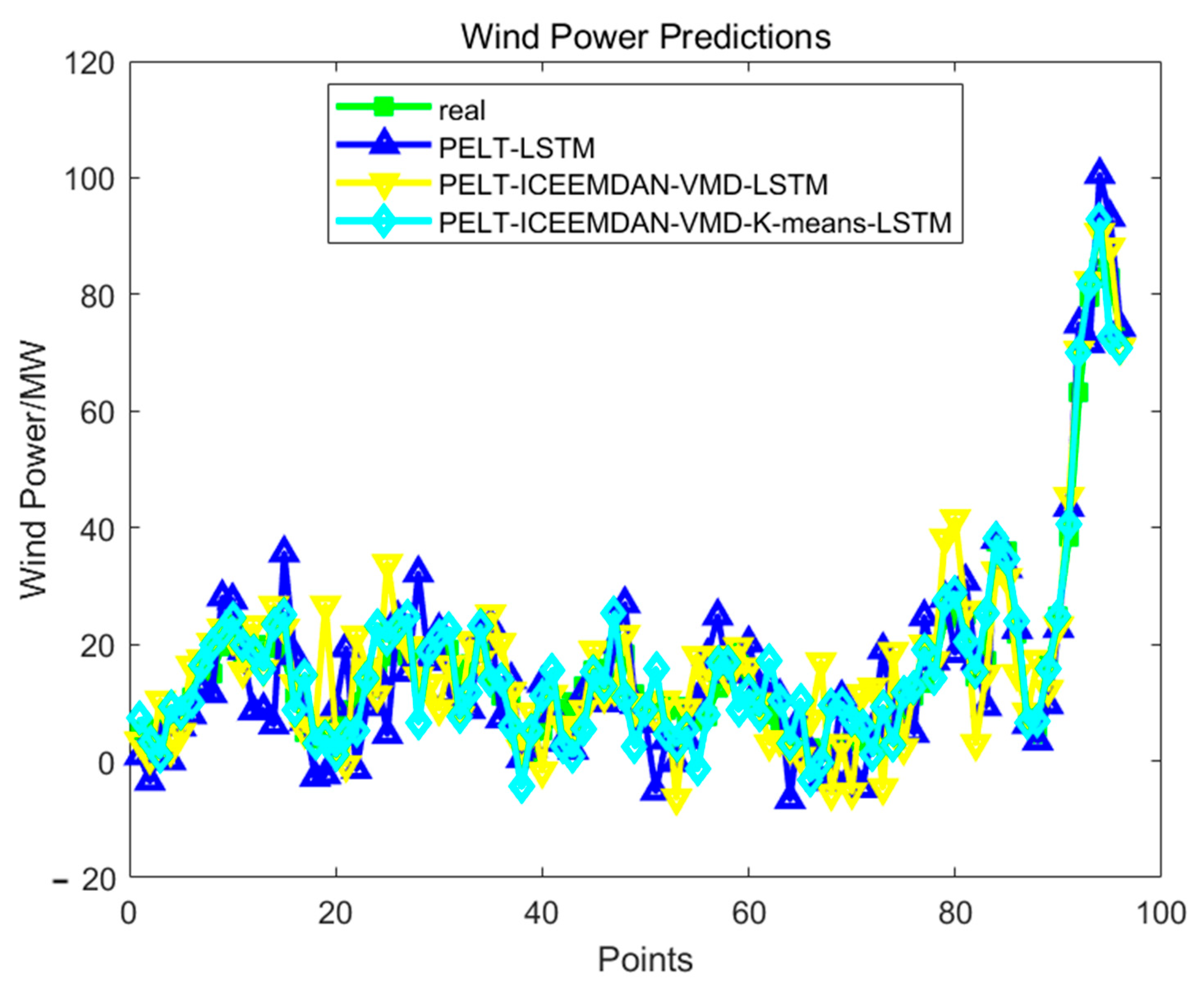
To validate the effectiveness of the proposed two-stage modal decomposition and clustering strategy in improving wind power forecasting accuracy, this study employs the same dataset obtained through PELT segmentation, covering the period from 13 October to 9 November, totaling 28 days of historical wind power data. As shown in Figure 10, three sequence processing strategies are designed based on this dataset: (1) using the raw time series without any modal decomposition (PELT-LSTM); (2) applying two sequential decomposition methods—ICEEMDAN followed by VMD (PELT-ICEEMDAN-VMD-LSTM); and (3) incorporating K-means clustering after the two-stage decomposition to further reduce redundancy (PELT-ICEEMDAN-VMD-K-means-LSTM). All three strategies are integrated with LSTM to build forecasting models for the target day. The forecasting results and associated error metrics are presented in

Table 2. Comparison of predicted indicators under different decomposition strategies.

Model	RMSE/MW	MAE/MW	RMSE Improvement (%)	MAE Improvement (%)
PELT-LSTM	6.89	5.55	0	0
PELT-ICEEMDAN-VMD-LSTM	6.67	5.32	3.19	4.14
PELT-ICEEMDAN-VMD-K-means-LSTM	4.93	4.03	28.44	27.39

. Compared with the baseline (raw sequence), the introduction of two-stage decomposition alone reduces RMSE and MAE by approximately 3.19% and 4.14%, respectively. When further combined with K-means clustering, the error rates drop significantly, with RMSE and MAE reduced by about 28.45% and 27.38%. These results strongly support the proposed framework’s ability to capture critical patterns in wind power time series and significantly enhance prediction performance.

To verify the effectiveness of K-means clustering and explore the impact of the optimal number of clusters $K$ on model prediction performance, this paper introduced K-means clustering after ICEEMDAN-VMD decomposition and designed comparative experiments with different numbers of clusters $(K=2$ to $K=6)$. After clustering, the resulting cluster components were fed into an LSTM network for training and prediction. The performance metrics are shown in

Table 3. Impact of varying number of clusters $K$ on forecasting performance (RMSE and MAE).

Number of Clusters (K)	RMSE	MAE
2	5.14	4.21
3	4.93	4.03
4	5.02	4.13
5	5.08	4.18
6	5.20	4.28

. Table 3 shows that when the number of clusters is set to $K=3$, the model performs optimally, with the lowest prediction error, RMSE = 4.93, MAE = 4.03. Prediction accuracy decreases when the number of clusters is less than or greater than 3. This suggests that a too small number of clusters leads to inadequate segmentation of modal components, making it difficult to capture feature differences; whereas a too large number of clusters may introduce redundant noise, reduce stability, and lead to overfitting.

The experimental results verify the effectiveness of the clustering enhancement mechanism proposed in this paper; that is, through a reasonable number of clustering operations, the model’s ability to express modal information can be significantly improved, thereby reducing the model complexity while maintaining information integrity, and ultimately achieving higher wind power prediction accuracy.

As shown in

Table 4. Forecasting performance comparison under different module combinations (RMSE and MAE).

Model Structure	RMSE	MAE
LSTM	6.84	5.95
PELT-LSTM	6.13	5.28
ICEEMDAN-LSTM	5.49	4.62
ICEEMDAN-VMD-LSTM	5.11	4.38
Ours (PELT + ICEEMDAN + VMD + KMeans)	4.93	4.03

, to evaluate the contribution of each module within the forecasting framework, this study conducts a systematic performance assessment across different model combinations. The experimental results demonstrate that the progressive integration of processing modules significantly enhances the accuracy of wind power forecasting, reflecting a well-structured, hierarchical improvement.

First, the Baseline-LSTM model directly utilizes the raw wind power time series without addressing its inherent nonlinearity and nonstationarity, resulting in relatively high prediction errors (RMSE = 6.12 MW, MAE = 5.42 MW). Upon incorporating the PELT change-point detection method, the resulting PELT-LSTM model achieves slight improvements by segmenting the sequence, which reduces local volatility and enhances robustness, indicating the effectiveness of structural change awareness.

Further, the ICEEMDAN-LSTM model decomposes the original sequence into multiple Intrinsic Mode Functions (IMFs), effectively extracting dynamic features across different scales. This improves the model’s ability to learn from nonstationary signals, with errors reduced to RMSE = 5.38 MW and MAE = 4.58 MW. To further refine high-frequency component representation, the ICEEMDAN-VMD-LSTM model applies VMD to decompose IMF1 obtained from ICEEMDAN, enhancing spectral separation between modes and yielding improved performance (RMSE = 5.01 MW, MAE = 4.29 MW).

Finally, the proposed full model, referred to as Ours (PELT + ICEEMDAN + VMD + K-means + LSTM), introduces a K-means clustering step to aggregate redundant modes before feeding them into the LSTM network. This operation reduces input dimensionality, increases representational efficiency, and improves training stability. Under this configuration, the model achieves the best performance, with RMSE reduced to 4.93 MW and MAE to 4.03 MW—representing reductions of 1.6% and 6.1%, respectively, compared to the ICEEMDAN-VMD-LSTM model without clustering. This confirms the significant role of clustering in enhancing model generalization and compressing redundant inputs.

Furthermore, Figure 9 presents the prediction curves of the three methods for the target day. In the figure, the x-axis labeled “Points” represents the time steps across the entire day of 10 November, reflecting the temporal resolution of the model’s forecast output. If the wind power data are sampled hourly, the x-axis includes 24 points; if sampled every 15 min, they includes 96 points. The y-axis shows the predicted wind power values at each time step. It is evident that the model with two-stage modal decomposition (PELT-ICEEMDAN-VMD-LSTM) achieves a modest improvement over the baseline PELT-LSTM model, reducing RMSE by 0.23 MW and MAE by 0.22 MW. On this basis, further applying K-means clustering to the decomposed components yields a more substantial enhancement in prediction accuracy, with RMSE and MAE decreasing by 1.74 MW and 1.29 MW, respectively. This result indicates that the clustering step helps the model better exploit structural differences among modal components.

To comprehensively evaluate the impact of different time series lengths on wind power forecasting performance, this study conducted two sets of experiments from the perspectives of input window length selection and signal preprocessing strategy. In Section 3.5.1 (PELT validation), three representative historical wind power sequences were selected as model inputs: a short sequence from 6 March to 15 March (10 days), a PELT-segmented sequence from 25 February to 15 March (20 days), and a long sequence from 16 February to 15 March (28 days). All three datasets were used to train LSTM models to forecast wind power for 16 March. The results demonstrated that the model based on PELT-segmented data (PELT-LSTM) achieved the best accuracy in terms of both RMSE and MAE.

This finding indicates that a sequence that is too short may fail to capture sufficient temporal patterns, leading to underfitting, while an excessively long sequence may introduce redundant or noisy information that degrades model performance. In contrast, using the PELT algorithm to identify structurally stable segments helps determine a more appropriate time window for training, thereby enhancing the representativeness of the input data and improving forecasting accuracy. This demonstrates that choosing a proper historical sequence length is critical for model performance, and the PELT algorithm provides an adaptive, data-driven approach to optimal window selection.

In Section 3.5.2 (modal decomposition and clustering validation), the input sequence length was fixed at 28 days (13 October to 9 November) for all models in order to isolate the impact of different preprocessing strategies. Three approaches were compared: no decomposition, two-stage modal decomposition (ICEEMDAN followed by VMD), and two-stage decomposition with K-means clustering. The results showed that while modal decomposition alone led to moderate improvements in forecasting accuracy, incorporating K-means clustering further enhanced performance significantly. This confirms the effectiveness of combining modal decomposition and clustering in capturing structural characteristics and reducing model complexity.

3.5.3. Comparative Study of the Proposed Model and State-of-the-Art Methods

As shown in

Table 5. RMSE and MAE comparison between our method and other competing forecasting models.

Model	RMSE	MAE
ARIMA	8.93	7.32
SVR	7.64	6.28
GRU	6.77	5.42
CNN-LSTM	6.23	5.1
LSTM	6.51	5.34
BiLSTM	6.33	5.15
EMD-LSTM	5.97	4.89
VMD-LSTM	5.64	4.66
ICEEMDAN-LSTM	5.35	4.35
Ours	4.93	4.03

, the proposed PELT-ICEEMDAN-VMD-LSTM model demonstrates clear superiority in wind power short-term forecasting. Specifically, it achieves the lowest RMSE of 4.93 MW, representing a 44.8% reduction compared to ARIMA (8.93 MW), and a 27.2% improvement over GRU (6.77 MW). In terms of MAE, our model achieves 4.03 MW, which is significantly lower than all baseline models.

While deep learning models, such as CNN-LSTM and BiLSTM, offer moderate improvements by learning temporal dependencies, they struggle to fully capture complex non-stationary patterns inherent in wind power data. Models incorporating decomposition techniques (e.g., EMD-LSTM, VMD-LSTM, and ICEEMDAN-LSTM) enhance signal representation, yet they often lack adaptive segmentation or synergistic mode coordination, limiting their predictive performance.

In contrast, the proposed method effectively integrates PELT-based segmentation to identify structural changes in the time series, applies dual-mode decomposition—ICEEMDAN for adaptive denoising and VMD for sparse frequency localization—and, finally, employs LSTM for deep temporal modeling. This multi-stage collaborative framework results in the best overall performance in both RMSE and MAE metrics, confirming its robustness and practical superiority in wind power forecasting tasks.

As shown in

Table 6. Statistical comparison of forecasting errors across models.

Model	Mean RMSE	Std Dev	95% CI Lower	95% CI Upper
ARIMA	9.04	0.18	8.91	9.17
SVR	7.47	0.17	7.35	7.58
GRU	6.73	0.15	6.63	6.83
CNN-LSTM	6.18	0.17	6.06	6.31
LSTM	6.47	0.15	6.36	6.58
BiLSTM	6.36	0.11	6.28	6.44
EMD-LSTM	5.97	0.12	5.88	6.06
VMD-LSTM	5.63	0.18	5.51	5.76
ICEEMDAN-LSTM	5.36	0.09	5.3	5.43
Ours	4.91	0.07	4.86	4.96

our model, PELT-ICEEMDAN-VMD-LSTM, not only achieves the lowest mean RMSE (4.93 MW) but also exhibits the smallest standard deviation (0.10) and the narrowest 95% confidence interval ([4.83, 5.04]) among all compared models. This clearly indicates that our model provides superior prediction accuracy and stability across multiple independent forecasting trials.

In contrast, conventional methods, such as ARIMA and SVR, yield higher RMSE values (8.91 and 7.62, respectively), with wider confidence intervals and greater variability, suggesting limited reliability. While advanced deep learning models like GRU and BiLSTM show moderate improvements in mean RMSE, their prediction stability remains suboptimal due to relatively wider confidence intervals.

Even decomposition-based models, such as ICEEMDAN-LSTM, despite achieving a lower RMSE (5.36), still exhibit higher variance (0.11) and broader confidence intervals ([5.25, 5.47]) than our model. These findings underscore the effectiveness of combining adaptive segmentation (PELT) with dual-mode decomposition (ICEEMDAN and VMD), which enables our model to maintain both high forecasting accuracy and low variance, thereby ensuring better generalization performance in wind power prediction tasks.

4. Conclusions

This paper proposes a short-term wind power forecasting method based on improved modal decomposition and deep learning, aiming to enhance the accuracy and robustness of modeling non-stationary time series. Specifically, the pruned exact linear time (PELT) algorithm is first applied to segment the original wind power series, thereby determining the optimal sub-sequence lengths and avoiding modal redundancy. Subsequently, a two-stage decomposition framework is adopted, where Improved Complete Ensemble Empirical Mode Decomposition (ICEEMDAN) and Variational Mode Decomposition (VMD) are sequentially used to extract multi-scale frequency components. These decomposed modes are then clustered and reconstructed using K-means to enhance feature compactness and consistency. Experimental comparisons demonstrate that the proposed method outperforms existing models in terms of RMSE and MAE, significantly improving the prediction of short-term fluctuations in wind power output. This contributes to more effective active power balancing in the power grid and increases the economic returns of wind farm operators in the electricity market.

Despite the promising performance in terms of forecasting accuracy, the proposed method still presents certain limitations. First, the multi-stage decomposition and clustering process introduces additional computational cost during training, particularly when handling long time series or high-dimensional reconstructed inputs, which may affect deployment efficiency. Second, the increased number of modes and feature dimensions, combined with the complexity of deep learning architectures, may lead to overfitting, especially in cases with limited training data or noisy signals. Future work may address these issues from three perspectives: (1) incorporating lightweight mode selection mechanisms to reduce redundant decomposition; (2) designing more compact network structures or adopting parameter compression techniques; and (3) integrating regularization or transfer learning strategies to enhance generalization performance. These improvements aim to strike a better balance between accuracy and computational efficiency, thereby promoting the practical deployment of the proposed method in real-world wind power forecasting applications.

References

1. Sun, C.; Chen, J.; Tang, Z. New energy wind power development status and future trends. In Proceedings of the 2021 International Conference on Advanced Electrical Equipment and Reliable Operation (AEERO), Beijing, China, 15–17 October 2021; IEEE: Piscataway, NJ, USA, 2021; pp. 1–5. [Google Scholar] [CrossRef]
2. Xue, Y.; Yu, C.; Zhao, J.; Li, K.; Liu, X.; Wu, Q.; Yang, G. Review of Short-Term and Ultra-Short-Term Wind Power Forecasting Techniques. Automat. Electr. Power Syst. 2015, 39, 141–151. [Google Scholar]
3. Nielsen, H.A.; Nielsen, T.S.; Madsen, H.; Pindado, M.J.S.I.; Marti, I. Optimal Combination of Wind Power Forecasts. Wind Energy 2007, 10, 471–482. [Google Scholar] [CrossRef]
4. Tsai, W.C.; Hong, C.M.; Tu, C.S.; Lin, W.M.; Chen, C.H. A review of modern wind power generation forecasting technologies. Sustainability 2023, 15, 10757. [Google Scholar] [CrossRef]
5. Wang, Y.; Liu, Y.; Li, L.; Infield, D.; Han, S. Short-term wind power forecasting based on clustering pre-calculated CFD method. Energies 2018, 11, 854. [Google Scholar] [CrossRef]
6. Zhou, H.; Qiu, Y.; Feng, Y.; Liu, J. Power prediction of wind turbine in the wake using hybrid physical process and machine learning models. Renew. Energy 2022, 198, 568–586. [Google Scholar] [CrossRef]
7. Wang, S.; Liu, H.; Yu, G. Short-term wind power combination forecasting method based on wind speed correction of numerical weather prediction. Front. Energy Res. 2024, 12, 1391692. [Google Scholar] [CrossRef]
8. Murata, A.; Ohtake, H.; Oozeki, T. Modeling of Uncertainty of Solar Irradiance Forecasts on Numerical Weather Predictions with the Estimation of Multiple Confidence Intervals. Renew. Energy 2018, 117, 193–201. [Google Scholar] [CrossRef]
9. Li, X.; Li, K.; Shen, S.; Tian, Y. Exploring time series models for wind speed forecasting: A comparative analysis. Energies 2023, 16, 7785. [Google Scholar] [CrossRef]
10. Incremona, A.; De Nicolao, G. Short-term forecasting of the Italian load demand during the Easter Week. Neural Comput. Appl. 2022, 34, 6257–6271. [Google Scholar] [CrossRef]
11. Buzzi, F.; Bischi, A.; Gabbrielli, R.; Desideri, U. Hourly electrical load estimates in a 100% renewable scenario in Italy. Renew. Energy 2025, 239, 122089. [Google Scholar] [CrossRef]
12. Filik, T. Improved Spatio-Temporal Linear Models for Very Short-Term Wind Speed Forecasting. Energies 2016, 9, 168. [Google Scholar] [CrossRef]
13. Taye, M.M. Understanding of machine learning with deep learning: Architectures, workflow, applications and future directions. Computers 2023, 12, 91. [Google Scholar] [CrossRef]
14. Zolfagharysaravi, S.; Bogomolov, D.; Larocca, C.B.; Zonzini, F.; Peppi, L.M.; Lovecchio, M.; De Marchi, L.; Marzani, A. ARMA Model for Tracking Accelerated Corrosion Damage in a Steel Beam. Sensors 2025, 25, 2384. [Google Scholar] [CrossRef] [PubMed]
15. Elsaraiti, M.; Merabet, A. A Comparative Analysis of the ARIMA and LSTM Predictive Models and Their Effectiveness for Predicting Wind Speed. Energies 2021, 14, 6782. [Google Scholar] [CrossRef]
16. Croonenbroeck, C.; Dahl, C.M. Accurate medium-term wind power forecasting in a censored classification framework. Energy 2014, 73, 221–232. [Google Scholar] [CrossRef]
17. Meenal, R.; Binu, D.; Ramya, K.C.; Michael, P.A.; Vinoth Kumar, K.; Rajasekaran, E.; Sangeetha, B. Weather Forecasting for Renewable Energy System: A Review. Arch. Comput. Methods Eng. 2022, 29, 2875–2891. [Google Scholar] [CrossRef]
18. Viet, D.T.; Phuong, V.V.; Duong, M.Q.; Tran, Q.T. Models for short-term wind power forecasting based on improved artificial neural network using particle swarm optimization and genetic algorithms. Energies 2020, 13, 2873. [Google Scholar] [CrossRef]
19. Nascimento, E.G.S.; de Melo, T.A.; Moreira, D.M. A transformer-based deep neural network with wavelet transform for forecasting wind speed and wind energy. Energy 2023, 278, 127678. [Google Scholar] [CrossRef]
20. Bashir, T.; Wang, H.; Tahir, M.; Zhang, Y. Wind and solar power forecasting based on hybrid CNN-ABiLSTM, CNN-transformer-MLP models. Renew. Energy 2025, 239, 122055. [Google Scholar] [CrossRef]
21. Lahouar, A.; Slama, J.B.H. Hour-Ahead Wind Power Forecast Based on Random Forests. Renew. Energy 2017, 109, 529–541. [Google Scholar] [CrossRef]
22. Teixeira, R.; Cerveira, A.; Pires, E.J.S.; Baptista, J. Advancing renewable energy forecasting: A comprehensive review of renewable energy forecasting methods. Energies 2024, 17, 3480. [Google Scholar] [CrossRef]
23. Alencar, D.B.; Affonso, C.M.; Oliveira, R.C.; CR Filho, J. Hybrid Approach Combining SARIMA and Neural Networks for Multi-Step Ahead Wind Speed Forecasting in Brazil. IEEE Access 2018, 6, 55986–55994. [Google Scholar] [CrossRef]
24. Zhou, B.; Liu, C.; Li, J.; Sun, B.; Yang, J. A Hybrid Method for Ultrashort-Term Wind Power Prediction Considering Meteorological Features and Seasonal Information. Math. Probl. Eng. 2020, 2020, 1795486. [Google Scholar] [CrossRef]
25. Chen, J.; Hu, Z.; Chen, W.; Gao, M.; Du, Y.; Lin, M. Load Forecasting in Integrated Energy Systems Based on Second-Order Mode Decomposition and DBiLSTM-MLR Hybrid Model. Autom. Electr. Power Syst. 2021, 45, 85–94. [Google Scholar]
26. Zheng, D.; Qin, J.; Liu, Z.; Zhang, Q.; Duan, J.; Zhou, Y. BWO–ICEEMDAN–iTransformer: A Short-Term Load Forecasting Model for Power Systems with Parameter Optimization. Algorithms 2025, 18, 243. [Google Scholar] [CrossRef]
27. Liang, T.; Chen, M.; Mi, D.; Jing, Y. A novel GRU-Informer hybrid model with high and low frequency for multi-wind farm wind speed prediction. Int. J. Green Energy 2025, 1–21. [Google Scholar] [CrossRef]
28. Xing, Z.; He, Y. Multi-modal multi-step wind power forecasting based on stacking deep learning model. Renew. Energy 2023, 215, 118991. [Google Scholar] [CrossRef]
29. Cui, M.; Hou, E.; Hou, P. VMD-SE-CEEMDAN-BO-CNNGRU: A Dual-Stage Mode Decomposition Hybrid Deep Learning Model for Microseismic Time Series Prediction. Mathematics 2025, 13, 2121. [Google Scholar] [CrossRef]
30. Ikotun, A.M.; Almutari, M.S.; Ezugwu, A.E. K-Means-Based Nature-Inspired Metaheuristic Algorithms for Automatic Data Clustering Problems: Recent Advances and Future Directions. Appl. Sci. 2021, 11, 11246. [Google Scholar] [CrossRef]
31. Sang, S.; Li, L. A Novel Variant of LSTM Stock Prediction Method Incorporating Attention Mechanism. Mathematics 2024, 12, 945. [Google Scholar] [CrossRef]
Figure 1. K-means clustering.
Processes 13 02516 g001
Figure 2. LSTM: long short-term memory neural network structure.
Processes 13 02516 g002
Figure 3. Overall flow chart of the algorithm.
Processes 13 02516 g003
Figure 4. Segmentation of the wind power time series using PELT based on mean and variance. The horizontal axis represents the time index, with each unit corresponding to a 15 min interval; the vertical axis indicates wind power, measured in megawatts (MW). The red dashed lines denote the detected change points.
Processes 13 02516 g004
Figure 5. Wind power time series and PELT segment means.
Processes 13 02516 g005
Figure 6. Variance of each segment detected by PELT.
Processes 13 02516 g006
Figure 7. ICEEMDAN decomposition of data from 13 October to 10 November. The horizontal axis represents the time index, with each point corresponding to a 15-min interval.
Processes 13 02516 g007
Figure 8. IMF1 in the data from 13 October to 10 November after VMD decomposition.
Processes 13 02516 g008
Figure 9. Comparison of prediction results of different time series lengths.
Processes 13 02516 g009
Figure 10. Comparison of prediction results under different decomposition strategies.
Processes 13 02516 g010