An Improved XGBoost Model for Development Parameter Optimization and Production Forecasting in CO₂ Water-Alternating-Gas Processes: A Case Study of Low Permeability Reservoirs in China

Abstract

The pronounced heterogeneity and geological complexity of low-permeability reservoirs pose significant challenges to parameter optimization and performance prediction during the development of CO₂ water-alternating-gas (CO₂-WAG) injection processes. This study introduces a predictive model based on the Extreme Gradient Boosting (XGBoost) algorithm, trained on 1225 multivariable numerical simulation cases of CO₂-WAG injection. To enhance the model’s performance, four advanced metaheuristic algorithms—Collective Parallel Optimization (CPO), Grey Wolf Optimization (GWO), Artificial Hummingbird Algorithm (AHA), and Black Kite Algorithm (BKA)—were applied for hyperparameter tuning. Among these, the CPO algorithm demonstrated superior performance due to its ability to balance global exploration with local exploitation in high-dimensional, complex optimization problems. Additionally, the integration of Chebyshev chaotic mapping and Elite Opposition-Based Learning (EOBL) strategies further improved the algorithm’s efficiency and adaptability, leading to the development of the ICPO (Improved Crowned Porcupine Optimization)-XGBoost model. Rigorous evaluation of the model, including comparative analyses, cross-validation, and real-case simulations, demonstrated its exceptional predictive capacity, with a coefficient of determination of 0.9894, a root mean square error of 2.894, and errors consistently within ±2%. These results highlight the model’s robustness, reliability, and strong generalization capabilities, surpassing traditional machine learning methods and other state-of-the-art boosting-based ensemble algorithms. In conclusion, the ICPO-XGBoost model represents an efficient and reliable tool for optimizing the CO₂-WAG process in low-permeability reservoirs. Its exceptional predictive accuracy, robustness, and generalization capability make it a highly valuable asset for practical reservoir management and strategic decision-making in the oil and gas industry.

1. Introduction

Low-permeability reservoirs, as a critical component of unconventional oil and gas resources, pose significant technical challenges for enhanced oil recovery (EOR) in the petroleum industry [1]. The low permeability and porosity of such reservoirs substantially limit the effectiveness of conventional development technologies [2]. Recently, the CO₂ water-alternating-gas (CO₂-WAG) injection technique has emerged as a highly promising EOR method for low-permeability reservoirs, owing to its dual benefits of enhancing oil recovery and facilitating geological CO₂ storage [3,4,5,6]. By integrating gas injection with water flooding mechanisms, CO₂-WAG has demonstrated remarkable potential in improving displacement efficiency, expanding sweep volume, and mitigating gas channeling phenomena [7]. The development and implementation of CO₂-WAG technology typically follow a multi-stage approach, encompassing laboratory experiments, numerical simulations, pilot tests, and field applications. Laboratory studies primarily focus on evaluating the solubility of CO₂ in oil, determining the minimum miscibility pressure (MMP), characterizing phase behavior, conducting core flooding experiments to optimize injection parameters, investigating interfacial tension and wettability alteration, and analyzing gas–water interactions in porous media. Numerical simulations are employed to design injection strategies and predict recovery performance, followed by pilot tests in selected reservoir blocks to validate the proposed schemes. At the field application stage, the process involves installing specialized equipment, optimizing well patterns, real-time monitoring of injection parameters (e.g., pressure and gas–water ratios), and assessing recovery efficiency, alongside conducting environmental and economic evaluations. This systematic and iterative approach ensures the technical feasibility, scalability, and potential integration of CO₂-WAG with carbon capture, utilization, and storage (CCUS) technologies. Nevertheless, the design and execution of injection and production schemes in low-permeability reservoirs are complicated by the strong heterogeneity and intricate pore-throat structures of the formations, which restrict the transport of CO₂ and water. These complexities introduce uncertainties in fluid sweep efficiency and production performance [8,9]. Addressing these challenges requires the optimization of development parameters and the accurate prediction of production outcomes, which remain critical hurdles in the widespread application of CO₂-WAG technology.

Traditional reservoir prediction methods, including empirical formulas, reservoir engineering analyses, and numerical simulations, have been widely employed [10]. While empirical and reservoir engineering methods are effective under specific geological and operational conditions, their applicability is often limited to narrow scenarios [11,12]. Numerical simulation methods provide a detailed representation of multiphase fluid flow in porous media and are considered the cornerstone of conventional reservoir prediction [13]. However, as reservoir heterogeneity increases and multi-parameter conditions are introduced, the computational burden of numerical simulations grows exponentially. Single simulation cases may require hours or even days to complete, making them impractical for real-time reservoir management [14,15]. Thus, achieving rapid optimization of development parameters while maintaining high prediction accuracy remains a pressing research need.

Advances in artificial intelligence and data science have recently shown the potential of machine learning (ML) in petroleum engineering [16]. ML models excel at handling complex nonlinear systems, accelerating history matching, and avoiding the convergence issues associated with traditional methods [17,18,19,20]. Leveraging high-quality numerical simulation data, ML models can efficiently learn the underlying dynamics of reservoir systems, enabling rapid production forecasting and development optimization [21]. For instance, You et al. [22] developed an ML-based optimization workflow integrating artificial neural networks with particle swarm optimization to enhance oil recovery and CO₂ sequestration efficiency in CO₂-WAG projects. Similarly, Vo Thanh et al. [23] evaluated multiple ML models for predicting oil recovery factors in CO₂ foam flooding, demonstrating significant reductions in experimental costs and time. Other studies have combined ML algorithms with optimization techniques to achieve substantial improvements in CO₂-WAG parameter optimization and production forecasting [24,25]. Despite these advancements, ML algorithms face challenges such as sensitivity to initial values, complex hyperparameter tuning, difficulty in handling high-dimensional data, and limited multi-objective optimization capabilities. As a solution, metaheuristic algorithms have gained prominence as powerful tools for nonlinear, non-convex, and multi-objective optimization problems [26]. Unlike traditional optimization methods, metaheuristic algorithms efficiently explore solution spaces under constrained computational resources, providing satisfactory approximations for complex engineering scenarios. For example, Menad et al. [27] combined a multilayer perceptron neural network with the Non-Dominated Sorting Genetic Algorithm II to optimize CO₂-WAG injection parameters under multi-objective constraints. Gao et al. [28] integrated XGBoost with PSO to develop a proxy model for optimizing CO₂-EOR parameters, while Kanaani et al. employed stacking learning and NSGA-II to optimize oil production, CO₂ storage, and net present value in CO₂-WAG projects [29].

Although the integration of metaheuristic algorithms with machine learning techniques has demonstrated significant potential, effectively combining multivariable numerical models with data-driven approaches for optimizing the development of low-permeability reservoirs remains a persistent technical challenge. This study investigates the optimization of development parameters and production forecasting for CO₂-WAG injection in low-permeability reservoirs, introducing a predictive model based on the Extreme Gradient Boosting (XGBoost) algorithm. Using numerical simulations of a typical low-permeability reservoir in China, 1225 multivariable development scenarios were constructed, incorporating six key decision variables with cumulative oil production as the objective function. Under this framework, four advanced metaheuristic algorithms—Crowned Porcupine Optimization (CPO), Grey Wolf Optimization (GWO), Artificial Hummingbird Algorithm (AHA), and Black Kite Algorithm (BKA)—were applied for hyperparameter tuning. Among these, the CPO algorithm demonstrated superior performance in balancing global exploration and local exploitation in high-dimensional and complex optimization problems. By integrating Chebyshev chaotic mapping and Elite Opposition-Based Learning (EOBL) strategies, the efficiency and adaptability of the algorithm were further enhanced, leading to the development of the ICPO (Improved Crowned Porcupine Optimization)-XGBoost model. The proposed model underwent rigorous reliability validation across multiple dimensions, including predictive accuracy, error distribution, and convergence efficiency. The results comprehensively demonstrate the superiority of the ICPO algorithm and its applicability to addressing optimization challenges in complex reservoirs.

The remainder of this paper is organized as follows: Section 2 outlines the reservoir model construction and dataset generation process. Section 3 introduces the ICPO-XGBoost model and compares its performance with other newly proposed algorithms. Section 4 evaluates the predictive performance of various optimization models, analyzes the importance of decision variables, and validates the proposed model’s accuracy and stability. Finally, Section 5 summarizes the key findings and practical implications of this study.

2. Model Description and Dataset Construction

2.1. Reservoir Model

This study investigates a block within a typical low-permeability tight oil reservoir in China to evaluate the application potential of CO₂-WAG technology in complex heterogeneous reservoirs. The structural configuration of the study area is characterized by a large anticlinal nose structure, demonstrating overall structural stability with a gently dipping monocline feature and localized influences from faults and fractures. Controlled by regional stress fields, this anticline provides favorable trapping conditions, creating an advantageous geological setting for hydrocarbon accumulation. The reservoir lithology predominantly consists of fine sandstone and siltstone, interbedded with mudstone and carbonate layers. The depositional environment is interpreted as a shallow marine to lacustrine facies, with sand bodies primarily formed by distributary channel and mouth bar deposits. These sand bodies exhibit relatively uniform distribution but are characterized by thin single-layer thicknesses, averaging less than 8 m. The reservoir has an average burial depth of 3150 m, with pressure and temperature conditions conducive to CO₂ dissolution and miscible displacement processes. The study area spans 778 × 1427 × 218 m, with a total grid count of 46,056, ensuring precise representation of the reservoir’s spatial complexity and heterogeneity (Figure 1).

The reservoir displays typical low-porosity and low-permeability characteristics, with porosity ranging from 1.2% to 8.9% (average 6.4%) and permeability varying between 0.015 mD and 30 mD (average 1.05 mD). Interlayer mudstone barriers and carbonate lenses significantly enhance interlayer heterogeneity, while intralayer grain size variations and differences in cementation further intensify microscopic heterogeneity.

The crude oil in the study area possesses favorable properties, with a high content of light components and a low content of heavy components, resulting in low viscosity and high mobility. These characteristics render the reservoir highly suitable for EOR. The bubble point pressure of the crude oil is 11.29 MPa, while the initial reservoir pressure is 43.9 MPa, indicating that CO₂ exhibits strong miscibility with the crude oil under reservoir conditions. Upon CO₂ injection, the combined effects of dissolution, volumetric expansion, and viscosity reduction significantly enhance the mobility of the crude oil, thereby improving displacement efficiency. The reservoir’s crude oil composition includes the components listed in

Table 1. Compositional analysis of reservoir fluids.

Components	Fraction	Components	Fraction
CO2	0.005	C10+	0.115
C1N2	0.253	C12+	0.123
C2+	0.083	C16+	0.074
C5+	0.112	C20+	0.057
C7+	0.178

. Figure 2 illustrates the relative permeability values of the reservoir rock under varying fluid saturations [30,31].

To evaluate the influence of injection and production parameters on development performance, a five-spot well pattern was implemented in the study area, comprising nine vertical wells: four injection wells (Inj1 to Inj4) and five production wells (Prod1 to Prod5), with an average well spacing of 280 m. During the injection-production process, CO₂-WAG technology was employed, utilizing alternating gas and water injection to enhance oil recovery. The optimization of injection and production parameters was conducted through numerical simulation over a 20-year production period, with results recorded at one-year intervals.

2.2. Decision Variable Selection and Dataset Generation

Six parameters were selected as decision variables to evaluate the CO₂-WAG development process: bottom-hole pressure of production wells (BHPO), water-to-gas ratio (WGR), gas injection rate (RATEG), water injection rate (RATEW), oil production rate (ORAT), and injection cycle (IC). The cumulative oil production (OPRO) was defined as the objective function to assess the impact of these parameters on development performance. The ranges of decision variables were determined based on geological constraints, engineering feasibility, and economic rationality. Table 2 summarizes the statistical properties of the decision variables, which were selected following these criteria:

• Geological Constraints: Variable ranges were defined to comply with reservoir properties. For instance, BHPO was constrained to remain above the bubble point pressure to prevent premature gas breakout and below the reservoir fracture pressure to ensure structural integrity. Similarly, RATEG and RATEW were restricted within the reservoir’s injection capacity to avoid fracturing.
• Engineering Feasibility: Values were chosen to align with practical field operation limits, ensuring system stability. For example, the WGR was constrained by the capacity of surface facilities and well designs, while the IC was optimized to prevent incomplete displacement and uneven fluid distribution.
• Economic Rationality: Parameter ranges were optimized to balance operational costs and economic returns. RATEG and RATEW were adjusted to maximize recovery efficiency while minimizing costs, and IC was optimized to enhance overall production efficiency.

Table 2. Statistical summary of decision variables.

Characteristic Parameter	Unit	Mean	Maximum	Minimum	Standard Deviation	Skewness	Variable Coefficient
BHPO	MPa	17.4	20	15	1.45	0.0048	0.0826
WGR	%	50	90	10	30	0.0032	0.5778
ORAT	m3/d	65.1	90	40	14.4	0.0017	0.2212
RATEG	m3/d	34,974.4	45,000	25,000	4440.5	0.0028	0.2887
RATEW	m3/d	46.1	60	30	8.7	0.0031	0.4972
IC	Day	106.9	150	60	53.9	0.0029	0.3849
OPRO	m3	1,757,850.2	2,354,830.2	1,019,188.1	293,397.1	−0.2337	0.1671

Table 2. Statistical summary of decision variables.

Characteristic Parameter	Unit	Mean	Maximum	Minimum	Standard Deviation	Skewness	Variable Coefficient
BHPO	MPa	17.4	20	15	1.45	0.0048	0.0826
WGR	%	50	90	10	30	0.0032	0.5778
ORAT	m3/d	65.1	90	40	14.4	0.0017	0.2212
RATEG	m3/d	34,974.4	45,000	25,000	4440.5	0.0028	0.2887
RATEW	m3/d	46.1	60	30	8.7	0.0031	0.4972
IC	Day	106.9	150	60	53.9	0.0029	0.3849
OPRO	m3	1,757,850.2	2,354,830.2	1,019,188.1	293,397.1	−0.2337	0.1671

To ensure a representative and evenly distributed dataset, the Latin Hypercube Sampling (LHS) method was employed. This approach ensured comprehensive coverage of the high-dimensional parameter space, avoiding clustering and blank regions typical of random sampling. A total of 1225 samples were generated, with their characteristics summarized in Table 2. Figure 3a illustrates the Pearson correlation heatmap, highlighting the linear relationships between variables. OPRO exhibits a moderate positive correlation with RATEG (correlation coefficient = 0.34) and a significant negative correlation with WGR (correlation coefficient = −0.64), indicating their substantial influence on production performance. Other variables, such as BHPO and IC, show weaker correlations with OPRO, suggesting limited direct impacts. Figure 3b presents box plots of normalized variables, emphasizing their distributions and range variations. Normalization was conducted using the min-max scaling method to eliminate dimensional differences and improve data comparability.

2.3. Model Evaluation Metrics

To assess the predictive performance of the model, four evaluation metrics were employed: coefficient of determination (R²), root mean square error (RMSE), mean absolute error (MAE), and variance accounted for (VAF). The definitions of these metrics are as follows [32]:

$${\mathrm{R}}^2=1-{\displaystyle \frac{{\sum }_i(P-\widehat{P}{)}^2}{{\sum }_i(P-\overline{P}{)}^2}}$$

(1)

$$\mathrm{R}\mathrm{M}\mathrm{S}\mathrm{E}=\sqrt{{\displaystyle \frac{1}{n}}\sum _{i=1}^n(P-\widehat{P}{)}^2}$$

(2)

$$\mathrm{MAE}={\displaystyle \frac{1}{n}}\sum _{i=1}^n\left|P-\widehat{P}\right|$$

(3)

$$\mathrm{VAF}=\left[1-{\displaystyle \frac{var\left(P-\widehat{P}\right)}{var\left(P\right)}}\right]\times 100$$

(4)

where $n$ is the number of samples; $P$ is the observed values; $\overline{P}$ is the mean of the observed values, and $\widehat{P}$ the predicted value. R² quantifies the proportion of variance in observed data explained by the model, with values closer to 1 indicating better fit; RMSE measures the square root of the mean squared errors, with smaller values indicating higher accuracy; MAE represents the average absolute difference between observed and predicted values, offering robustness against outliers; VAF denotes the percentage of variance explained by the model, with values closer to 100% indicating better reliability.

3. Methodology

To address the complexity and significant nonlinear characteristics of parameter optimization in low-permeability reservoirs during CO₂-WAG development, this study generated 1225 datasets through numerical simulations, creating a multivariable dataset with OPRO defined as the objective function. Using this dataset, the feasibility of predicting complex reservoir development processes was explored through the application of the XGBoost model. To further enhance predictive performance, metaheuristic optimization algorithms were employed to tune the hyperparameters of XGBoost. Additionally, the CPO algorithm was enhanced through the integration of Chebyshev chaotic mapping and an EOBL strategy, resulting in the development of the ICPO-XGBoost model, which is tailored for CO₂-WAG development in low-permeability reservoirs.

3.1. XGBoost

Traditional numerical simulation methods and empirical formulas often suffer from significant limitations, including high computational costs and insufficient prediction accuracy in addressing complex reservoir problems. In contrast, machine learning methods, particularly the XGBoost algorithm, offer distinct advantages in CO₂-WAG development due to their robust nonlinear modeling capabilities and computational efficiency. XGBoost, a highly efficient and scalable machine learning algorithm based on gradient boosting tree models, has demonstrated strong predictive performance for both nonlinear problems and large-scale datasets. The core concept of XGBoost lies in iteratively constructing multiple weak learners (regression trees) to minimize residual errors, thereby enhancing overall prediction accuracy [33].

In the context of CO₂-WAG development, parameters such as the RATEG, RATEW, WGR, and BHPO exhibit complex nonlinear interactions with reservoir dynamics. XGBoost captures these intricate dependencies by combining the outputs of multiple regression trees. During each iteration, XGBoost constructs a new regression tree based on the current model’s loss function, refining predictions by progressively minimizing residual errors [34]. The prediction output of XGBoost can be expressed as [33]:

$${\widehat{y}}_i={\mathsf{\Sigma }}_{k=1}^K{f}_k\left(x_i\right),f_k\in F,\hspace{1em}\hspace{1em}F=\{f(x)=w_s(x)\}(s:R^m\to T,w_s\in R^T)$$

(5)

where ${\widehat{y}}_i$ denotes the predicted value of the i-th sample; $f_k\left(x_i\right)$ represents the prediction of the k-th tree for sample; $F$ is the function space of tree models; $s:R^m\to T$ defines the mapping from input feature space to leaf nodes; $w_s\in R^T$ represents the prediction weight of each leaf node; $T$ is the number of leaf nodes in the tree.

The optimization objective of XGBoost is to minimize the following objective function, which combines a loss term and a regularization term to balance prediction accuracy and model complexity:

$$Obj\left(\Theta \right)=L\left(\Theta \right)+\Omega \left(\Theta \right)={\mathsf{\Sigma }}_{i=1}^{n}l\left(y_i,{\widehat{y}}_i\right)+{\mathsf{\Sigma }}_{k=1}^K\Omega \left(f_k\right), \Theta =\left\{f_1,f_2,\dots ,f_K\right\}$$

(6)

where $Obj(\Theta )$ is the objective function; $L(\Theta )$ represents the loss function, measuring the prediction error; $\Omega (\Theta )$ is the regularization term, penalizing model complexity; $\Theta$ denotes the set of model parameters; $f_K$ indicates the structure and leaf weights of a single tree.

The loss function quantifies the deviation between observed $y_i$ and predicted ${\widehat{y}}_i$ values:

$$l(y_i,{\widehat{y}}_i)={(y_i-{\widehat{y}}_i)}^2$$

(7)

The regularization term penalizes model complexity to enhance generalization capability:

$$\Omega (f_k)=\gamma T+{\displaystyle \frac{1}{2}}\lambda \Vert w{\Vert }^2$$

(8)

where $\gamma$ is the penalty parameter for the number of leaf nodes; $\lambda$ is the regularization parameter for leaf weights; By incorporating a regularization term, XGBoost mitigates the risk of overfitting and ensures stable performance on test data.

XGBoost optimizes the objective function through recursive iterations. During each iteration, a new regression tree is constructed to minimize the residual errors from the previous iteration. The algorithm leverages first-order and second-order derivative information of the loss function to enhance optimization efficiency, enabling accurate adjustments in predictions based on gradient information. Training terminates under one of the following conditions:

• The number of iterations reaches a predefined limit.
• The reduction in residuals falls below a specified threshold.

The model combines the outputs of multiple decision trees with corresponding weights, forming a highly accurate and computationally efficient regressor or classifier.

3.2. Hyperparameter Optimization Using Metaheuristic Algorithms

Hyperparameter optimization plays a pivotal role in improving the performance of machine learning models, especially when addressing complex, high-dimensional, and highly nonlinear problems such as CO₂-WAG reservoir development. To achieve efficient and accurate hyperparameter tuning, this study leverages four state-of-the-art nature-inspired metaheuristic algorithms—CPO, GWO, AHA, and BKA—to optimize the critical hyperparameters of the XGBoost model. These algorithms effectively balance global exploration and local exploitation, thereby preventing the model from converging to suboptimal solutions and significantly enhancing its predictive accuracy and generalization performance. CPO, as a chaotic optimization strategy, demonstrates robust convergence capabilities in nonlinear regression tasks. Its lightweight computational structure makes it particularly suitable for medium-dimensional hyperparameter tuning, establishing it as the baseline model in this study. AHA and BKA, characterized by adaptive hybrid mechanisms and bio-inspired optimization frameworks, excel in avoiding local optima, making them well-suited for high-dimensional and non-convex optimization problems. In contrast, GWO, a classic swarm intelligence algorithm, has been extensively applied in hyperparameter optimization for machine learning models and serves as a benchmark in this study to evaluate the effectiveness of the proposed approach in achieving a synergy between global search and localized refinement.

3.2.1. Crowned Porcupine Optimization (CPO)

The CPO algorithm is a recent metaheuristic method inspired by the defensive behaviors of crowned porcupines [35]. By simulating four distinct defensive strategies—visual, auditory, olfactory, and physical attacks—CPO dynamically balances global search and local refinement capabilities. This makes it highly effective for optimizing XGBoost hyperparameters in complex, high-dimensional parameter spaces [36]. 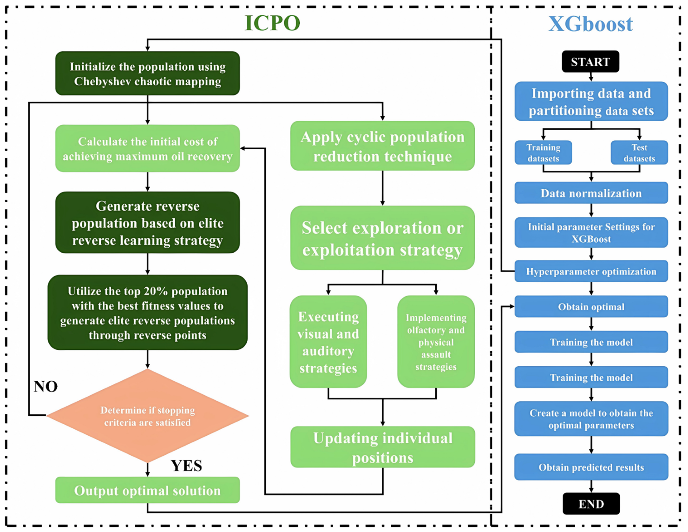Figure 4 illustrates the workflow of the CPO-XGBoost algorithm, and the optimization process can be summarized as follows:

• Data Preprocessing: The dataset is divided into training and testing subsets, and input features are normalized to eliminate dimensional biases and improve model stability.
• Population Initialization: Multiple candidate solutions, each representing a combination of hyperparameters, are randomly generated. Their fitness values are then evaluated to initialize the population.
• Iterative Optimization: The CPO algorithm iteratively updates the population using a four-stage defensive strategy:
  • First Defense Phase: Enhances solution diversity and broadens the search range by adjusting the distance between the predator and the target point, incorporating random perturbations.
  • Second Defense Phase: Simulates auditory defense behavior to improve local search capability and diversify solutions.
  • Third Defense Phase: Combines local perturbations with regional expansion to enhance global search capability.
  • Fourth Defense Phase: Simulates elastic collisions, avoiding local optima and improving global search efficiency.

Figure 4. Workflow of the CPO-XGBoost algorithm for hyperparameter optimization.

Figure 4. Workflow of the CPO-XGBoost algorithm for hyperparameter optimization.

The specific computational methods for each phase are as follows [37]:

• First Defense Phase: This phase enhances solution diversity and expands the search range by adjusting the distance between the predator and the target point, incorporating random factors. The update formula is:

$$\overrightarrow{x_i^{t+1}}=\overrightarrow{x_i^t}+{\tau }_1\times \left|2\times {\tau }_2\times \overrightarrow{x_{CP}^t}-{\displaystyle \frac{\overrightarrow{x_1}+\overrightarrow{x_r}}{2}}\right|$$

(9)

2.

Second Defense Phase: Simulating the porcupine’s auditory defense behavior, this phase enhances local search capability and further diversifies solutions. The update formula is:

$$\overrightarrow{x_i^{t+1}}=\left(1-\overrightarrow{U_1}\right)\times \overrightarrow{x_i^t}+\overrightarrow{U_1}\times \left(\overrightarrow{y}+{\tau }_3\times \left(\overrightarrow{x_{r_1}^t}-\overrightarrow{x_{r_2}^t}\right)\right)$$

(10)

3.

Third Defense Phase: This phase improves global search capability by combining local perturbations with regional expansion. The update formula is:

$$\overrightarrow{x_i^{t+1}}=\left(1-\overrightarrow{U_1}\right)\times \overrightarrow{x_i^t}+\overrightarrow{U_1}\times \left(\overrightarrow{x_{r_1}^{\prime }}+S_i^{\prime }\times \left(\overrightarrow{x_{r_2}^{\prime }}-\overrightarrow{x_{r_3}^{\prime }}\right)-{\tau }_3\times \overrightarrow{\delta }\times {\gamma }_t\times S_i^{\prime }\right)$$

(11)

4.

Fourth Defense Phase: This phase simulates elastic collisions to improve global search ability and avoid local optima. The update formula is:

$$\overrightarrow{x_i^{t+1}}=\overrightarrow{x_{CP}^t}+(\alpha (1-{\tau }_4)+{\tau }_4)\times \left(\delta \times \overrightarrow{x_{CP}^t}-\overrightarrow{x_i^t}\right)-{\tau }_5\times \delta \times {\gamma }_t\times \overrightarrow{F_i^t}$$

(12)

where $\overrightarrow{x_{CP}^t}$ denotes the best solution at iteration $t$; $\overrightarrow{x_i^t}$ denotes the position of the $i$-th individual at iteration $t$; $\overrightarrow{x_1}$ and $\overrightarrow{x_{\mathrm{r}}}$ correspond to the positions of two randomly selected individuals; ${\tau }_1$,${\tau }_2$,…,${\tau }_5$ are random values in $\left[\mathrm{0,1}\right]$, controlling update magnitude; $r_1$ and $r_2$ are two random integers within $[1,N]$, where $N$ is population size; ${\overrightarrow{U}}_1$ is randomly generated and contains elements that are either 0 or 1; The position of the predator is represented by $\overrightarrow{y}$, while $\overrightarrow{\delta }$ serves as a parameter to control the search direction; $S_i^{\prime }$ defines the odor diffusion factor, and $\alpha$ is the adjustment factor; $\overrightarrow{F_i^t}$ indicates the resistance experienced by individual $i$ during iteration $t$.

The CPO-XGBoost algorithm effectively improves model accuracy and generalization by optimizing hyperparameters through these defensive strategies.

3.2.2. Grey Wolf Optimization (GWO)

The GWO algorithm is a nature-inspired technique based on the hierarchical hunting behaviors of grey wolves [38]. The algorithm simulates the leadership hierarchy—alpha (α), beta (β), delta (δ), and subordinate wolves—and their cooperative hunting strategies to achieve global optimization. Each wolf adopts a search strategy according to its role, effectively avoiding local optima.

Figure 5 presents the workflow of the GWO-XGBoost algorithm. Initially, the positions of grey wolves are randomly generated, each position corresponding to a set of XGBoost hyperparameters. The fitness value of each wolf is evaluated based on the XGBoost model’s performance on the training dataset. The top three wolves are designated as alpha (α), beta (β), and delta (δ), representing the best, second-best, and third-best solutions, respectively. The remaining wolves follow their guidance to explore the global optimum. The position updates are defined as [39]:

$$D=|C\times X_p(t)-X(t\left)\right|$$

(13)

$$X\left(t+1\right)=X_p\left(t\right)-A\times D$$

(14)

where $D$ represents the distance between the current position of the grey wolf and the target prey; $X_p\left(t\right)$ denotes the position of the target prey; $X\left(t\right)$ represents the current position of the grey wolf; $A=2a{r}_1$, where $a$ is the iteration parameter (decreasing with iterations) and $r_1$ is a random number; $C=2r_2$, with $r_2$ as a random number introducing perturbations.

3.2.3. Artificial Hummingbird Algorithm (AHA)

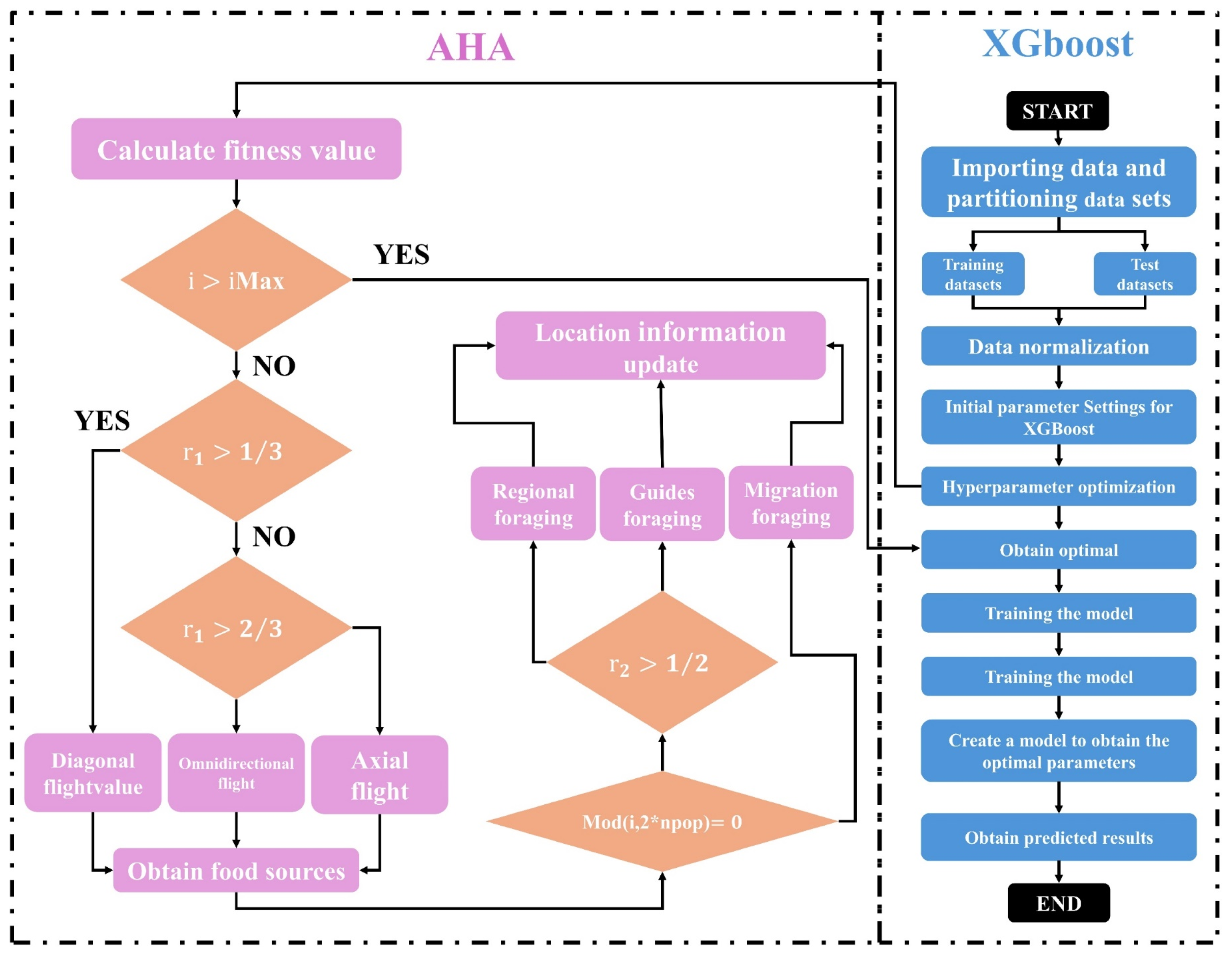
The AHA is a novel swarm intelligence optimization technique inspired by the hovering flight and dynamic foraging behavior of hummingbirds [40]. By simulating the process of hummingbirds searching for and utilizing high-quality food sources, the algorithm effectively balances global exploration and local exploitation to solve complex optimization problems. AHA uses three flight modes—axial, diagonal, and omnidirectional flight—and three intelligent foraging strategies: guided foraging, local foraging, and migratory foraging [41]. These mechanisms collectively enhance the algorithm’s ability to explore the solution space and refine candidate solutions.

As shown in Figure 6, the AHA-XGBoost algorithm begins by calculating the fitness of each hummingbird (representing a hyperparameter combination). Based on the foraging strategy and flight mode, the positions of the hummingbirds are updated, and the fitness values are recalculated. The process continues until convergence is achieved, yielding the optimal hyperparameters for the XGBoost model [42].

$$D^{\left(i\right)}=\left\{\begin{array}{c}1,\mathrm{if} i=\mathrm{rand}\left[1,d\right],\\ 0,\mathrm{else}\end{array}\right.$$

(15)

$$D^{\left(i\right)}=\left\{\begin{array}{c}1,\mathrm{if} i=P\left(j\right),j\in \left[1,d\right],P=\mathrm{rand}\left(k\right),\\ 0,\mathrm{else}\end{array}\right.$$

(16)

where $D^{\left(i\right)}$ represents the flying skill; i = rand [1, d] generates a random integer within the range [1, d], where d denotes the dimensionality of the search space; $P=\mathrm{rand}\left(k\right)$ creates a random permutation of integers from 1 to $k$; $r_1$ represents a uniformly distributed random number between 0 and 1.

3.2.4. Black Kite Algorithm (BKA)

The Black-Winged Kite Algorithm (BKA) is an optimization technique inspired by the hunting and migration behaviors of black-winged kites [43]. By combining global search strategies with local exploitation, BKA effectively addresses complex optimization problems. In the framework of the BKA-XGBoost algorithm (Figure 7), BKA optimizes the hyperparameters of the XGBoost model by iteratively improving candidate solutions. Initially, the positions of the kite population are randomly initialized, with each position corresponding to a set of XGBoost hyperparameters. The user predefines the population size and search range.

During the attack phase, BKA simulates the behavior of kites approaching their target. The positions are updated using a dynamic scaling factor ($n$) and random perturbations ($r$), ensuring a smooth transition from global exploration to local exploitation. The update formula is [44]:

$$y_{t+1}^{j,j}=\left\{\begin{array}{cc}{y}_t^{j,j}+n(2r-1)\times y_t^{j,j}& \mathrm{else}\\ y_t^{j,j}+n\left(1+\mathrm{s}\mathrm{i}\mathrm{n}\right(r)\times y_t^{j,j})& g<r\end{array}\right.,\hspace{1em}\hspace{1em}n = 0.05\times {\mathrm{e}}^{-2\times ({\displaystyle \frac{t}{T}})}$$

(17)

where $y_t^{(j,j)}$ represent the position of the $i$-th black-winged kite in the $j$-th dimension at the $t$-th iteration steps; $r$ represents a random number between 0 and 1; $g$ is a constant, often set to 0.9; $T$ represents the total number of iterations, and $t$ denotes the number of iterations completed so far.

3.3. Enhanced Algorithm

The CPO-XGBoost algorithm has demonstrated exceptional performance in optimizing CO₂-WAG development parameters for low-permeability reservoirs. Its strengths include high prediction accuracy, minimal error distribution, strong generalization ability, and excellent adaptability to complex nonlinear relationships. By effectively balancing global search and local exploitation, the algorithm mitigates overfitting and ensures consistent performance across both training and testing datasets. Additionally, it outperforms other comparative algorithms in terms of error metrics, showcasing superior stability and reliability. Detailed comparative results are presented in Section 4. However, the CPO-XGBoost algorithm has certain limitations. Its optimization process requires substantial computational resources, especially when applied to large-scale datasets, resulting in extended computation times. Furthermore, its performance is highly dependent on hyperparameter tuning, making it sensitive to configuration in complex engineering environments. This often necessitates meticulous debugging and adjustments.

To address the shortcomings of the original CPO algorithm, including slow convergence speed, suboptimal optimization performance, and low resource allocation efficiency, this study introduces two key improvement mechanisms: the Chebyshev chaotic mapping and the EOBL strategy. The Chebyshev chaotic mapping, characterized by high chaotic intensity and uniform ergodicity, effectively enhances the diversity of the initial population and prevents the algorithm from being trapped in local optima. Additionally, its nonlinear oscillatory behavior within the interval [−1, 1] improves the randomness of population initialization and global search capability. Combined with the EOBL strategy, the search efficiency and global convergence ability are further enhanced, achieving a balance between exploration and exploitation and significantly improving algorithm performance. This characteristic has been widely validated in various optimization algorithm studies as beneficial for enhancing population diversity and global search efficiency [38]. The improved ICPO algorithm increases population diversity, strengthens global search capabilities, accelerates convergence, and effectively overcomes the limitations of the original CPO algorithm.

3.3.1. Method Population Initialization via Chebyshev Chaotic Mapping

The original CPO algorithm utilizes a random initialization strategy to generate the initial population within the search space. While straightforward, this approach often results in high randomness and uneven distribution, leading to insufficient population diversity and suboptimal search performance. To address this issue, the Chebyshev chaotic mapping mechanism is introduced.

The Chebyshev chaotic mapping formula is expressed as follows [45]:

$$H(t+1)=\cos \left(p\cdot \arccos (H\left(t\right))\right)$$

(18)

$$x=a+(H(t)+1)\cdot {\displaystyle \frac{b-a}{2}}$$

(19)

where $H\left(t\right)$ represents the value of the chaotic sequence at the t-th step, which is typically distributed within the interval [−1, 1]; $p$ is the control parameter; $a$ denotes the lower bound of the search space; $b$ denotes the upper bound of the search space.

3.3.2. Elite Opposition-Based Learning Strategy for Population Optimization

A high-quality initial population is essential for accelerating convergence and increasing the likelihood of achieving a globally optimal solution. The original CPO algorithm’s reliance on random initialization often results in limited population diversity, adversely affecting convergence speed and optimization performance. To address this, the EOBL strategy is introduced during the population initialization phase. The oppositional solution is calculated as follows [46]:

$$\overrightarrow{X_{i,j}^e}=K\times (a_j+b_j)-X_{i,j}^e$$

(20)

where $K$ is a dynamic coefficient with a value range of $\left(\mathrm{0,1}\right)$; $a_j$ and $b_j$ are dynamic boundaries, which adapt to overcome the limitations of fixed boundaries. This ensures that oppositional solutions retain search experience and are less likely to get trapped in local optima.

$$\overrightarrow{X_{i,j}^c}=\mathrm{rand}(a_j,b_j)$$

(21)

To further balance global exploration and local exploitation, a nonlinear convergence factor adjustment strategy is employed. The convergence factor is updated as follows:

$$a=a_{\mathrm{initial}}-(a_{\mathrm{initial}}-a_{\mathrm{final}})\cdot \exp (t/t_{\max }-1)$$

(22)

where $a_{\mathrm{initial}}$ and $a_{\mathrm{final}}$ represent the initial and terminal values of $a$, respectively; $t$ is the current iteration number; $t_{\max }$ is the maximum number of iterations.

Compared to linear convergence, this nonlinear adjustment is more effective in balancing the demands of global and local search, thereby enhancing optimization performance and convergence speed.

3.3.3. Improved Crowned Porcupine Optimization-XGBoost Model

Building on the aforementioned enhancements, this study introduces the ICPO algorithm, which is integrated with the XGBoost model to form the ICPO-XGBoost model.

As illustrated in Figure 8, the ICPO-XGBoost model incorporates the Chebyshev chaotic mapping mechanism during the population initialization phase. This approach generates a uniformly distributed initial population, significantly enhancing diversity compared to the random initialization strategy of the original CPO algorithm. The nonlinear and periodic properties of Chebyshev chaotic mapping ensure efficient coverage of the search space, reducing the risk of local optima and improving population distribution. Following initialization, the EOBL strategy is applied to refine the population. The top 20% of individuals with the highest fitness values are used to generate an oppositional population, which is then compared with the original population. The best-performing individuals are retained as the new initial population, enhancing diversity, accelerating convergence, and increasing the likelihood of finding the global optimum. During the iterative optimization process, a nonlinear convergence factor adjustment strategy dynamically balances global exploration and local exploitation. In the early stages, the algorithm emphasizes global exploration with a larger search range to fully cover the search space. As iterations progress, local exploitation is gradually strengthened to improve optimization accuracy. Compared to linear adjustment strategies, this nonlinear approach provides greater flexibility and enhances convergence performance.

4. Results and Analysis

Accurately predicting cumulative oil production and optimizing injection-production parameters are critical for enhancing oil recovery and maximizing economic efficiency in the development of low-permeability reservoirs using CO₂-WAG injection. This chapter provides a systematic evaluation of the proposed ICPO-XGBoost model, focusing on its performance in terms of prediction accuracy, stability, and generalization capability. Through detailed comparative analyses with other mainstream algorithms, the chapter highlights the significant advantages of the ICPO-XGBoost model in addressing complex nonlinear problems. By comprehensively comparing its performance across training, testing, and validation datasets, the study validates the ICPO-XGBoost model’s reliability and superiority in practical applications. Furthermore, optimization performance tests and comparisons with traditional and state-of-the-art machine learning models further demonstrate the model’s precision and applicability. The chapter also incorporates real numerical simulation cases to systematically compare the model’s predictions with simulation results, exploring its predictive capability and applicability under various development strategies.

4.1. Comparative Analysis of Model Prediction Results

To comprehensively assess the performance of six models—XGBoost, CPO-XGBoost, AHA-XGBoost, BKA-XGBoost, GWO-XGBoost, and ICPO-XGBoost—this study utilizes the case study presented in Section 2, with a specific focus on their applicability in optimizing CO₂-WAG development parameters for low-permeability reservoirs. The dataset consists of 1225 samples, systematically divided into training, testing, and validation sets in a 5:4:1 ratio. Specifically, 613 samples are allocated for model training, 490 samples are reserved for testing, and 122 samples are used for validation. To ensure robustness and representativeness of the results, each model is independently executed 50 times, and the optimal result from each set is selected for detailed analysis.

Table 3. Hyperparameter and training settings for the four optimized models.

Model	Max Learning Rate	Learning Rate	Warm-Up Rounds	Early Stopping Rounds	Sub-Sample Ratio	Iteration Count
XGBoost	12	0.18	5	20	0.4	80
CPO-XGBoost	14	0.21	8	25	0.5	140
AHA-XGBoost	17	0.27	10	30	0.6	145
BKA-XGBoost	15	0.29	10	30	0.4	125
GWO-XGBoost	18	0.30	10	30	0.3	150
ICPO-XGBoost	15	0.35	8	25	0.5	135

summarizes the hyperparameter configurations and training settings for each model, highlighting critical factors such as model complexity, learning rate, warm-up iterations, and early stopping strategies. These configurations are meticulously fine-tuned to achieve a balance between generalization ability and mitigation of overfitting. The subsequent sections provide an in-depth analysis and comparison of the predictive performance and adaptability of these models, offering insights into their respective strengths and limitations.

The six models are evaluated based on prediction accuracy and error metrics across the training, testing, and validation datasets. Figure 9 presents the prediction values and error distributions for the six models, while Figure 10 compares the predicted values and actual values of 150 randomly selected cases from the validation dataset.

Table 4. Primary evaluation metrics for the six models.

Model	Data Range	R2	MAPE	MAE	RMSE	MSE
XGBoost	Training set	0.9343	29.54%	276.71	271.24	0.0285
	Test set	0.9321	27.68%	255.12	252.36	0.0242
	Overall data	0.9325	28.31%	279.58	273.51	0.0277
CPO-XGboost	Training set	0.9796	12.67%	131.84	127.62	0.0095
	Test set	0.9784	11.07%	126.63	105.24	0.0074
	Overall data	0.9788	12.26%	149.12	129.67	0.0081
AHA-XGboost	Training set	0.9749	16.52%	148.15	135.15	0.0119
	Test set	0.9721	15.94%	142.92	114.28	0.0088
	Overall data	0.9725	16.42%	151.45	142.61	0.0126
BKA-XGboost	Training set	0.9768	14.62%	141.51	132.82	0.0129
	Test set	0.9754	14.28%	138.87	125.95	0.0115
	Overall data	0.9758	14.59%	142.12	136.08	0.0157
GWO-XGboost	Training set	0.9632	28.42%	252.81	245.34	0.0272
	Test set	0.9627	27.33%	248.92	238.26	0.0226
	Overall data	0.9629	28.15%	256.22	245.58	0.0257
ICPO-XGboost	Training set	0.9902	10.21%	119.92	95.53	0.0072
	Test set	0.9894	8.47%	112.65	67.94	0.0053
	Overall data	0.9896	9.87%	125.63	102.98	0.0064

provide a systematic comparison of the performance of the six models across key evaluation metrics, including R², MAPE, MAE, RMSE, and MSE. The radar chart in Figure 11 visually illustrates the models’ performance across the training, testing, and overall datasets, offering a comprehensive view of their predictive capabilities.

As the baseline model, XGBoost achieves moderate prediction accuracy but demonstrates clear limitations in handling complex nonlinear relationships. The model records an overall R² value of 0.9325 and a MAPE of 28.31%. Its error distributions are broad, with significant deviations observed in both low and high-value ranges, indicating reduced generalization capability and difficulties in accurately capturing intricate data patterns. These limitations underscore the need for optimization strategies to improve the model’s performance. Among the metaheuristic-optimized models, CPO-XGBoost delivers the best results, achieving an R² value of 0.9788 and a MAPE of 12.26%, significantly outperforming the baseline XGBoost model. By effectively balancing global search and local exploitation, CPO-XGBoost excels at solving complex nonlinear problems and demonstrates robust generalization across the datasets. Its error distributions are minimal and concentrated, highlighting strong fitting accuracy and stability.

AHA-XGBoost and BKA-XGBoost also exhibit strong fitting performance, achieving R² values of 0.9725 and 0.9758, respectively. However, their error distributions are more scattered on the testing and validation sets, particularly for extreme samples. This indicates weaker generalization compared to CPO-XGBoost. Between the two, AHA-XGBoost performs slightly better due to its enhanced global search capability, achieving a MAPE of 16.42%, compared to 14.59% for BKA-XGBoost. Despite their strengths, both models show limitations in handling intricate data characteristics, as evidenced by their relatively higher MAPE values and broader error distributions. GWO-XGBoost delivers the poorest performance among the metaheuristic-optimized models, with an R² value of 0.9629 and a MAPE of 28.15%. Its broader error distributions and reduced ability to capture complex nonlinear relationships highlight its limited optimization capability, particularly in high-dimensional parameter spaces.

ICPO-XGBoost demonstrates the highest prediction accuracy and the most robust error control among all models. It achieves an R² value of 0.9896 and a MAPE of 9.87%, representing a 1.08% improvement in R² and a 19.48% reduction in MAPE compared to CPO-XGBoost. The advanced optimization strategies incorporated into ICPO-XGBoost, such as Chebyshev chaotic mapping and the EOBL strategy, significantly enhance global search capability, improve population diversity, and accelerate convergence. These enhancements enable ICPO-XGBoost to achieve superior stability, fitting accuracy, and generalization performance. The error distribution plots confirm its smaller deviations and smoother error curves, demonstrating its reliability and efficiency in accurately capturing intricate relationships between decision variables and target variables.

4.2. Performance Comparison Test of the Model

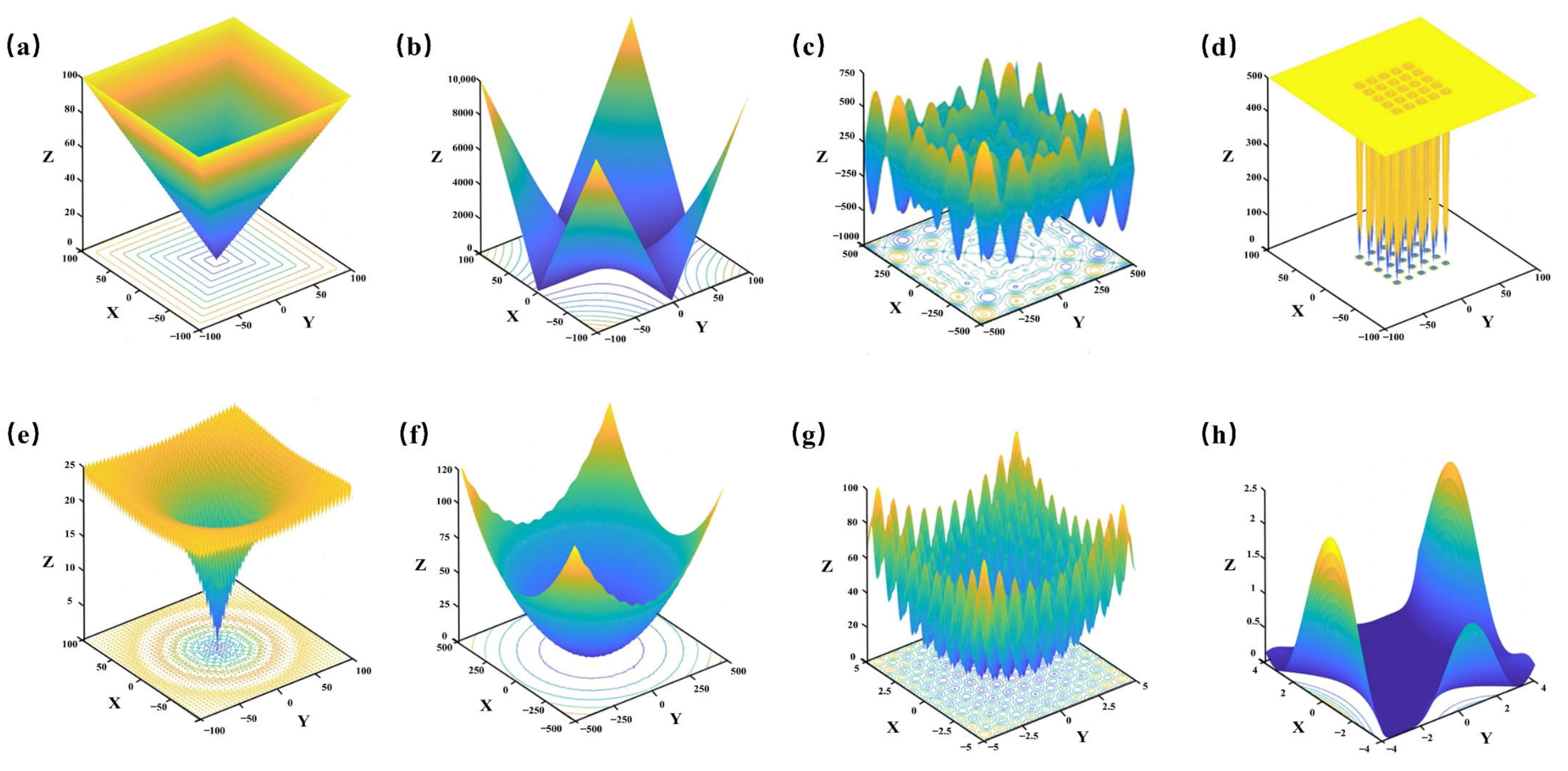
To thoroughly evaluate the optimization performance of the improved ICPO algorithm, eight benchmark test functions were selected. The specific mathematical expressions of these functions are detailed in

Table 5. Mathematical expressions of eight benchmark functions.

Function	Expression	Executions	Value Interval
F1	$f_1(x)={\max }_i\left\{\right|x_i|,1\le i\le 30\}$	30	$-100\le x_i\le 100$
F2	$f_2(x)={\displaystyle \sum _{i=1}^{30}}|x_i|+{\displaystyle \prod _{i=1}^{30}}|x_i|$	30	$-10\le x_i\le 10$
F3	$f_3(x)=-{\displaystyle \sum _{i=1}^{30}}\left(x_i\sin \left(\sqrt{\left|x_i\right|}\right)\right)$	30	$-500\le x_i\le 500$
F4	$f_4(x)={\left[{\displaystyle \frac{1}{500}}+{\displaystyle \sum _{j=1}^{25}}{\displaystyle \frac{1}{j+{\displaystyle {\sum }_{i=1}^2}{(x_i-a_{ij})}^6}}\right]}^{-1}$	30	$-65.536\le x_i\le 65.536$
F5	$f_5(x)=-20\exp \left(-0.2\sqrt{{\displaystyle \frac{1}{30}}{\displaystyle \sum _{i=1}^{30}}{x}_i^2}\right)-\exp \left({\displaystyle \frac{1}{30}}{\displaystyle \sum _{i=1}^{30}}\cos 2\pi x_i\right)+20+e$	30	$-32\le x_i\le 32$
F6	$f_6(x)={\displaystyle \frac{1}{4000}}{\displaystyle \sum _{i=1}^{30}}{x}_i^2-{\displaystyle \prod _{i=1}^{30}}\cos \left({\displaystyle \frac{x_i}{\sqrt{i}}}\right)+1$	30	$-600\le x_i\le 600$
F7	$f_7(x)={\displaystyle \sum _{i=1}^{30}}\left[x_i^2-10\cos \left(2\pi x_i\right)+10\right]$	30	$-5.12\le x_i\le 5.12$
F8	$f_8(x)=\left[1+(x_1+x_2+1{)}^2(19-14x_1+3x_1^2-14x_2+6x_1{x}_2+3x_2^2)\right]\times \left[30+(2x_1-3x_2{)}^2\right]\times \left[(18-32x_1+12x_1^2+48x_2-36x_1{x}_2+27x_2^2)\right]$	30	$-2\le x_i\le 2$

, while their respective search spaces are visualized in Figure 12. These functions include two unimodal functions (F1 and F2) and six multimodal functions (F3 to F8). Unimodal functions, which feature a single global optimum, are primarily used to evaluate the algorithm’s convergence speed and optimization accuracy. On the other hand, multimodal functions, characterized by multiple local optima, are designed to assess the algorithm’s ability to escape local optima and efficiently explore the entire search space. By combining these two types of test functions, a more comprehensive and balanced evaluation is achieved, enabling a detailed analysis of the algorithm’s accuracy, convergence efficiency, and stability, while effectively reducing the risk of becoming trapped in local optima.

Comparative experiments were conducted under identical conditions among five optimization algorithms: ICPO, CPO, GWO, AHA, and BKA. For all algorithms, the initial population size was set to 50, and the maximum number of iterations was fixed at 400. To ensure the reliability of the experimental results, each algorithm was independently executed 30 times for each test function. The evaluation criteria included the worst value, best value, mean value, and standard deviation of the results, offering a comprehensive assessment of each algorithm’s solution accuracy and stability.

Table 6. Statistical results after 30 runs of the model.

Algorithm		F1	F2	F3	F4	F5	F6	F7	F8
CPO	Worst	3.15 × 10−26	1.26 × 10−21	5.39 × 10+1	4.97 × 10+2	1.98 × 10−17	2.57 × 10−13	6.77 × 10−2	2.47 × 10+1
	Best	2.61 × 10−28	4.16 × 10−23	0.95 × 10−2	6.18 × 10+5	5.36 × 10−18	0	0	2.38 × 10+1
	Mean	5.57 × 10−27	2.10 × 10−22	8.87 × 10+1	8.47 × 10+3	8.69 × 10−17	3.64 × 10−16	1.84 × 10−3	2.43 × 10+1
	Standard	2.41 × 10−26	0.78 × 10−21	4.82 × 10+1	3.17 × 10+2	0.74 × 10−17	5.12 × 10−14	6.85 × 10−5	2.74 × 10−1
ICPO	Worst	6.15 × 10−32	3.35 × 10−30	2.76 × 10−2	7.84 × 10−4	3.61 × 10−21	1.84 × 10−21	4.75 × 10−4	3.64 × 10−1
	Best	3.57 × 10−35	7.35 × 10−33	6.94 × 10−5	6.40 × 10−6	9.74 × 10−22	0	0	3.01 × 10−1
	Mean	2.69 × 10−34	5.96 × 10−32	4.38 × 10−4	7.17 × 10−5	6.31 × 10−21	9.78 × 10−24	5.85 × 10−7	3.34 × 10−1
	Standard	4.68 × 10−32	1.12 × 10−30	0.56 × 10−2	5.23 × 10−4	2.05 × 10−21	3.67 × 10−23	3.94 × 10−9	6.31 × 10−2
GWO	Worst	4.39 × 10−21	9.28 × 10−15	6.87 × 10+8	9.71 × 10+5	2.41 × 10+1	6.86 × 10−5	2.68 × 10+6	6.41 × 10+5
	Best	3.11 × 10−23	3.35 × 10−16	2.68 × 10+5	3.85 × 10+3	8.67 × 10+0	4.65 × 10−7	8.62 × 10+3	5.11 × 10+3
	Mean	4.32 × 10−22	0.41 × 10−16	7.31 × 10+7	7.65 × 10+4	0.26 × 10+1	5.34 × 10−6	3.15 × 10+5	3.05 × 10+5
	Standard	2.94 × 10−21	2.17 × 10−15	9.65 × 10+4	8.13 × 10+5	1.51 × 10+1	5.68 × 10−6	6.95 × 10+4	2.48 × 10+5
AHA	Worst	5.73 × 10−19	7.54 × 10+0	9.71 × 10+5	3.77+12	3.41 × 10+2	3.52 × 10−2	6.67 × 10+3	2.52 × 10+3
	Best	4.47 × 10−21	5.33 × 10−1	3.99 × 10+4	9.12 × 10+11	6.64 × 10+3	6.62 × 10−5	4.97 × 10+2	2.41 × 10+2
	Mean	9.87 × 10−20	1.05 × 10−1	1.15 × 10+5	2.74 × 10+12	9.58 × 10+2	5.34 × 10−4	0.94 × 10+3	1.15 × 10+2
	Standard	4.54 × 10−19	3.67 × 10+0	6.69 × 10+5	9.74 × 10+11	2.18 × 10+2	1.22 × 10−2	3.92 × 10+2	9.75 × 10+1
BKA	Worst	2.69 × 10−30	2.16 × 10−14	5.63 × 10+3	1.42 × 10+15	7.84 × 10+1	3.69 × 10−11	3.42 × 10+5	8.59 × 10+2
	Best	8.57 × 10−31	8.75 × 10−17	7.45 × 10+1	1.01 × 10+15	2.42 × 10+0	9.77 × 10−13	7.04 × 10+1	2.78 × 10+1
	Mean	9.12 × 10−30	6.97 × 10−16	6.62 × 10+2	1.32 × 10+15	9.16 × 10+0	1.68 × 10−13	8.84 × 10+3	2.27 × 10+2
	Standard	1.58 × 10−30	1.63 × 10−14	4.36 × 10+3	1.53 × 10+14	6.15 × 10+1	8.51 × 10−11	2.91 × 10+1	2.63 × 10+2

summarizes the results obtained from 30 independent runs of each algorithm on eight benchmark functions. The results clearly demonstrate that the ICPO optimization algorithm outperforms mainstream optimization algorithms such as CPO, GWO, AHA, and BKA. For the unimodal test functions F1 and F2, ICPO achieves significantly faster convergence, higher optimization accuracy, and smaller standard deviations, highlighting its strong local search capability and stable convergence toward the optimal solution. For the multimodal test functions F3, F4, F5, and F8, ICPO exhibits exceptional stability, with its worst-case optimization results surpassing those of the other four algorithms. This underscores its superior robustness and precision in complex search spaces. Additionally, for the multimodal functions F6 and F7, ICPO performs comparably to CPO, with both algorithms consistently converging to the global optimum (objective value of 0). This demonstrates ICPO’s strong global search ability and its effectiveness in avoiding local optima.

In contrast, while CPO shows stable performance on unimodal functions, it falls slightly behind ICPO in terms of convergence speed and solution accuracy. Overall, ICPO demonstrates outstanding performance across both unimodal and multimodal benchmark functions, characterized by high accuracy, rapid convergence rates, and robust global optimization capabilities. These results underscore ICPO’s potential and competitiveness in solving a wide range of complex optimization problems.

4.3. Comparison with Previous Studies

4.3.1. Comparison with Traditional Machine Learning Models

Traditional machine learning models, such as Support Vector Machine (SVM), Random Forest (RF), K-Nearest Neighbors (KNN), Logistic Regression (LR), and Naive Bayes (NB), have been widely applied in oil and gas development strategy optimization. To validate the stability and robustness of the ICPO-XGBoost model, this study selected these models as benchmarks and conducted a detailed analysis of the performance differences between ICPO-XGBoost and traditional models from two dimensions: prediction error metrics and error distribution.

As shown in Figure 13a, ICPO-XGBoost demonstrates the best performance across all evaluation metrics, particularly achieving significantly lower RMSE and MAE values compared to other models. Additionally, its R² value is the highest, fully reflecting its outstanding fitting accuracy and strong predictive capability. In contrast, although traditional models have undergone optimization, they exhibit evident limitations in capturing complex nonlinear relationships. Notably, LR and NB models show significantly higher error metrics, indicating their poor adaptability to data structures and inability to achieve high-precision predictions. Figure 13b illustrates the relative error distribution of the models in sample predictions. The boxplot clearly shows that ICPO-XGBoost exhibits the most concentrated error distribution with the smallest interquartile range, indicating superior prediction stability and robustness, as well as minimal sensitivity to outliers. By comparison, the error distributions of the other models are notably wider, with multiple outliers, revealing greater prediction uncertainty. ICPO-XGBoost significantly outperforms traditional methods in prediction accuracy, stability, and the ability to learn complex data structures. By integrating advanced feature extraction mechanisms and optimization strategies, the proposed model not only effectively captures higher-order nonlinear patterns in the data but also substantially reduces prediction errors, enhancing its generalization ability and practical value in engineering applications.

4.3.2. Comparison with Mainstream Boosting-Based Ensemble Models

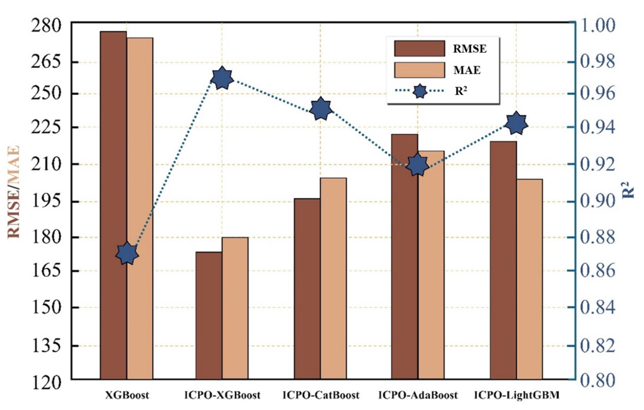
To further validate the practicality and comprehensive advantages of the proposed ICPO-XGBoost model, this study conducted a comparative analysis of its predictive performance against mainstream ensemble Boosting models, including Categorical Boosting (CatBoost), Adaptive Boosting (AdaBoost), Light Gradient Boosting Machine (LightGBM), under identical hardware conditions. As shown in the Figure 14, ICPO-XGBoost demonstrates outstanding predictive accuracy, with RMSE and MAE reduced by 38.6% and 33.8%, respectively, compared to the traditional XGBoost model. Additionally, its R² value is significantly higher than that of other models, highlighting its superior fitting precision and robust predictive capability.

In contrast, although CatBoost, AdaBoost, and LightGBM are widely recognized as leading ensemble learning methods, their performance remains inferior to ICPO-XGBoost even when combined with the ICPO optimization strategy. This performance gap can primarily be attributed to the following reasons: XGBoost’s architecture is inherently more compatible with parameter optimization methods. Its use of approximate algorithms for node splitting and regularization mechanisms strengthens the model’s responsiveness to parameter adjustments, facilitating precise optimization. On the other hand, CatBoost is primarily optimized for categorical feature processing, with complex target encoding mechanisms and symmetric tree structures that result in a less explicit parameter space, thereby limiting the ICPO algorithm’s search capabilities. Second, AdaBoost relies on an iterative mechanism of weighted weak learners, which has limited capacity for substantial performance improvements, making the optimization strategy less impactful. Although LightGBM is advantageous in terms of computational efficiency, its histogram-based feature splitting and leaf-wise growth strategy may introduce greater volatility, leading to less stable optimization effects. Under the same optimization mechanism, the structural characteristics of XGBoost are better aligned with the ICPO algorithm, enabling a synergistic effect that allows ICPO-XGBoost to excel in predictive accuracy, stability, and robustness, making it the best-performing model in this comparison.

4.4. Performance Validation of the ICPO-XGBoost Model

4.4.1. Prediction Performance and Generalization Capability Validation

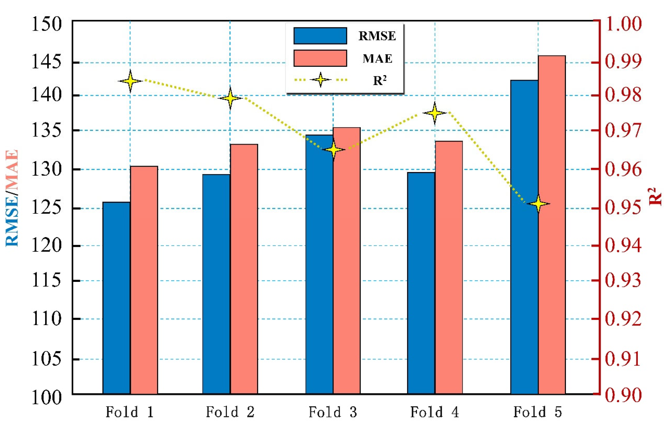
To thoroughly evaluate the predictive performance and generalization capability of the proposed ICPO-XGBoost model, this study implemented the classical five-fold cross-validation strategy as the validation framework.

Five-fold cross-validation is a widely adopted approach for model evaluation, which involves randomly partitioning the entire dataset into five approximately equal and mutually exclusive subsets (Figure 15). During each iteration, one subset is designated as the test set, while the remaining four subsets are merged to form the training set for model training and evaluation. This process is repeated five times, ensuring that each subset is used as the test set exactly once. By doing so, the method maximizes dataset utilization and effectively mitigates random errors introduced by a single data split. Upon the completion of all five folds, the test results are aggregated, and the average values of the evaluation metrics are calculated, serving as the final assessment of the model’s overall performance. The performance metrics considered include the RMSE, MAE, and the R², as illustrated in Figure 16. In the five-fold cross-validation experiment, the ICPO-XGBoost model demonstrated outstanding performance, with average metrics of RMSE = 129.35, MAE = 135.41, and R² = 0.976. The evaluation results further reveal that the variation in metrics across the five folds was minimal, with RMSE and MAE exhibiting narrow ranges of fluctuation, and R² consistently approaching 1. These findings highlight the model’s ability to maintain stable and high-quality performance under varying data partitioning scenarios, reflecting its strong robustness and excellent generalization capacity.

4.4.2. Reliability Validation

To validate the reliability of the ICPO-XGBoost model, six new development cases were designed using the LHS method based on the tNavigator numerical simulation platform, with cumulative oil production serving as the validation benchmark. A comparison between the ICPO-XGBoost model predictions and the numerical simulation results is presented in

Table 7. Parameters and results of six development strategies.

Parameter	Unit	Case1	Case2	Case3	Case4	Case5	Case6
BHPO	MPa	18.5	17.3	18.4	17.6	17.5	16.6
WGR	%	30	85	87	90	45	90
ORAT	m3/d	82.73	89.85	42.01	44.85	78.45	82.73
RATEG	m3/d	29,940.96	38,116.19	39,678.19	33,328.05	38,912.61	39,940.96
RATEW	m3/d	45.38	41.47	41.16	56.77	51.04	52.35
IC	Day	122.27	184.55	106.01	61.52	113.28	82.27
Simulation prediction	×106 m3	1.308	1.348	1.424	1.495	1.881	2.355
Model prediction	×106 m3	1.311	1.349	1.421	1.494	1.881	2.355

. The analysis demonstrates that the ICPO-XGBoost model predictions are highly consistent with the numerical simulation results, with errors controlled within ±2%.

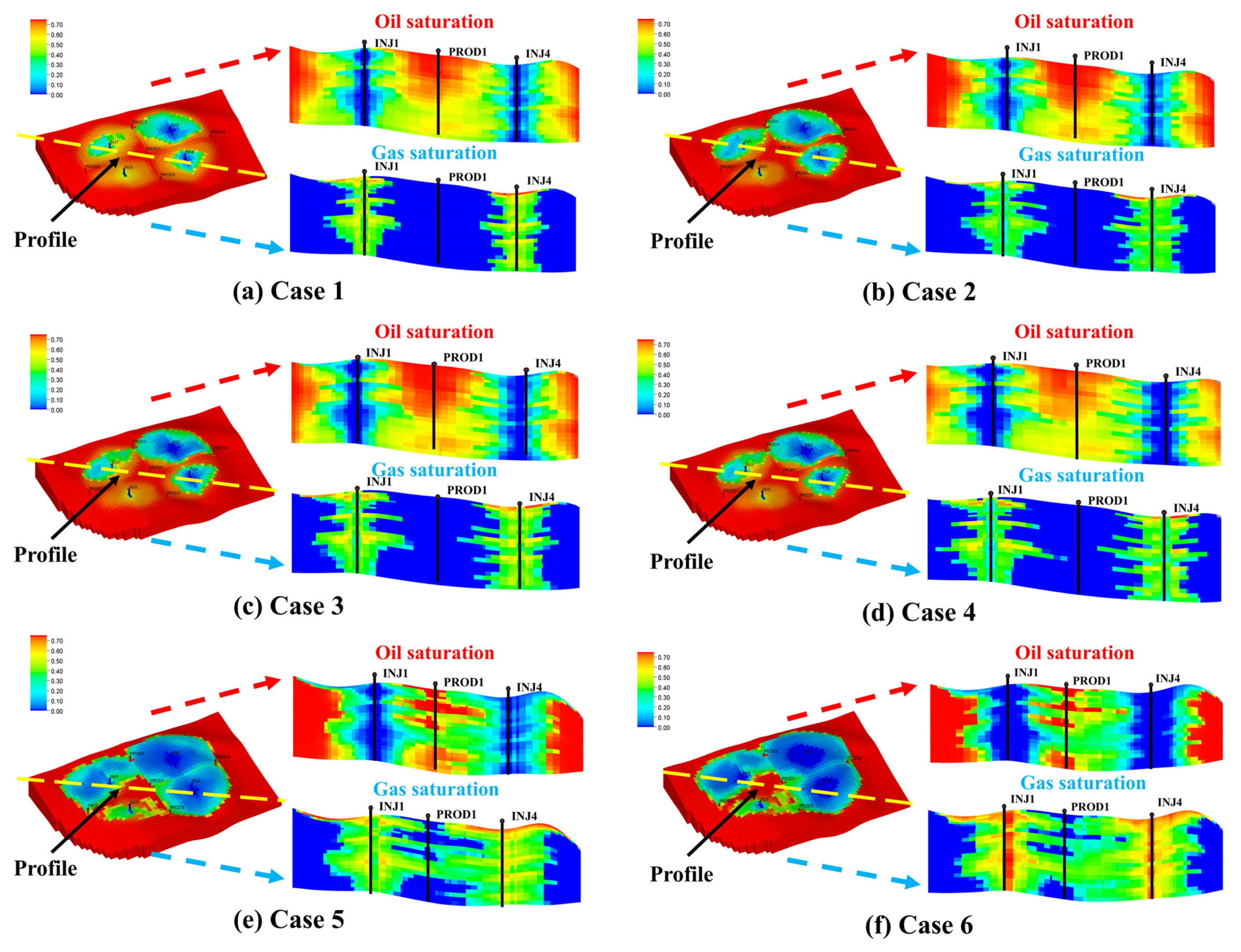
Figure 17 visually illustrates the numerical simulation results of the six development scenarios. The oil and gas saturation profiles reveal the internal fluid distribution characteristics of the reservoir and the development effectiveness under different strategies. The results indicate that scenarios with higher cumulative oil production are often associated with a higher risk of gas channeling. For instance, in Case 6, although the cumulative oil production reaches the highest value (2.355 × 10⁶ m³), severe gas channeling significantly undermines the stability of the strategy.

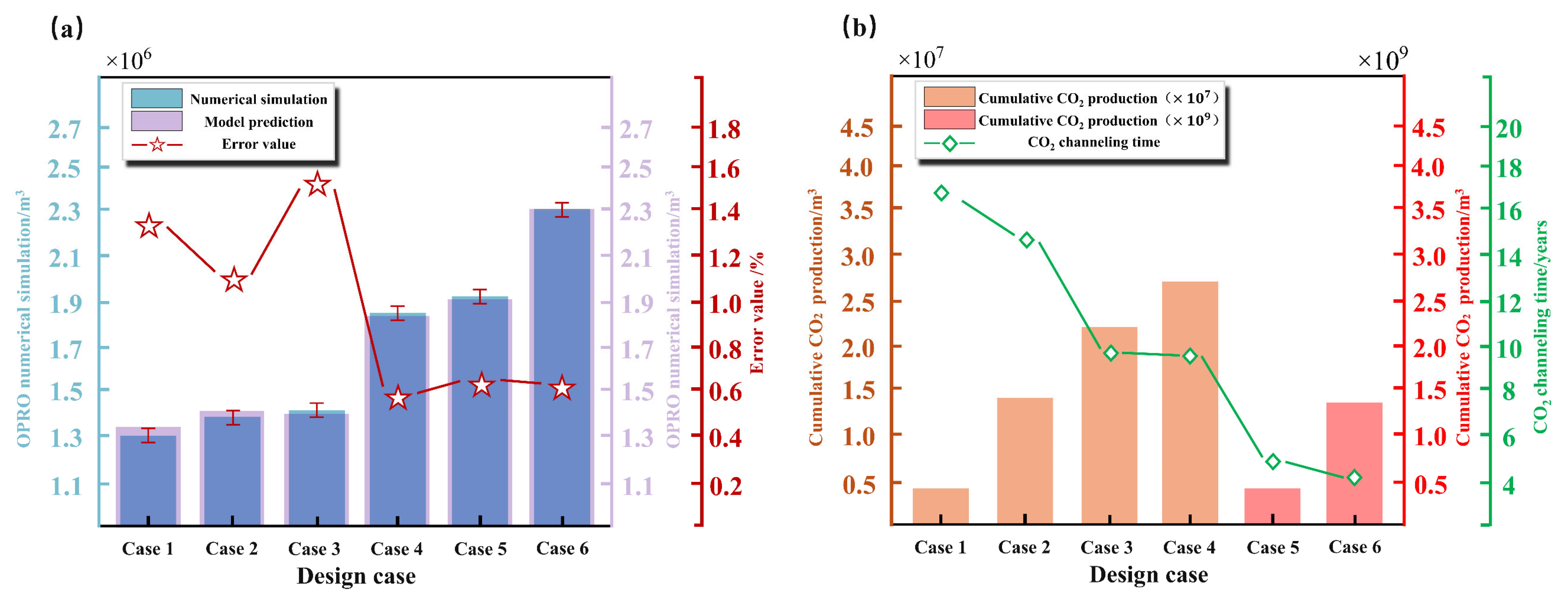
Figure 18 compares the ICPO-XGBoost model predictions with the numerical simulation results. It shows that the model predictions are in excellent agreement with the simulation results across all cases, with minimal errors that exhibit a consistent pattern. And further compares the trends of cumulative CO₂ production and gas breakthrough time. The results reveal significant differences in cumulative CO₂ production across the different development strategies, while gas breakthrough time serves as a strong indicator of gas channeling risks. For example, in Cases 3 and 5, the relatively short gas breakthrough times suggest higher gas channeling risks during the later stages of development.

4.4.3. Training Performance Analysis

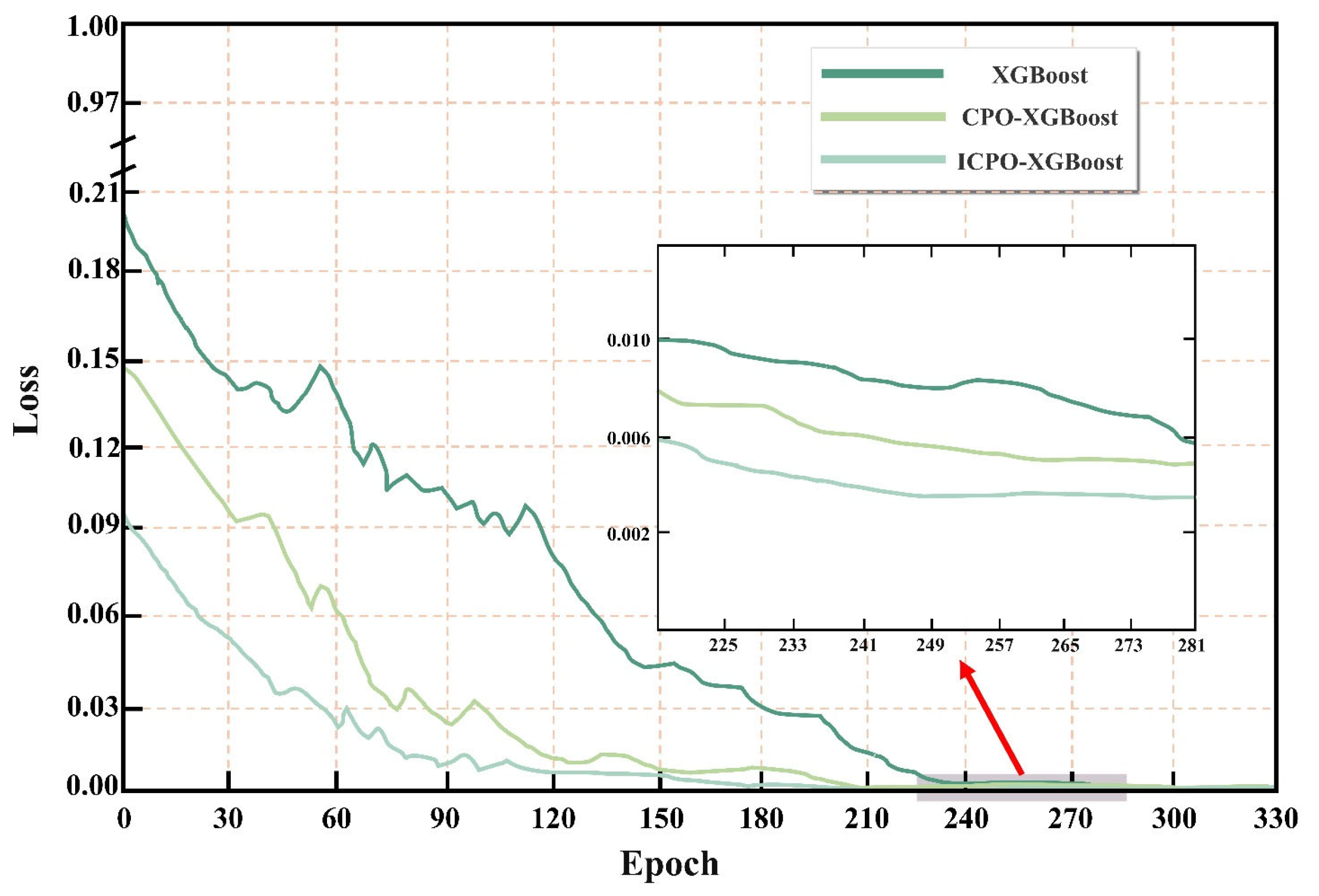
To quantitatively evaluate the performance of the ICPO algorithm during training, this study compared the loss function reduction trends of the XGBoost, CPO-XGBoost, and the proposed ICPO-XGBoost models during the training phase (see Figure 19). Results show that ICPO-XGBoost significantly outperforms the other two models in terms of loss reduction speed, particularly within the first 100 training epochs, where it completes the primary error compression phase, reducing the loss value from approximately 0.21 to near 0.05. This demonstrates superior convergence efficiency. In contrast, the loss reduction process of XGBoost and CPO-XGBoost is notably slower, and their loss values remain relatively high during the later stages of convergence. By the 60th to 80th training epochs, ICPO-XGBoost had already reduced the training loss to below 0.03, showcasing its significant performance advantage. Furthermore, the magnified local region in the figure provides a detailed comparison of the stability of the three models during the convergence phase. It can be observed that the loss curve of ICPO-XGBoost approaches zero with minimal fluctuation in the later stages of training, whereas the loss curves of XGBoost and CPO-XGBoost still exhibit noticeable oscillations. This indicates that the proposed model not only achieves faster convergence but also effectively avoids overfitting and oscillations during training. Notably, ICPO-XGBoost requires approximately 30–40% fewer training epochs to reach convergence, significantly reducing training time and computational resource consumption. These results demonstrate that ICPO-XGBoost outperforms the comparison models in both training efficiency and overall performance.

4.5. Feature Importance Analysis

To further understand the predictive behavior of the ICPO-XGBoost model, this study employs the Shapley Additive Explanations (SHAP) method to perform a global feature importance analysis on the dataset. The SHAP method quantifies the contribution of each feature to the model’s predictions by calculating the mean absolute Shapley value for each feature, thereby providing insight into the “black-box” nature of the model. Figure 20a illustrates the importance of each feature and their respective contributions to the OPRO.

Among all the features, WGR is identified as the most critical parameter, accounting for 45.12% of the total SHAP values. This finding is not only statistically validated but also aligns closely with the complex physical displacement mechanisms inherent in CO₂-WAG technology. WGR directly determines the ratio of injected water and gas, which significantly influences the displacement efficiency of the injected fluids. At low WGR values (water-dominated injection), the higher viscosity of water improves volumetric sweep efficiency, mitigates premature gas breakthrough, and enhances reservoir utilization. Conversely, excessively high WGR values (over-dominance of water injection) may lead to non-uniform fluid flow, reduced gas displacement efficiency, and even water flooding near the injection wells. Furthermore, WGR plays a critical role in suppressing gas channeling. In highly heterogeneous reservoirs where gas channeling risks are elevated, an appropriate increase in WGR (i.e., a higher proportion of water injection) can create a water barrier to block high-permeability pathways, thereby significantly improving vertical sweep efficiency. In addition to WGR, RATEW and ORAT are identified as the second and third most important features, contributing 22.37% and 19.54%, respectively. The importance of RATEW highlights the role of water injection rates in maintaining reservoir pressure and optimizing displacement performance. Optimal RATEW values ensure effective pressure support while minimizing the risk of water flooding. In contrast, features such as RATEG, BHPO, and IC exhibit relatively lower importance but still have measurable impacts on reservoir performance. The SHAP values of RATEG indicate that increasing the gas injection rate positively influences displacement efficiency during the early stages of gas injection; however, its effect is less significant compared to WGR and RATEW, as gas displacement efficiency is largely regulated by WGR and reservoir heterogeneity. The influence of BHPO is primarily associated with pressure control during injection, and its relatively lower importance suggests that the model relies more on the improvement of fluid distribution and displacement efficiency rather than solely on pressure variations. IC primarily impacts reservoir performance through its indirect regulation of displacement mechanisms across different injection-production cycles.

Figure 20b presents the distribution of SHAP values for each feature, providing further insights into their specific impacts on prediction outcomes. For instance, the SHAP values of RATEG and RATEW are predominantly positive, indicating that increasing these variables has a favorable effect on predicting cumulative oil production, particularly when injection rates are optimized within a certain range. In contrast, WGR exhibits a polarized SHAP value distribution: lower WGR values have a clear positive impact on cumulative oil production predictions, consistent with their role in improving sweep efficiency and suppressing gas channeling. However, higher WGR values tend to have a significant negative impact, likely due to reduced gas displacement efficiency and increased water flooding risks. This characteristic further validates WGR’s critical role in balancing displacement efficiency and gas channeling control.

Through comprehensive model comparisons and performance analysis, the ICPO-XGBoost model has demonstrated outstanding capabilities in optimizing CO₂-WAG processes for low-permeability reservoirs. With high predictive accuracy (R² = 0.9896) and low error rates (MAPE = 9.87%), the model significantly outperforms alternative approaches. By incorporating Chebyshev chaotic mapping and the Elite Opposition-Based Learning (EOBL) strategy, the model effectively enhances global search capability and optimization efficiency.

5. Conclusions

• This study introduces a novel ICPO-XGBoost model tailored to address the complexities of development parameter optimization and production forecasting in CO₂-WAG processes for low-permeability reservoirs. By integrating the ICPO algorithm with the XGBoost machine learning framework, the model achieves remarkable improvements in predictive performance and optimization efficiency. Key advancements, such as the incorporation of Chebyshev chaotic mapping and the EOBL strategy, significantly enhance the algorithm’s global search capability, convergence rate, and robustness.
• The ICPO-XGBoost model exhibits exceptional predictive accuracy, with an R² of 0.9896 and prediction errors constrained within 2%. These results surpass those of traditional machine learning methods and mainstream boosting-based algorithms. Comparative analyses across six metaheuristic-based optimization models further validate its superior capability in handling high-dimensional, complex parameter spaces. Benchmark function tests demonstrate the algorithm’s robustness in both unimodal and multimodal optimization scenarios.
• The SHAP-based analysis highlights the WGR as the most influential factor (45.12%) in cumulative oil production, with effective WGR control key to suppressing gas channeling and improving efficiency. RATEW and ORAT also enhance production, while BHPO shows a modest negative effect, guiding optimization strategies. The ICPO-XGBoost model is a robust, efficient tool for optimizing CO₂-WAG processes in low-permeability reservoirs, with strong generalization. Future work should extend its application to diverse reservoirs and incorporate additional constraints for greater accuracy.