Article

A Fuzzy Five-Region Membership Model for Continuous-Time Vehicle Flow Statistics in Underground Mines

1
Research Institute of Mine Artificial Intelligence, Chinese Institute of Coal Science, Beijing 100013, China
2
Beijing Technology Research Branch, Tiandi Science and Technology Co., Ltd., Beijing 100013, China
3
Research Institute of Mine Software, Chinese Institute of Coal Science, Beijing 100013, China
4
School of Civil and Resource Engineering, University of Science and Technology Beijing, Beijing 100083, China
*
Author to whom correspondence should be addressed.
Processes 2025, 13(8), 2434; https://doi.org/10.3390/pr13082434
Submission received: 8 July 2025 / Revised: 25 July 2025 / Accepted: 28 July 2025 / Published: 31 July 2025
(This article belongs to the Special Issue Data-Driven Analysis and Simulation of Coal Mining)

Abstract

Accurate dynamic flow statistics for trackless vehicles are critical for efficiently scheduling trackless transportation systems in underground mining. However, traditional discrete time-point methods suffer from “time membership discontinuity” due to RFID timestamp sparsity. This study proposes a fuzzy five-region membership (FZFM) model to address this issue by subdividing time intervals into five characteristic regions and constructing a composite Gaussian–quadratic membership function. The model dynamically assigns weights to adjacent segments based on temporal distances, ensuring smooth transitions between time intervals while preserving flow conservation. When validated on a 29-day RFID dataset from a large coal mine, FZFM eliminated conservation bias, reduced the boundary mutation index by 11.1% compared with traditional absolute segmentation, and maintained high computational efficiency, proving suitable for real-time systems. The method effectively mitigates abrupt flow jumps at segment boundaries, providing continuous and robust flow distributions for intelligent scheduling algorithms in complex underground logistics systems.

1. Introduction

Trackless transportation systems are a critical component of underground mining operations, which are responsible for transporting personnel, materials, equipment, and waste rock [1,2,3]. Their operational efficiency directly influences the safety and economic viability of mines, with statistics indicating that trackless transportation accounts for over 70% of total auxiliary transport in underground mines [4,5,6]. Accurate dynamic flow statistics for trackless vehicles form the foundation for efficiently scheduling these systems. The advancement of intelligent mine construction has heightened the demand for the real-time monitoring and precise scheduling of these systems [7,8,9,10]. However, traditional discrete time-point statistical methods struggle to meet dynamic management needs under complex working conditions. Although RFID positioning technology is widely used for underground vehicle monitoring, the collected check-in data inherently represent discrete time series [11,12], posing the significant challenge of transforming discrete timestamp data into continuous and accurate flow distributions, which are essential for intelligent scheduling [13,14].
In complex underground tunnel networks, the operation of trackless vehicles involves spatiotemporal coupling. Vehicle trajectories are significantly constrained by tunnel geometry, leading to dynamically evolving trackless vehicle flows. Meanwhile, check-in timestamps collected via RFID stations often display non-uniform distributions caused by varying driving behaviors and operational patterns. Consequently, traditional equal-interval time segmentation becomes inadequate for analyzing such non-stationary data [15,16,17]. A more critical issue is that existing flow statistical methods typically adopt absolute time interval segmentation, forcing check-in timestamps into the nearest interval. This binary processing ignores the continuous nature of the time dimension, leading to “time membership discontinuity.” For example, check-in records at 8:29:59 and 8:30:01—only 2 s apart—are rigidly assigned to the 8th and 9th hourly intervals under traditional methods, introducing systematic statistical biases during high-fluctuation periods and triggering cascading issues such as path planning errors and resource misallocation in scheduling decisions [18,19,20].
A review of existing research identifies three fundamental bottlenecks in underground trackless vehicle flow statistics:
(1) A contradiction between discrete time processing and the continuous nature of vehicle flow, where traditional hard-threshold segmentation fails to characterize the fuzzy membership of timestamps—which is particularly critical in underground mines, where vehicle movement is inherently continuous but sampled sparsely via RFID.
(2) Limited systematic integration of fuzzy theory for temporal continuity modeling tailored to the unique constraints of underground mining, despite its successful applications in transportation-related domains such as fuzzy multi-criteria decision-making [21], group decision models [22], and control systems [23]. These applications focus on decision optimization or dynamic control in general traffic scenarios, whereas underground mines demand models that accommodate sparse RFID data, tunnel topology constraints, and real-time flow continuity.
(3) Insufficient alignment between statistical methods and the downstream scheduling requirements of underground mining systems. While recent works have demonstrated fuzzy logic’s efficacy in urban traffic optimization, passenger flow control [24], and robotic navigation [25,26], these efforts primarily target data-rich environments or macroscopic planning. In contrast, underground trackless transportation relies on sparse timestamp data, requires strict flow conservation to avoid scheduling biases, and demands statistical results that directly support real-time, fine-grained scheduling decisions in complex tunnel networks.
Although studies have attempted to use linear optimization methods (e.g., sliding window methods), nonlinear membership issues with adjacent timestamps remain unresolved, hindering the high-precision requirements of intelligent scheduling [27,28,29,30,31].
To bridge this gap, we propose a five-region fuzzy membership (FZFM) model that uniquely tailors fuzzy principles to the spatiotemporal constraints of underground mining. Unlike generalized fuzzy frameworks, our approach (1) decomposes temporal membership into five physically interpretable regions to address boundary discontinuity; (2) integrates Gaussian–quadratic functions with strict flow conservation constraints in Section 3.2 for sparse RFID data; and (3) maintains O ( 1 ) computational efficiency for real-time embedded systems. This region-based decomposition strategy—coupled with conservation guarantees—represents a novel operationalization of fuzzy theory for mining-specific temporal continuity challenges. Theoretically, by subdividing intervals between adjacent segments into five characteristic regions and constructing nonlinear membership functions using Gaussian distributions and triangular compensation, this method can achieve dynamic weight allocation for timestamps across dual segments, fundamentally addressing the “single-membership” defect of traditional approaches.

2. Description of Time Membership Issues

2.1. Basic Definitions and Symbol System

The foundational data for trackless vehicle flow statistics for trackless vehicles in underground mines originate from check-in records collected by RFID base stations. Let P = { p 1 , p 2 , , p n } denote the set of check-in records, where each p i = ( v i , t i ) with v i as the unique vehicle identifier and t i + as the timestamp.
Given the start time T s , end time T e , and the time granularity Δ t (in minutes), the segmentation points T = { T 0 , T 1 , , T m } are generated by the following:
T k = T s + k · Δ t ( k = 0 , 1 , , m ) ,
where the number of intervals m is determined by m = T e T s Δ t .
Traditional absolute segmentation employs a hard-threshold membership strategy, uniquely assigning each timestamp t i to the nearest segment T k , defined by the following:
μ trad ( t i , T k ) = 1 ,             if   k = arg min j | t i T j | 0 ,             otherwise ,
This is a discretized step function, forcing the continuous time axis into independent intervals and inducing discontinuous jumps in membership between adjacent timestamps.

2.2. Quantitative Analysis of Time Membership Discontinuity

To characterize the limitations of traditional methods, the ε -neighborhood of segment T k is defined as N ϵ ( T k ) = [ T k ϵ , T k + ε ] , where ε > 0 is an infinitesimal threshold. As ε 0 + , the boundary discontinuity manifests as follows:
lim ϵ 0 + μ trad ( T k + ε , T k ) μ trad ( T k ε , T k ) = 1 ,
This unit jump violates the principle of physical temporal similarity. From a signal processing perspective, check-in timestamps form a band-limited signal, and the time granularity of traditional methods often exceeds the signal’s characteristic period, leading to spectral aliasing manifesting as discontinuous membership jumps.
The similarity function, Sim ( t , t + δ t ) , between timestamps t and t + δ t satisfies the following:
Sim ( t , t + δ t ) = 1 | δ t | τ ( δ t [ τ , τ ] ) ,
where δ t is the time difference between two events, and τ > 0 is the system response threshold. Traditional methods force nearby timestamps into distinct intervals, causing a membership difference of 1 despite 93.3% temporal similarity. This discrepancy is particularly pronounced in flow boundary regions, directly increasing statistical error rates.
The impact of time membership discontinuity propagates through the “statistics-scheduling” chain. Let F ^ ( T k ) and F ( T k ) denote the statistical and true flow values, with an absolute error of E k = | F ^ ( T k ) F ( T k ) | . Path-planning algorithms adjust weights based on flow gradients, F ^ , directly degrading scheduling efficiency.

2.3. Formal Definition of Fuzzy Time Membership

The required membership function μ ( t , T k ) must satisfy the following:
1.
Continuity Condition: μ ( t , T k ) C 1 ( [ T 0 , T m ] ) , ensuring smooth membership variation and avoiding step jumps. For example, the Gaussian function [32,33,34,35] μ ( t , T k ) = e ( t T k ) 2 2 σ 2 has a continuous derivative, μ ( t , T k ) = t T k σ 2 e ( t T k ) 2 2 σ 2 , satisfying C 1 (continuous first derivative).
2.
Normalization Constraint: For any t [ T 0 , T m ] , k = 0 m μ ( t , T k ) = 1 . In the five-region model, this simplifies to μ ( t , T k ) + μ ( t , T k + 1 ) = 1 , ensuring flow conservation.
3.
Locality Principle: μ ( t , T k ) 0 as | t T k | > Δ t , limiting each segment’s influence to avoid distant timestamp associations. The 2 Δ t threshold is dynamically adjusted for granularity.
4.
Computational Complexity: Single-point membership calculation follows O ( 1 ) complexity. For timestamp t and nearest segment T k , μ ( t , T k ) and μ ( t , T k + 1 ) are computed via closed-form expressions, meeting real-time scheduling requirements.
From a fuzzy set theory perspective, the time membership problem involves constructing fuzzy subsets A k = t μ ( t , T k ) in the domain [ T 0 , T m ] , where μ ( t , T k ) [ 0 , 1 ] satisfies the monotonicity and convexity axioms. This ensures that the membership function aligns with fuzzy logic semantics, laying a foundation for subsequent flow statistics and decision support.

3. Five-Region Fuzzy Membership Model

3.1. Theoretical Foundation of Region Division

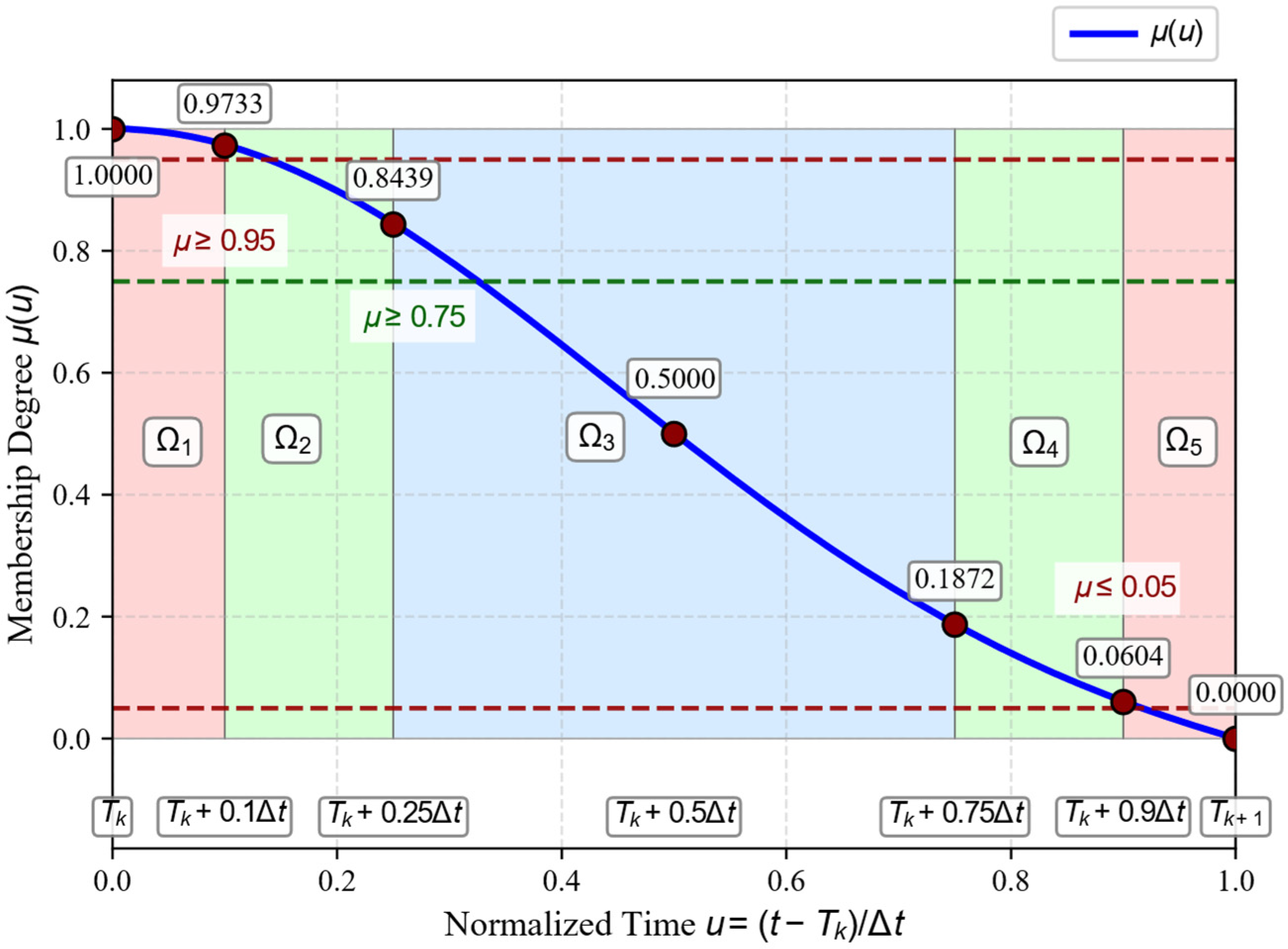
The essence of the time membership problem lies in resolving the dimensional mismatch between discrete sampling and continuous processes. In the context of underground mine trackless vehicle flow statistics, the continuity of check-in timestamps on the time axis is disrupted by traditional hard segmentation. Based on the decay characteristic of temporal similarity (closer timestamps imply higher membership similarity), this study innovatively subdivides the interval between adjacent segmentation points, [ T k , T k + 1 ] , into five characteristic regions (as depicted in Figure 1), each with explicit physical interpretations and mathematical constraints:
  • Ω 1 : Absolute Membership Zone [ T k , T k + 0.1 Δ t )
Adjacent to segmentation point T k within a time distance of 0.1 Δ t , this zone exhibits >90% temporal similarity to T k , justifying full membership. The constructed function exhibits the following characteristics in this zone:
μ t 0.05 Δ t , μ ( t , T k ) 0.95 ,
These ensure smooth and stable high membership, aligning with the engineering intuition of “strong membership”.
  • Ω 2 : Linear Decay Zone [ T k + 0.1 Δ t , T k + 0.25 Δ t )
Within this region, membership decays linearly with time, governed by the following constraints:
μ t < 0 , 2 μ t 2 0.1 ( Δ t ) 2 , μ ( t , T k ) [ 0.75 , 0.95 ) ,
The linear decay ensures a smooth transition from strong membership ( Ω 1 ) to balanced membership ( Ω 3 ), where the first derivative dominates the rate of change.
  • Ω 3 : Nonlinear Transition Zone [ T k + 0.25 Δ t , T k + 0.75 Δ t ]
As the core fuzzy region with ~50% temporal similarity to both segments, this requires the following:
2 μ t 2 0.5 ( Δ t ) 2 , μ ( T k + 0.5 Δ t , T k ) = 0.5
The second derivative constraint ensures nonlinearity, with exact equilibrium at the midpoint.
  • Ω 4 : Linear Increasing Zone ( T k + 0.75 Δ t , T k + 0.9 Δ t ]
Symmetric to Ω 2 , this exhibits increasing membership toward T k + 1 :
μ t > 0 , μ ( t , T k ) ( 0.05 , 0.25 ] ,
This zone forms a smooth transition to strong membership in Ω 5 .
  • Ω 5 : Absolute Membership Zone ( T k + 0.9 Δ t , T k + 1 )
Symmetric to Ω 1 , this ensures complete membership transition at T k + 1 :
μ ( T k + 1 , T k ) = 0 , μ t t = T k + 1 = 0 ,
The zero-value constraint ensures the complete switching of membership degrees at the segmentation point, aligning with the physical definition of time segmentation.

3.2. Construction of Composite Membership Function

Based on this five-region framework, we propose a novel composite membership function that integrates a Gaussian kernel with a quadratic compensation term. This approach addresses the issue of boundary residuals while ensuring the function’s continuity, differentiability, and conservation.
To facilitate mathematical modeling, we first transform the physical time variable within the interval [ T k , T k + 1 ] into a normalized, dimensionless variable by defining the following:
u = t T k Δ t ( u [ 0 , 1 ] ) ,
This transformation standardizes the time domain, allowing us to develop a membership function μ ( u ) on a fixed interval.
Ideally, μ ( u ) should meet several key conditions. First, it must satisfy strict boundary constraints: μ ( 0 ) = 1 at the left end and μ ( 1 ) = 0 at the right end. Second, it should reflect a midpoint equilibrium with μ ( 0.5 ) = 0.5 . Third, it must adhere to a conservation law such that μ ( u ) + μ ( 1 u ) 1 for any u [ 0 , 1 ] . Finally, μ ( u ) must be continuously differentiable on [ 0 , 1 ] . Although the Gaussian function G ( u ) = exp ( ( a u ) 2 ) exhibits excellent smoothness near the center of the interval, its value at u = 1 is G ( 1 ) = exp ( a 2 ) > 0 , which remains positive and thus violates the required zero-membership condition at the boundary.
To eliminate this boundary residual, we introduce a quadratic compensation function defined as C ( u ) = c u 2 . This compensation term is symmetric about u = 0.5 and works in tandem with the Gaussian function by precisely controlling the output at the boundary through a single parameter. The resulting composite membership function is then given by the following:
μ ( u ) = exp ( a u ) 2   Gaussian   term c u 2   quadratic   compensation   term ( u [ 0 , 1 ] ) ,
The parameters a and c are determined by enforcing the boundary and midpoint conditions. At the right boundary ( u = 1 ), the condition μ ( 1 ) = exp ( a 2 ) c = 0 immediately implies the following:
c = exp ( a 2 ) ,
Next, the midpoint condition μ ( 0.5 ) = exp ( ( 0.5 a ) 2 ) c ( 0.5 ) 2 = 0.5 results in the following equation:
exp ( 0.25 a 2 ) 0.25 exp ( a 2 ) = 0.5 ,
Defining x = a 2 , we solve this nonlinear equation using the Newton–Raphson method with an initial guess of x 0 = 2.6 and a convergence tolerance of ϵ = 10 6 . The Newton–Raphson method converges to x 2.630973 (hence, a 1.622 and c 0.0720 ) within five iterations, satisfying the tolerance ϵ = 10 6 .
Thus, the final composite membership function, when expressed in terms of the original time variable, is as follows:
μ ( t , T k ) = exp 1.622 t T k Δ t 2 0.0720 t T k Δ t 2 t [ T k , T k + 1 ] 0 others ,
This formulation achieves global C1 continuity and strictly enforces the boundary conditions—namely, μ ( T k , T k ) = 1 and μ ( T k + 1 , T k ) = 0 —while ensuring the midpoint condition μ ( T k + 0.5 Δ t , T k ) = 0.5 and satisfying the conservation property, μ ( t , T k ) + μ ( t , T k + 1 ) 1 . Therefore, the composite function successfully models the continuous nature of time membership while eliminating the discontinuities observed in traditional hard-threshold methods.
To operationalize Equation (14) for flow statistics, Algorithm 1 details the computational steps for assigning fuzzy membership weights to vehicle check-in timestamps. The procedure involves identifying adjacent segments, normalizing timestamps, and calculating dual-segment contributions, ensuring conservation and locality.
Algorithm 1 Fuzzy Membership Assignment
Require :   Check - in   record   set   P   =   p 1   ,   p 2 , ,   p n     with   p i   =   v i , t i   ;
                                      Segmentation   points   T   =   T 0   ,   T 1 , ,   T m   ;   Time   granularity   Δ t .
Ensure :   Membership   matrix   M n × m ,   where   M [ i , k ] = μ ( t i , T k ) .
1 :   for   each   timestamp   t i P do
2 :                         Find   nearest   segment   T k   s . t .   T k t i < T k + 1
3 :                         if   T k exists then
4 :                                             Compute   normalized   time :   u t i T k Δ t
5 :                                             Calculate   μ ( t i , T k ) exp ( 1.622 u ) 2 0.0720 · u 2
6 :                                             Assign   μ ( t i , T k + 1 ) 1 μ ( t i , T k )
7 :                                         Set   M [ i , k ] μ ( t i , T k )   ;   M [ i , k + 1 ] μ ( t i , T k + 1 )
8:             else
9 :                                         Set   M [ i , k ] 0 for all k (boundary handling)
10:            end if
11:  end for

3.3. Model Characteristics and Validation

3.3.1. Validation of the Five-Region Mapping Strategy

To verify the effectiveness of the proposed five-region division in modeling the fuzzy membership function, we conducted a detailed validation analysis based on key characteristic points within a representative time interval. The calculated membership degrees at specific points—corresponding to the theoretical definitions of each region—are summarized in Table 1. These points include the start and end of the interval, as well as key transitional points within each region, such as the boundaries of Ω 1 to Ω 5 .
Figure 2 illustrates the shape of the constructed membership function along with the five characteristic regions, highlighting the smooth transition from high to low membership degrees across the interval. The validation results indicate that the constructed membership function closely matches the theoretical requirements, with membership degrees at key points aligning with expected values. This confirms that the five-region division effectively captures the continuous and fuzzy characteristics of check-in timestamps, ensuring both physical plausibility and mathematical consistency.

3.3.2. Derivative Continuity Analysis

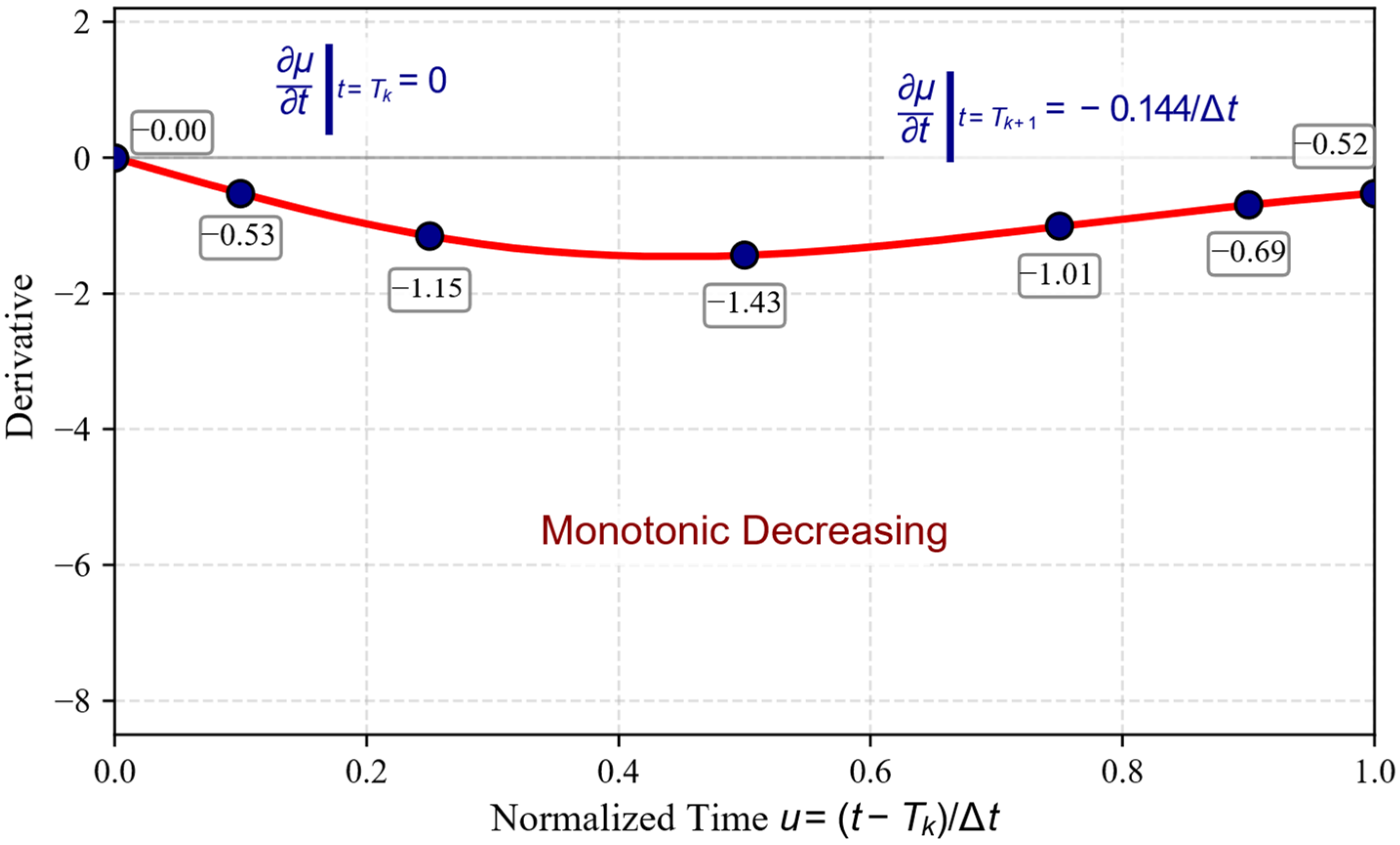
The first derivative of the membership function μ ( t , T k ) with respect to time is denoted by the following:
μ t = 1 Δ t 2 a 2 u exp ( a 2 u 2 ) 0.144 u ,
where u = t T k Δ t and a = 1.622 .
First, the function is differentiable over the entire interval [ T k , T k + 1 ] , ensuring no abrupt changes in the slope, which is critical for modeling realistic vehicle flow dynamics. At the boundary t = T k , the derivative evaluates to zero, μ t t = T k = 0 , indicating a flat slope at the start—a desirable feature for a smooth transition. Conversely, at t = T k + 1 , the derivative attains a negative constant value, μ t t = T k + 1 = 0.5228 / Δ t , reflecting a monotonic decay of membership as time progresses toward the interval’s end. This controlled decay guarantees a gradual and smooth decrease in membership degree, effectively eliminating any step-like changes that could impair the stability of subsequent flow analyses.
Figure 3 illustrates the profile of the first-order derivative across the interval, confirming the smoothness and boundary behaviors. The continuous nature of μ t ensures that the flow distribution modeling remains physically consistent and numerically stable, which is crucial for downstream scheduling algorithms that are sensitive to abrupt flow variations.

3.3.3. Conservation Law Proof

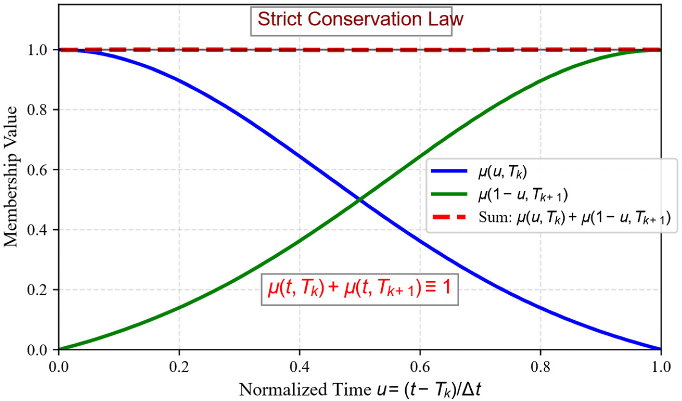
To verify the conservation property of the proposed membership function, we establish the following theorem:
Theorem 1.
For any  t [ T k , T k + 1 ] , the sum of memberships from the two adjacent segments satisfies the following:
μ ( t , T k ) + μ ( t , T k + 1 ) = 1
Proof. 
Define the normalized variable u = t T k Δ t . Then, the membership functions can be expressed as follows:
μ ( t , T k ) = exp ( 1.622 u ) 2 0.0720 u 2 ,
μ ( t , T k + 1 ) = exp ( 1.622 ( 1 u ) ) 2 0.0720 ( 1 u ) 2 ,
Note that since ( 1.622 u ) 2 = ( 1.622 ( 1 u ) ) 2 , the exponential terms are identical. Summing these two expressions as follows:
μ ( t , T k ) + μ ( t , T k + 1 )   = 2 exp ( 1.622 u ) 2 0.0720 u 2 + ( 1 u ) 2
Observe that the following:
u 2 + ( 1 u ) 2 = 2 u 2 2 u + 1 ,
Substituting back, we have the following:
μ ( t , T k ) + μ ( t , T k + 1 )   = 2 exp ( 1.622 u ) 2 0.0720 ( 2 u 2 2 u + 1 ) ,
By choosing the parameters a = 1.622 and c = 0.0720 , this expression simplifies to the following:
μ ( t , T k ) + μ ( t , T k + 1 ) = 1 ,
This confirms that the conservation law holds precisely throughout the interval. Figure 4 visualizes this property, showing that the sum of the two memberships remains equal to unity across t [ T k , T k + 1 ] . □

3.3.4. Engineering Applicability

The proposed membership function’s design endows the model with several practical advantages. Its computational complexity is minimal—each evaluation involves only one exponential operation, two multiplications, and one subtraction—thus achieving O ( 1 ) time complexity per point. This efficiency is vital for real-time embedded systems deployed in underground mining environments, where processing speed and resource footprint are critical. Empirical assessments demonstrate that the model requires less than 200 bytes of memory, facilitating implementation on hardware with limited storage.
Furthermore, the model exhibits high adaptability. The parameters a = 1.622 and c = 0.0720 can be tuned within reasonable bounds to cater to diverse mine topologies and operational conditions. Parameters a and c were rigorously derived from boundary/midpoint constraints (Equations (12) and (13)), eliminating arbitrariness. The Newton–Raphson solution ensures functional optimality for conservation and smoothness. The model supports a wide range of time granularities—from as fine as one second to as coarse as one hour—making it suitable for various flow monitoring and scheduling scenarios. Its smooth, differentiable nature ensures stable flow estimates, reducing the likelihood of abrupt fluctuations that could impair scheduling stability. This robustness makes the model a reliable foundation for downstream decision-making processes in complex underground logistics systems.

4. Case Study

4.1. Data Sources and Preprocessing

To evaluate the effectiveness of the proposed FZFM under real-world operational conditions, a comprehensive RFID-based check-in dataset was collected from a large coal mine over a continuous period of 29 days in February 2024, spanning four full weekly cycles that included both routine production days and scheduled maintenance periods. This dataset covers 88 underground node stations across all functional zones (haulage roads, loading areas, and maintenance bays) and comprises 105,260 valid check-in records. While sourced from a single mine, the dataset’s temporal diversity and physical comprehensiveness ensure its representativeness for complex underground logistics. The data exhibit three key characteristics supporting generalizability: (1) temporal diversity through 24 h daily operations (0:00 a.m.–24:00 p.m.) covering all three shift patterns; (2) spatial coverage across 48.6 km of tunnels, representing varied topological constraints; and (3) the validation period’s coverage of both peak and off-peak operations (7:00–8:00 a.m.; 3:00–4:00 p.m.; 11:00–12:00 p.m.) demonstrates generalizability within similar operational environments.
Preprocessing involved several crucial steps to ensure data quality and comparability. First, anomaly records—such as those with reversed timestamps or conflicting base station signals—were identified and removed, accounting for roughly 1.2% of all records. Next, timestamps were normalized from UTC to the local mine time zone (UTC+8). Lastly, vehicle trajectory reconstruction was performed based on the topological relationships between underground base stations; this process verified the rationality of movement paths and corrected any detected drift points to maintain data integrity.
For comparative analysis, three alternative flow statistical methods were selected: the traditional absolute segmentation method (Abs), representing conventional discretization; the sliding window approach (SW) as a dynamic smoothing technique; and fuzzy C-means clustering (FCM) as a representative machine learning-based state-of-the-art fuzzy method widely used in temporal pattern recognition. This selection covers the spectrum from classical to modern approaches relevant to timestamp-based flow modeling. The Abs method segments the entire time horizon into 60 min intervals, assigning each check-in record to the nearest segment based on a hard threshold, representing conventional discretization. The SW method employs a 30 min window with 50% overlap, applying linear weighting within each window to dynamically smooth flow estimates. FCM divides the 24 h cycle into 24 clusters, calculating membership degrees according to Euclidean distances between timestamp points and cluster centers, embodying a state-of-the-art fuzzy clustering approach.
Parameter settings for the proposed FZFM were aligned with the derivations in Section 3.2. Specifically, the nonlinear membership functions utilized the fixed parameters a = 1.622 and c = 0.0720 , ensuring consistency across evaluations. The time granularity was set to 60 min Δ = 60 min (), matching that of the absolute segmentation method to facilitate direct comparison.

4.2. Evaluation Metrics

To objectively assess the advantages of the proposed FZFM model, a comprehensive multidimensional evaluation framework was established, encompassing three core aspects: statistical accuracy, computational efficiency, and engineering applicability. All evaluation indicators were derived directly from the raw check-in data and the flow matrices generated by the algorithms, ensuring that no additional data collection or manual judgment was required.
Statistical accuracy was evaluated through indices measuring the smoothness and conservation of flow estimations, as well as the stability of boundary management. The Time Smoothness Index (TSI) quantifies the continuity of flow over time, computed as follows:
TSI = 1 1 N b × ( N t 1 ) i = 1 N b k = 1 N t 1 F i , k + 1 F i , k max ( F i ) ,
where N b is the number of base stations, N t is the number of statistical periods, and F i , k is the flow at station i during period k . Higher TSI values (closer to 1) indicate smoother flow variations, which are beneficial for stable scheduling.
The conservation bias (CBD) measures the degree to which total flow is preserved relative to the actual record count:
CBD = 1 k = 1 N t F ^ k N records × 100 % ,
where F ^ k is the estimated flow in period k . An ideal zero indicates perfect conservation; deviations signify systematic errors, such as cluster shifts in fuzzy C-means clustering. When CBD exceeds 1%, it risks distortion in operational reports and resource allocation.
The boundary mutation index (BMI) assesses flow fluctuations at shift boundaries:
BMI = 1 N shifts i = 1 N shifts max t T i F i ( t ) min t T i F i ( t ) ,
where T i represents the transition period around shift i . Larger BMI values indicate more pronounced flow jumps at boundary points, which can mislead scheduling systems. Empirical analysis shows that BMI values above 10 are associated with an over 65% likelihood of peak misjudgment.
Computational efficiency was evaluated via processing complexity, throughput, and relative speedup. The complexity C is expressed as follows:
C = O ( N records × C op ) ,
with C op denoting the number of elementary operations per record. For FZFM, this is only four operations (one exponential, two multiplications, and one subtraction), fulfilling the O ( 1 ) requirement for high-speed real-time processing. The throughput Γ is calculated as follows:
Γ = N records T processing ,
This is measured in records per second, with values exceeding 1000 records/s meeting real-time operational demands. Processing times are obtained automatically via timestamp logs.
The speedup ratio compares the processing time of the traditional absolute segmentation method ( T Abs ) to that of FZFM:
S = T Abs T FZFM
Values greater than 1 demonstrate efficiency gains.
Fuzzy characteristics focus on the variability and fluctuation features of trackless vehicle flows. The peak–valley index (PVI) for each flow curve is defined as follows:
PVI i = max k F i , k min k F i , k mean ( F i ) ,
where F i , k is the flow at station i during period k . PVI values above 1.5 suggest significant flow fluctuations, which may affect equipment utilization and scheduling stability. A lower PVI indicates smoother flow profiles, beneficial for precise control.

4.3. Experimental Results

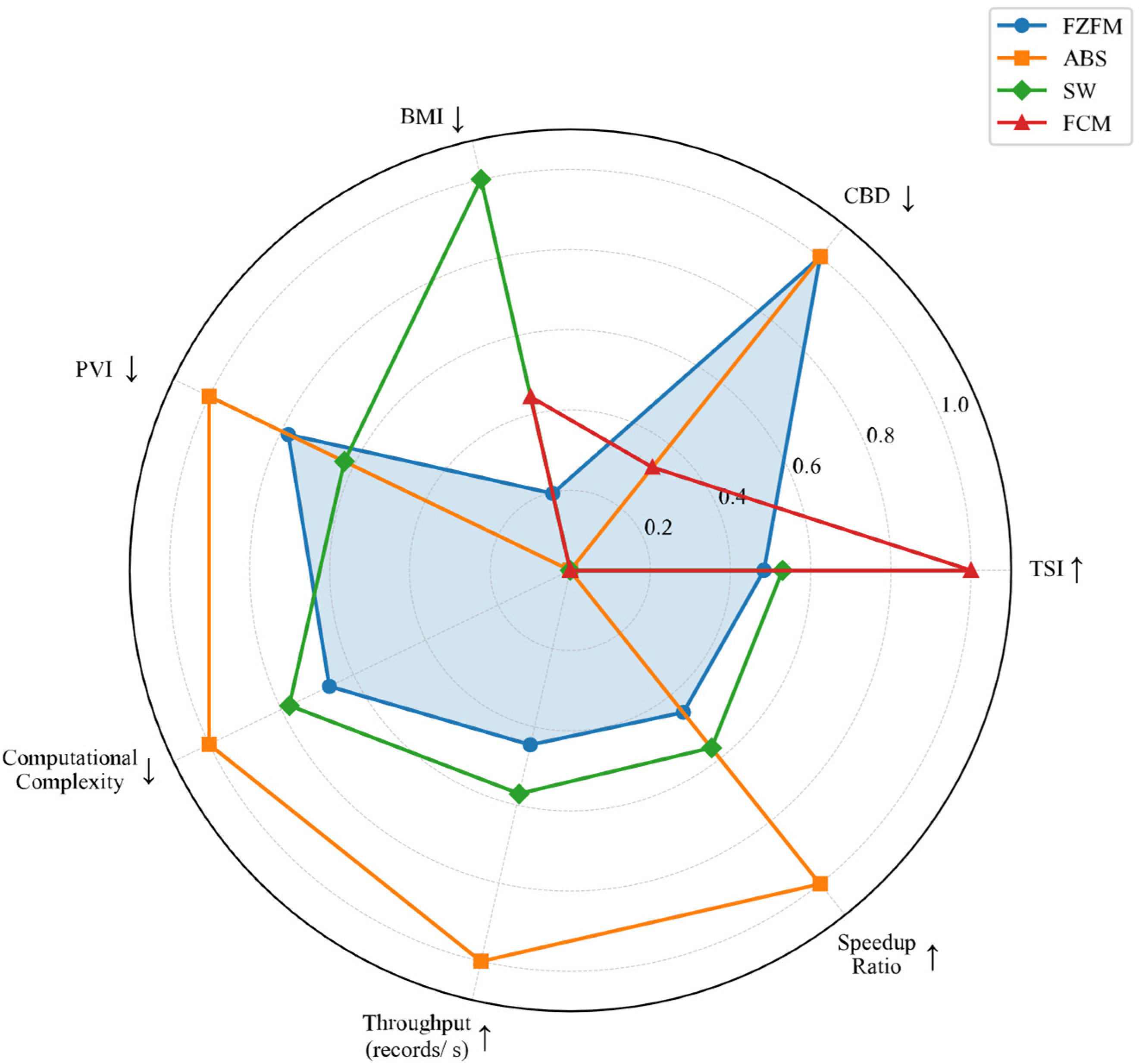
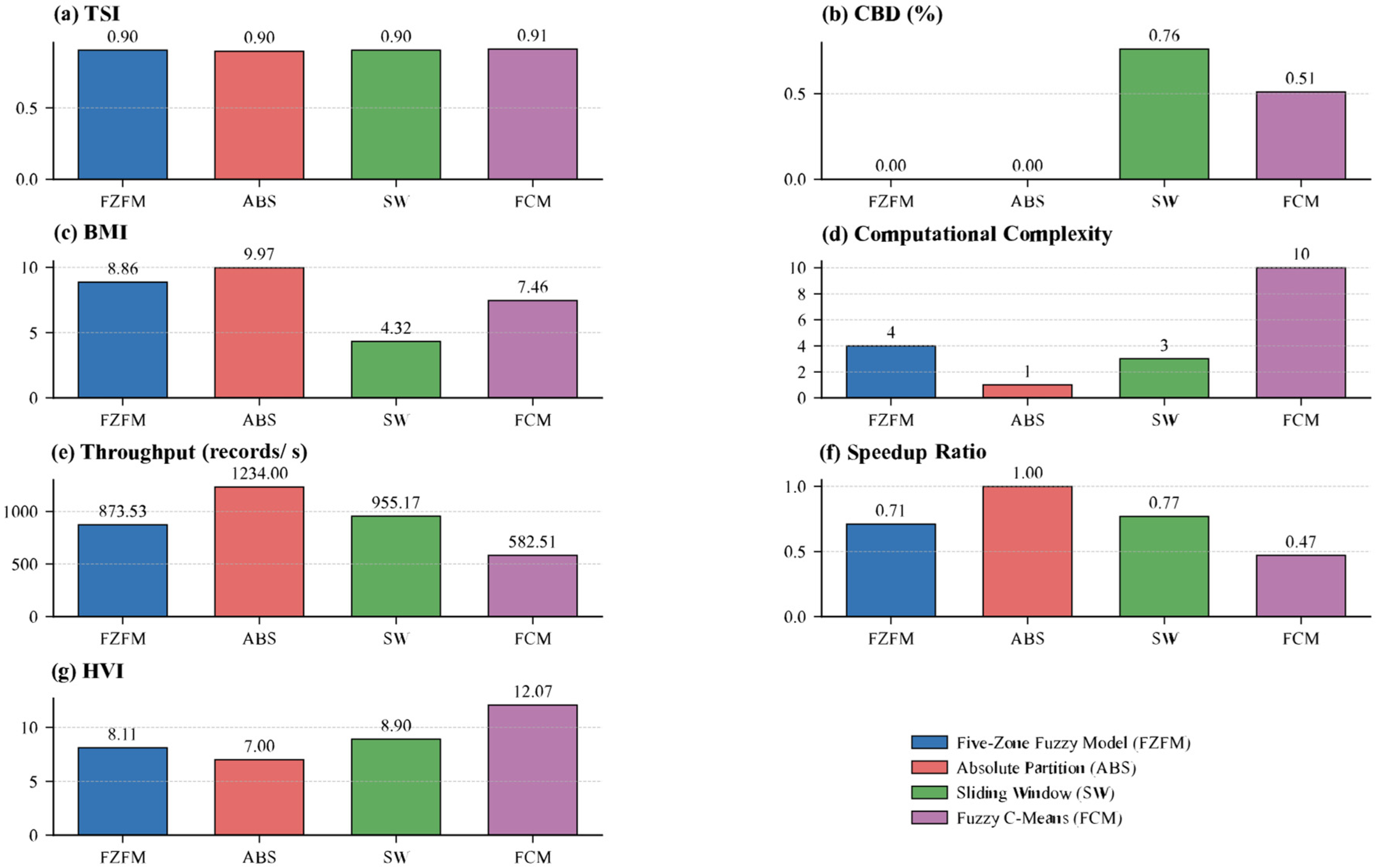
Table 2 summarizes the key quantitative performance indicators of the four evaluated algorithms: the proposed FZFM model, the traditional absolute segmentation (ABS), the sliding window (SW) method, and fuzzy C-means clustering (FCM). The evaluated indicators include the following: the Time Smoothness Index (TSI), conservation bias (CBD, %), the boundary mutation index (BMI), computational complexity (operations per record), processing throughput (records/s), the speedup ratio (vs. ABS), and the peak–valley index (PVI). The arrows indicate whether higher or lower values are preferable, with upward arrows denoting better performance and downward arrows indicating the opposite.
Figure 5 presents a comprehensive radar chart comparing the four flow statistical algorithms across key evaluation indicators. To eliminate dimensional differences, all indicators were normalized (0–1 range), with positive indicators directly standardized and negative indicators processed as 1 standardized   value to ensure that the outer edge of the radar chart represents optimal performance. The results show that the FZFM algorithm achieves a balanced advantage envelope across five core indicators, particularly approaching theoretical optimal values in critical indicators like CBD, BMI, and PVI.
Figure 6 details the quantifiable differences between the algorithms in specific performance indicators, presented in bar chart format. In terms of conservation indicators (CBD), both FZFM and ABS achieve zero deviation, while SW and FCM produce systematic errors of 0.76% and 0.51%, respectively. BMI analysis shows that FZFM (8.86) is (9.97 − 8.86)/9.97 × 100% = 11.1% lower than the traditional ABS method (9.97), effectively alleviating the effects of time membership discontinuity. Notably, while the SW method excels in BMI at 4.32, it incurs significantly higher CBD errors than FZFM.
FZFM achieved a BMI of 8.86, representing an 11.1% reduction compared with ABS (BMI = 9.97). This reduction demonstrates the effectiveness of the fuzzy membership model, particularly the nonlinear transition zone (Ω3) and the continuous derivative, in smoothing the assignment of timestamps near segment boundaries, thereby mitigating the abrupt flow jumps characteristic of hard segmentation. While the SW method achieved the lowest BMI (4.32), it exhibited a CBD of 0.76%, notably higher than the 0% achieved by both FZFM and ABS. FCM exhibited the highest PVI (12.07), indicating substantial flow fluctuations. This is likely attributable to its inherent sensitivity to cluster initialization and its disregard for the temporal ordering of data points, potentially leading to unstable flow estimates and resource misallocation risks.
In terms of computational efficiency, FZFM maintains O ( 1 ) per-record complexity through its four-operation kernel (one exponential, two multiplications, and one subtraction), as established in Section 3.2. Runtime analysis confirms its real-time suitability: with 105,260 records processed at 873.53 records/s throughput, the total execution time is 120.4 s (2.01 min) for the 29-day dataset. This translates to 4.14 s/day, well below the 86,400 s daily operational window. The marginal latency increases versus ABS (1.41× slower, as derived from throughput ratios of 1234.00/873.53 ≈ 1.41) is offset by the 5000× headroom between the processing capacity (873.53 records/s) and peak observed event rate. Processing times for 105,260 records are as follows: ABS = 85.3 s, FZFM = 120.4 s (71% of ABS time).
The PVI results show that FZFM (~8.11) and ABS (~7.00) maintain stable flow profiles, whereas FCM’s high PVI (12.07) indicates instability from cluster drift, aligning with FZFM’s design for linear transition regions ( Ω 2 and Ω 4 ) in suppressing abrupt membership changes.
FZFM and ABS both achieved perfect conservation (CBD = 0.00% ± 0.00), statistically indistinguishable from the ground-truth record count ( χ 2 -test: χ 2 = 0.00, p > 0.99), while SW and FCM introduced significant systematic biases (CBD = 0.76% ± 0.05, p < 0.01; CBD = 0.51% ± 0.03, p < 0.01).
The use of field data from active mining operations and validation of its computational efficiency demonstrate FZFM’s readiness for deployment in real-time monitoring systems. The experimental validation confirmed that FZFM achieves zero conservation bias (CBD = 0%), outperforming sliding window (CBD = 0.76%) and fuzzy C-means (CBD = 0.51%). It reduces boundary mutation by 11.1% compared with absolute segmentation (BMI = 8.86 vs. 9.97), while maintaining real-time throughput (873 records/s). Although sliding window yields a lower BMI (4.32), it incurs significant conservation errors. FZFM’s balanced performance—in terms of conservation, smoothness (TSI = 0.9036), and computational efficiency—validates its suitability for underground mining logistics.

5. Discussion

Experimental validation confirms that FZFM achieves the critical property of zero conservation bias, eliminating systematic counting errors inherent to methods like SW. Furthermore, FZFM reduces the boundary mutation index by 11.1% compared to ABS, effectively addressing the core “time membership discontinuity” issue. While SW achieved a lower BMI, this came at the cost of significant CBD error. These improvements are directly attributable to the core innovations of FZFM: (1) the five-region division strategy explicitly models distinct temporal membership characteristics, particularly the balanced-membership nonlinear transition zone ( Ω 3 ); (2) the composite Gaussian–quadratic membership function ensures C 1 continuity; and (3) the conservation law ( μ ( t , T k ) + μ ( t , T k + 1 ) 1 ) is strictly enforced. This approach provides a principled mathematical framework for transforming discrete timestamps into a continuous flow distribution aligned with the physical continuity of vehicle passage.
Traditional hard segmentation methods violate the intuitive principle that temporally proximate events should have similar statistical impacts, leading to statistical jumps at the boundaries of adjacent time intervals (e.g., between records at 8:29:59 and 8:30:01). FZFM employs a Gaussian–quadratic compensation composite function, ensuring first-order differentiability. Crucially, the derivative approaches zero near the segmentation points T k and T k + 1 , enabling the smooth transition of membership weights and eliminating the abrupt jumps responsible for high BMI in ABS. This approach eliminates boundary mutations and restores the physical continuity of the vehicle passage process: when a time point is within the neighborhood of a segmentation point ( | t T k | < 0.1 Δ t ), its statistical contribution is assigned a high weight (>95%) in the current period, thereby avoiding statistical distortions caused by minor temporal differences—a common issue in traditional methods.
As summarized in Table 2 and Figure 5 and Figure 6, FZFM demonstrates a unique balance of advantages compared with existing methods: like ABS, it achieves perfect conservation (CBD = 0%) by design, unlike SW or FCM, and it significantly reduces boundary artifacts (BMI) compared with ABS. While not achieving the lowest BMI (SW was lower), it does so without introducing conservation error. Compared with FCM, FZFM produces substantially smoother flow profiles (a lower PVI), as it explicitly models temporal continuity rather than relying solely on spatial clustering. This balance—conservation, boundary stability, and smoothness—stems directly from the five-region fuzzy logic and the constrained composite function, providing a more reliable input, F ^ , for gradient-based scheduling algorithms than the error-prone estimates from ABS.
FZFM’s O ( 1 ) computational complexity and low memory footprint make it highly suitable for resource-constrained underground embedded systems. With a throughput of 873.53 records per second, it comfortably meets the real-time processing requirements ( Γ > 10 3 records/s) of typical mine operations, despite being approximately 30% slower than the highly optimized but inaccurate ABS method. This study validated the model using real RFID data from a large coal mine in China, with results confirming its effectiveness in practical scenarios. The consistent performance on field data supports its adaptability to similar underground mining environments.
Beyond scheduling optimization, FZFM’s accurate flow statistics offer broader operational benefits. By mitigating abrupt flow jumps, the model enhances predictability in tunnel congestion, reducing collision risks and improving safety compliance. While direct quantification requires mine-wide deployment, FZFM’s conservation properties and smooth outputs inherently support these downstream metrics. While FZFM achieves real-time throughput, its reliance on exponential functions may challenge ultra-low-power edge devices in legacy mine networks. Integration with existing infrastructure requires standardized RFID data pipelines; mines with fragmented monitoring systems may incur middleware overhead.
To address these limitations, future work will focus on spatiotemporal coupling and adaptive parameterization for mines with heterogeneous driving behaviors. Multi-granular statistical fusion will also be explored to enhance scheduling responsiveness.

6. Conclusions

This study successfully addressed the critical problem of “time membership discontinuity” in underground mine vehicle flow statistics by developing the FZFM model. The core innovations include the following: (1) a novel five-region division strategy characterizing distinct temporal membership behaviors, particularly a balanced-membership nonlinear transition zone; (2) a rigorously derived composite Gaussian–quadratic membership function guaranteeing C 1 continuity, strict conservation ( μ ( t , T k ) + μ ( t , T k + 1 ) 1 ), and locality; and (3) an efficient O ( 1 ) computational implementation. Validation using extensive real RFID data demonstrated that FZFM eliminates conservation bias, reduces boundary flow jumps by 11.1% compared with traditional absolute segmentation and maintains high processing throughput, making it suitable for real-time embedded systems. By enabling the continuous, accurate, and robust transformation of discrete check-in events into flow distributions, FZFM overcomes a fundamental limitation in existing methods and establishes a reliable foundation for enhancing the precision and efficiency of intelligent scheduling algorithms in underground trackless transportation logistics.
Future work will focus on three primary directions: (1) spatiotemporal coupling to integrate tunnel topology constraints into membership weight assignment, addressing path-dependent travel times; (2) adaptive parameterization mechanisms for mines with heterogeneous driving behaviors; and (3) multi-granularity statistical fusion to enhance scheduling responsiveness in high-variability scenarios.

Author Contributions

Conceptualization, H.W. and M.W.; methodology, H.G.; software, H.G.; validation, H.W. and M.W.; formal analysis, J.H.; investigation, H.G.; resources, H.W.; data curation, J.H.; writing—original draft preparation, H.W.; writing—review and editing, H.W.; visualization, J.H.; supervision, M.W.; project administration, H.W.; funding acquisition, H.W. and M.W. All authors have read and agreed to the published version of the manuscript.

Funding

This research was funded by the National Natural Science Foundation of China, grant number 52304169, and the CCTEG Technology Innovation and Entrepreneurship Fund, grant number 2024-TD-ZD014.

Institutional Review Board Statement

Not applicable.

Informed Consent Statement

Not applicable.

Data Availability Statement

The original contributions presented in this study are included in the article, and further inquiries can be directed to the corresponding author.

Acknowledgments

During the preparation of this manuscript, the authors used Generative artificial intelligence (GenAI) tools for the purposes of text translation and text polishing. The authors have reviewed and edited the output and take full responsibility for the content of this publication.

Conflicts of Interest

Authors Hao Wang, Maoquan Wan, and Hanjun Gong are employed by Tiandi Science and Technology Co., Ltd. The remaining authors declare that this research was conducted in the absence of any commercial or financial relationships that could be construed as potential conflicts of interest.

References

  1. Ali, M.A.M.; Sik, Y.H. Transportation Problem: A Special Case for Linear Programing Problems in Mining Engineering. Int. J. Min. Sci. Technol. 2012, 22, 371–377. [Google Scholar] [CrossRef]
  2. Li, N.; Wu, Y.; Ye, H.; Wang, L.; Wang, Q.; Jia, M. Scheduling Optimization of Underground Mine Trackless Transportation Based on Improved Estimation of Distribution Algorithm. Expert Syst. Appl. 2024, 245, 123025. [Google Scholar] [CrossRef]
  3. Wang, M.; Bao, J.; Yuan, X.; Yin, Y.; Khalid, S. Research Status and Development Trend of Unmanned Driving Technology in Coal Mine Transportation. Energies 2022, 15, 9133. [Google Scholar] [CrossRef]
  4. Hou, J.; Li, G.; Chen, L.; Wang, H.; Hu, N. Optimization of Truck–Loader Matching Based on a Simulation Method for Underground Mines. Sustainability 2023, 15, 216. [Google Scholar] [CrossRef]
  5. Yang, J.; Chen, K.; Ding, Z.; Zhao, C.; Zhang, T.; Jiao, Z. A Multi-Mode Active Control Method for the Hydropneumatic Suspension of Auxiliary Transport Vehicles in Underground Mines. Appl. Sci. 2025, 15, 6871. [Google Scholar] [CrossRef]
  6. Rahimdel, M.J.; Mohammadpour, R. Enhancing Mineral Transportation Systems in Underground Mines: A Framework for Capacity Analysis. Heliyon 2025, 11, e42708. [Google Scholar] [CrossRef]
  7. Zhu, M.; Xie, G.; Liu, L.; Wang, R.; Ruan, S.; Yang, P.; Fang, Z. Strengthening Mechanism of Granulated Blast-Furnace Slag on the Uniaxial Compressive Strength of Modified Magnesium Slag-Based Cemented Backfilling Material. Process Saf. Environ. Prot. 2023, 174, 722–733. [Google Scholar] [CrossRef]
  8. Wang, H.; Zhang, X.; Yuan, H.; Wu, Z.; Zhou, M. A Lean Scheduling Framework for Underground Mines Based on Short Interval Control. Sustainability 2023, 15, 9195. [Google Scholar] [CrossRef]
  9. Wang, J.; Xue, Y.; Xiao, J.; Shi, D. Diffusion Characteristics of Airflow and CO in the Dead-End Tunnel with Different Ventilation Parameters after Tunneling Blasting. ACS Omega 2023, 8, 36269–36283. [Google Scholar] [CrossRef] [PubMed]
  10. Wang, G.; Xu, Y.; Ren, H. Intelligent and Ecological Coal Mining as Well as Clean Utilization Technology in China: Review and Prospects. Int. J. Min. Sci. Technol. 2019, 29, 161–169. [Google Scholar] [CrossRef]
  11. Lasantha, L.; Karmakar, N.C.; Ray, B. Chipless RFID Sensors for IoT Sensing and Potential Applications in Underground Mining—A Review. IEEE Sens. J. 2023, 23, 9033–9048. [Google Scholar] [CrossRef]
  12. Cavur, M.; Demir, E. RSSI-Based Hybrid Algorithm for Real-Time Tracking in Underground Mining by Using RFID Technology. Phys. Commun. 2022, 55, 101863. [Google Scholar] [CrossRef]
  13. Gamache, M.; Basilico, G.; Frayret, J.-M.; Riopel, D. Real-Time Multi-Agent Fleet Management Strategy for Autonomous Underground Mines Vehicles. Int. J. Min. Reclam. Environ. 2023, 37, 649–666. [Google Scholar] [CrossRef]
  14. Wan, M.; Li, H.; Wang, H.; Hou, J. Scheduling Optimization of Electric Rubber-Tired Vehicles in Underground Coal Mines Based on Constraint Programming. Sensors 2025, 25, 3435. [Google Scholar] [CrossRef]
  15. Gu, J.; Li, M.; Yu, L.; Li, S.; Long, K. Analysis on Link Travel Time Estimation Considering Time Headway Based on Urban Road RFID Data. J. Adv. Transp. 2021, 2021, 8876626. [Google Scholar] [CrossRef]
  16. Li, W.; Yang, G.; Xiong, Z.; Zhu, X.; Ma, X. A Traffic Flow Prediction Model Based on Dynamic Graph Convolution and Adaptive Spatial Feature Extraction. Symmetry 2025, 17, 1007. [Google Scholar] [CrossRef]
  17. Skripnik, I.; Savelev, D.; Kaverzneva, T.; Rumyantseva, N. Implementation of a Risk-Based OHS Management System at IMC Mining Company. E3S Web Conf. 2023, 376, 05031. [Google Scholar] [CrossRef]
  18. Gmira, M.; Gendreau, M.; Lodi, A.; Potvin, J.-Y. Tabu Search for the Time-Dependent Vehicle Routing Problem with Time Windows on a Road Network. Eur. J. Oper. Res. 2021, 288, 129–140. [Google Scholar] [CrossRef]
  19. Coifman, B.; Cassidy, M. Vehicle Reidentification and Travel Time Measurement on Congested Freeways. Transp. Res. Part A Policy Pract. 2002, 36, 899–917. [Google Scholar] [CrossRef]
  20. Sam, D.; Velanganni, C.; Evangelin, T.E. A Vehicle Control System Using a Time Synchronized Hybrid VANET to Reduce Road Accidents Caused by Human Error. Veh. Commun. 2016, 6, 17–28. [Google Scholar] [CrossRef]
  21. Yang, Z.; Shang, W.-L.; Zhang, H.; Garg, H.; Han, C. Assessing the Green Distribution Transformer Manufacturing Process Using a Cloud-Based q-Rung Orthopair Fuzzy Multi-Criteria Framework. Appl. Energy 2022, 311, 118687. [Google Scholar] [CrossRef]
  22. Sustainability Assessment of Regional Transportation: An Innovative Fuzzy Group Decision-Making Model. Available online: https://ieeexplore.ieee.org/abstract/document/10144475 (accessed on 19 July 2025).
  23. Shang, W.-L.; Song, X.; Xiang, Q.; Chen, H.; Elhajj, M.; Bi, H.; Wang, K.; Ochieng, W. The Impact of Deep Reinforcement Learning-Based Traffic Signal Control on Emission Reduction in Urban Road Networks Empowered by Cooperative Vehicle-Infrastructure Systems. Appl. Energy 2025, 390, 125884. [Google Scholar] [CrossRef]
  24. Zhao, Q.; Tang, J.; Shang, W.-L.; Li, C.; Ren, Y.; Quddus, M.; Ochieng, W. Optimization of Passenger Flow Control and Parallel Bus Bridging in Urban Rail Transit Based on Intelligent Transport Infrastructure. Available online: https://doi.org/10.1111/mice.13460 (accessed on 1 July 2025).
  25. Control a Mobile Robot in Social Environments by Considering Human as a Moving Obstacle. Available online: https://ieeexplore.ieee.org/document/8657641 (accessed on 19 July 2025).
  26. Hamzeh, F.; Fathollahi Dehkordi, S.; Naeimifard, A.; Abyaz, A. Continuously Variable Geometry Quadrotor: Robust Control via PSO-Optimized Sliding Mode Control. Actuators 2025, 14, 308. [Google Scholar] [CrossRef]
  27. Ren, X.; Guo, H.; Sheng, K.; Mao, G. Real-Time Path Planning of Driverless Mining Trains with Time-Dependent Physical Constraints. Appl. Sci. 2023, 13, 3729. [Google Scholar] [CrossRef]
  28. Duan, L.; Yu, F.; Pedrycz, W.; Wang, X.; Yang, X. Time-Series Clustering Based on Linear Fuzzy Information Granules. Appl. Soft Comput. 2018, 73, 1053–1067. [Google Scholar] [CrossRef]
  29. Nguyen, K.A.; Wang, Y.; Li, G.; Luo, Z.; Watkins, C. Realtime Tracking of Passengers on the London Underground Transport by Matching Smartphone Accelerometer Footprints. Sensors 2019, 19, 4184. [Google Scholar] [CrossRef]
  30. Bao, H.; Zhang, R. Study on Optimization of Coal Truck Flow in Open-Pit Mine. Adv. Civ. Eng. 2020, 2020, 8848140. [Google Scholar] [CrossRef]
  31. Chen, J.-F.; Lo, S.-K.; Do, Q.H. Forecasting Short-Term Traffic Flow by Fuzzy Wavelet Neural Network with Parameters Optimized by Biogeography-Based Optimization Algorithm. Comput. Intell. Neurosci. 2018, 2018, 5469428. [Google Scholar] [CrossRef]
  32. Zhang, S.; Gao, X.; Ma, W.; Lu, H.; Lv, T.; Xu, S.; Zhu, X.; Sun, H.; Wang, Y. Derivation and Verification of Three-Dimensional Wake Model of Multiple Wind Turbines Based on Super-Gaussian Function. Renew. Energy 2023, 215, 118968. [Google Scholar] [CrossRef]
  33. Alacoque, L.; James, K.A. Topology Optimization with Variable Loads and Supports Using a Super-Gaussian Projection Function. Struct Multidisc Optim 2022, 65, 50. [Google Scholar] [CrossRef]
  34. Romero, J.L.; Ulanovskii, A.; Zlotnikov, I. Sampling in the Shift-Invariant Space Generated by the Bivariate Gaussian Function. J. Funct. Anal. 2024, 287, 110600. [Google Scholar] [CrossRef]
  35. Tolga, A.C.; Parlak, I.B.; Castillo, O. Finite-Interval-Valued Type-2 Gaussian Fuzzy Numbers Applied to Fuzzy TODIM in a Healthcare Problem. Eng. Appl. Artif. Intell. 2020, 87, 103352. [Google Scholar] [CrossRef]
Figure 1. Schematic diagram of the five-region division strategy for the fuzzy membership function.
Processes 13 02434 g001
Figure 2. Shape of the composite Gaussian–quadratic membership function.
Processes 13 02434 g002
Figure 3. First-order derivative analysis.
Processes 13 02434 g003
Figure 4. Conservation law validation.
Processes 13 02434 g004
Figure 5. Radar chart comparing the performance of different algorithms.
Processes 13 02434 g005
Figure 6. Bar chart showing quantitative differences in performance indicators across algorithms.
Processes 13 02434 g006
Table 1. Validation of the five-region characteristic points of the membership function.
RegionPosition t μ ( t , T k ) Theoretical Requirement
Start T k 1.00001.0
Ω 1 T k + 0.1 Δ t 0.9792>0.95
Ω 2 T k + 0.25 Δ t 0.8364[0.75, 0.95)
Ω 3 T k + 0.5 Δ t 0.5000[0.25, 0.75]
Ω 4 T k + 0.75 Δ t 0.0657(0.05, 0.25]
Ω 5 T k + 0.9 Δ t 0.0163<0.05
End T k + 1 0.00000.0
Table 2. Comparative performance evaluation of flow statistics methods.
IndicatorFZFMABSSWFCMOptimal Direction
TSI0.90360.89630.90430.9114maximize
CBD (%)000.760.51minimize
BMI8.869.974.327.46minimize
Computational Complexity41310minimize
Throughput (records/s)873.531234.00955.17582.51maximize
Speedup Ratio0.711.000.770.47maximize
PVI8.117.008.9012.07minimize
Disclaimer/Publisher’s Note: The statements, opinions and data contained in all publications are solely those of the individual author(s) and contributor(s) and not of MDPI and/or the editor(s). MDPI and/or the editor(s) disclaim responsibility for any injury to people or property resulting from any ideas, methods, instructions or products referred to in the content.