Application of Hybrid Model Based on LASSO-SMOTE-BO-SVM to Lithology Identification During Drilling

Abstract

Lithology identification during drilling plays a vital role in geological and geotechnical exploration, as it facilitates the early detection of formation-related hazards and supports the development of optimized mining strategies. Traditional lithology identification research involves problems such as fuzzy indicator characteristics and unbalanced sample quantities, which affect the accuracy and interpretability of model identification. In order to solve these problems, the Shanxi Guoqiang Coal Mine was taken as the research object, and a combined machine learning model was used to conduct a study on lithology identification during drilling. First, the least absolute shrinkage and selection operator (LASSO) algorithm was used to screen the independent variables and retain the parameters that contributed the most to lithology identification. Then, the synthetic minority oversampling technique (SMOTE) algorithm was used to expand the data samples, increase the amounts of minority sample data, and keep the ratios of various lithology data at 1:1. Then, the Bayesian optimization (BO) algorithm was used to optimize the penalty factor C and kernel function hyperparameter γ—two important parameters of the support vector machine (SVM) model—and the BO-SVM lithology identification model was established. Finally, the data samples were processed, and the results were compared with those of single models and unbalanced sample processing to evaluate their effect. The results showed the following: during the drilling process, the four indicators of drilling speed, mud pressure, slurry flow rate, and torque are strongly correlated with the lithology and can be used for lithology identification and classification research. After the data set was oversampled using the SMOTE algorithm, each model had better robustness and generalization ability; the classification result evaluation indicators were also greatly improved, especially for the random forest model, which had a poor original evaluation effect. The BO algorithm was used to optimize the parameters of the SVM model and establish a combined model that correctly identified 95 groups of data out of 96 groups of test samples with an identification accuracy rate of 99%, which was better than that of the traditional machine learning model. The evaluation results were compared with measured data, which confirmed the reliability of the combined model classification method and its potential to be extended to lithology identification and classification work.

1. Introduction

Lithology identification is an important research area in the field of geological exploration, having important guiding significance and practical value for the exploration of mineral resources, optimization of engineering design schemes, and safety assessments [1,2]. Core identification, logging data interpretation, gravity and magnetic technology, and measurements made during drilling can all be used to determine the lithology. However, core identification is not only costly but also highly dependent on the professional knowledge and experience of researchers. Furthermore, the accuracy of logging data interpretation is greatly affected by construction site noise pollution, and the costs of gravity and magnetic technology and seismic technology are relatively high.

Compared with other data, first-hand data directly measured during the drilling process have better effectiveness and relevance, and they can efficiently and accurately identify the physical and mechanical properties of the formation in real time. Accordingly, they have attracted more attention [3,4,5]. Measurement during drilling is a measurement technology that uses monitoring technology to obtain drilling rig operating parameters (such as the torque, drilling pressure, and drilling speed) during the drilling process. It has great advantages in automatic parameter acquisition. Since the 1960s and 1970s, researchers have conducted numerous studies on the correlations between drilling parameters and rock drillability indicators [6,7,8], and they have achieved fruitful research results, providing a solid theoretical basis for the participation of drilling parameters in lithology identification.

The rapid development of machine learning methods in the context of the big data era has further promoted research on lithology identification using drill-following parameters, and many scholars have attempted to combine drill-following parameters and machine learning methods in lithology identification research. For example, Zhang et al. [9] chose a neural network model based on a deep convolutional self-coder to realize effective lithology classification and identification by comprehensively processing logging data, such as the density, natural gamma, and acoustic time difference, and using a parameter learning algorithm to propose isolated points in the classification results. Wang et al. [10] selected three variables (the drill pipe speed, drilling depth, and drilling position), preprocessed the vibration and sound characteristic information generated during sandstone drilling, and converted it into two-dimensional images and one-dimensional sequences. They extracted features through convolutional neural networks to construct a lithology recognition model with a high lithology recognition rate. Guan et al. [11] studied the lithology identification of altered igneous rock formations in the Pearl River Mouth Basin in the northern South China Sea. Combining conventional logging data and element mud logging data, they established different machine learning models for comparative analyses and obtained a comprehensive identification method suitable for determining the lithology of altered igneous rocks. These studies have demonstrated the good potential of machine learning in solving lithology identification problems and have certain promoting significance, but they lack detailed discussions on the involvement of drilling parameters in lithology identification. Most studies have the problem of arbitrary parameter selection and using offline data such as well logging curves and seismic measurements, which greatly affects the accuracy of model recognition. A systematic research system has not yet been formed on how to efficiently combine real-time drilling parameters to construct a dynamic identification model. In addition, the task of lithology identification with drilling generally faces the problem of sample imbalance. For example, mudstone and sandstone samples usually exist in large quantities, while shale and conglomerate rock samples are less common due to geological sedimentation reasons; the characteristics of a few types of rock samples fluctuate greatly and lack stability; some rock samples (such as mudstone and sandy mudstone) are very similar in parameter performance and are easily classified into the same category by traditional classifiers (this phenomenon is particularly prominent when the number of samples varies greatly). The sample distribution imbalance significantly affects the performance of machine learning models. However, there is still a lack of research on such problems, and the research results cannot meet the recognition accuracy requirements under complex geological conditions. Therefore, there is an urgent need to propose a solution to the lithology identification problem with irrational parameter selection and sample imbalance so as to improve the overall classification accuracy and robustness of the lithology identification model and better serve the engineering needs of geosteering, reservoir prediction, risk control, and so on.

The Guoqiang Coal Mine is located within the Shentouquan Basin of Shanxi Province, which is a typical type of coalfield in North China, and its stratigraphic structure and lithological characteristics are representative of the study. The well field has disaster characteristics such as strong rich water, high water pressure and multi-tectonic, and the mining is prone to cause water inrush accidents, so it is necessary to carry out detailed and accurate investigations and research on the stratigraphic structure and lithological characteristics in the mining area.

Based on this, in this paper, the authors take the measured data in the drilling process of the Guoqiang Coal Mine as the research object and construct the LASSO-SMOTE-BO-SVM pipeline for lithology intelligent identification. Firstly, the LASSO algorithm is used to screen the features of multi-dimensional drilling parameters, effectively eliminate redundant information, and improve the modeling efficiency and generalization ability; secondly, to address the significant imbalance in the distribution of rock sample categories across different strata, the SMOTE algorithm is introduced to perform oversampling on the training data; finally, the Bayesian optimization algorithm is used to realize the automatic optimization of the SVM model parameters, and the optimized data are processed. A set of recognition and classification models with high accuracy and high generalizability is formed, which provides an effective technical path to improve the performance of lithology recognition with drilling under the participation of machine learning.

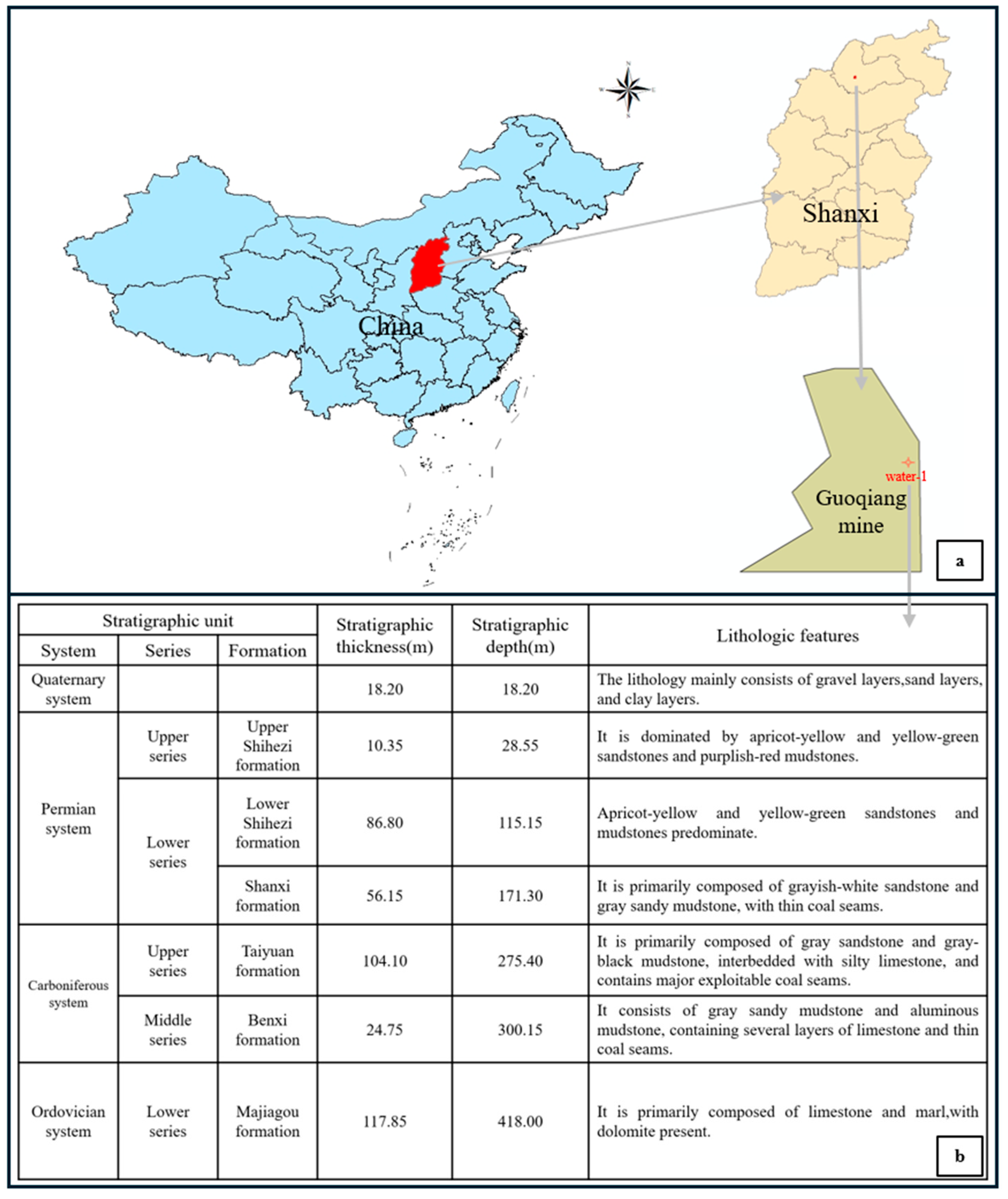
2. Overview of the Study Area

The Shanxi Guoqiang Mine is located in the Shentou Spring Area (Figure 1a), which has experienced the evolution of sedimentary environments from Carboniferous–Permian fluvial and swampy environments; to Permian–Jurassic transitional-phase environments where rivers, lakes, and deltas interacted with each other; to the arid terrestrial deposition of the Cretaceous period; and ultimately to the sedimentary environments of the Cenozoic impacts. This prolonged environmental evolution has undergone multiple episodes of marine–continental transitions, tectonic movements, and climatic changes, resulting in a highly complex stratigraphic structure within the mining area. Sediments from different geological periods have successively overlain one another, forming multi-layered and multi-facies lithological assemblages.

The stratigraphic sequence that developed within the well field, from top to bottom, is as follows: Quaternary (Q), Upper Permian Shihezi Formation (P₂s), Lower Permian Shihezi Formation (P₁x), Permian Shanxi Formation (P₁s), Carboniferous Taiyuan Formation (C₃t), Carboniferous Benxi Formation (C₂b), and Middle Ordovician Majiagou Formation (O₂) (Figure 1b).

The Quaternary rock layer is composed of sand, sub-sand, and gravel of varying degrees with a thickness of 18.20 m. The upper Shihezi Formation of the Permian system is mainly composed of yellow–green and dark purple sandy mudstone, with thin layers of yellow–green coarse sandstone, with a thickness of 10.35 m. The lower Shihezi Formation of the Permian system is mainly composed of gray–yellow and light yellow thick-layered medium–coarse sandstone, interbedded with blue–gray sandy mudstone and mudstone, with a layer of unstable coarse sandstone and gravelly sandstone at the bottom and a thickness of 86.60 m. The Shanxi Formation of the Permian System is one of the coal-bearing strata in the well field, and it is mainly composed of gray or grayish–white sandstone, grayish–black mudstone, sandy mudstone, and siltstone. The sandstone at the bottom is grayish–white fine sandstone and medium sandstone, which has locally transformed into siltstone. The Taiyuan Formation of the Carboniferous System is mainly composed of grayish–white or gray sandstone, grayish–black siltstone, sandy mudstone, mudstone, and six coal seams, and it is bounded by a layer of fine-grained sandstone at the bottom with the Benxi Formation. The Benxi Formation of the Carboniferous System is mainly composed of gray or grayish–white sandstone, sandy mudstone, and mudstone. The Shangmajiagou Formation of the Ordovician System is mainly blue–gray to dark gray limestone, dolomite, and dolomitic limestone, intercalated with grayish–yellow mudstone, muddy limestone, and calcareous mudstone, and it is in parallel unconformable contact with the underlying strata.

3. Basic Theory

3.1. LASSO Algorithm

The least absolute shrinkage and selection operator (LASSO) is a regularization technique for variable feature selection proposed by Tibshirani [12]. Its core principle is to use the sparsity of the L1 norm to achieve penalty optimization during regression. When the original data matrix has high dimensionality and redundant indicators, the LASSO algorithm can feature-screen the data, effectively reducing their dimensionality and reducing the modeling complexity [13]. Compared with other feature-screening methods, the LASSO algorithm introduces the L1 norm penalty term to compress some feature coefficients to 0, which can directly and effectively remove irrelevant parameters in high-dimensional, multivariate while-drilling parameters and improve the generalization ability of the model. In addition, the LASSO algorithm is easy to integrate with subsequent machine learning models, which is beneficial to subsequent data processing.

The fundamental idea of the LASSO algorithm is to minimize the residual sum of squares subject to the constraint that the sum of the absolute values of the regression coefficients is less than a certain constant. This leads to some coefficients being exactly zero, resulting in a more parsimonious model. The objective optimization problem of the algorithm can be expressed as follows [14]:

$$\widehat{\beta }={\arg }_{\beta }\min \left[{\displaystyle \sum _{i=1}^n(y_i-{\displaystyle \sum _{j=1}^m{x}_{i,j}{\beta }_j{)}^2+\lambda {\displaystyle \sum _{j=1}^m\left|{\beta }_j\right|}}}\right]$$

(1)

In this formula, $\widehat{\beta }$ is the estimated value of the regression coefficient; n is the number of samples; $y_i$ is the predicted value for the i-th sample; m is the number of input features samples; $x_{i,j}$ is the raw data of the sample; ${\beta }_j$ is the j-th regression coefficient; and $\lambda$ is the regularization parameter.

The LASSO algorithm consists of two components: the sum of squared prediction residuals and the L1 norm penalty term. $\lambda$ is the regularization strength parameter, which is used to regulate the complexity and sparsity of the model, and its size is obtained by cross-validation. LASSO introduces the L1 norm penalty term to compress the coefficients of some unimportant variables to 0. This mechanism enables the model to have the ability to select variables independently, thereby removing redundant information, preventing overfitting, and achieving more accurate parameter estimation.

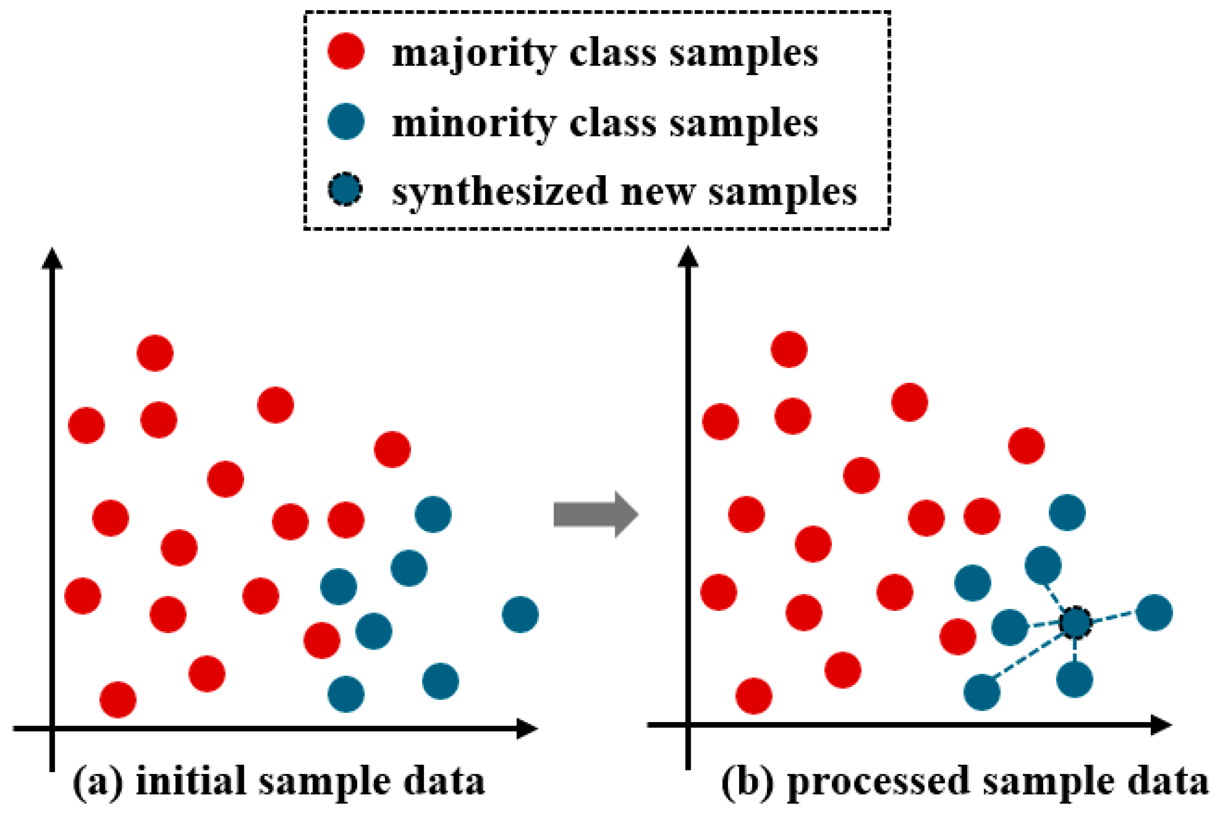
3.2. SMOTE Algorithm

Complex depositional environments can easily lead to uneven lithologic data samples, which can affect the identification accuracy. The SMOTE method, proposed by Chawla et al. [15], is a data preprocessing technique designed to address the problem of imbalanced data sets. Unlike random oversampling, which simply replicates minority class samples, SMOTE generates new synthetic samples by performing linear interpolation between existing minority samples. This approach effectively mitigates the overfitting issues commonly associated with random oversampling [16]. Compared with traditional undersampling, oversampling and other variant methods, SMOTE can improve the recognition ability of minority samples while maintaining model stability and overall performance. It is particularly suitable for the situation where rock samples are unevenly distributed in lithology identification.

The SMOTE algorithm utilizes the K-nearest neighbor algorithm to generate new samples: sample points X_i (i = 1, 2, 3, …) from a small number of classes of samples are sequentially selected as root samples for synthesizing new samples. Then, according to the sampling rate c, sample X_k is randomly selected from the K-nearest neighbor samples of the same category as X_i as an auxiliary sample, and this is repeated c times. According to Equation (2), linear interpolation is performed on the root sample and the auxiliary sample and, finally, a new sample point, X_new, is constructed [17].

$$X_{\mathrm{new}}=X_i+\mathrm{rand}(0,1)\left|X_i-X_k\right|,k=1,2,\dots ,c$$

(2)

The process of generating a new sample is shown in Figure 2 [18]. By synthesizing new features between minority class samples and their nearest neighbor samples to form new samples, the original data set can be processed into a class-balanced data set.

In this study, an adaptive K-domain setting method was used to protect the local structure of data with few categories and avoid overfitting. The number of nearest neighbors of the majority class was set to 8 to ensure that the SMOTE algorithm expanded the reference domain range when generating samples and enhanced the diversity and boundary representativeness of synthetic samples. A sample generation strategy focusing on the decision boundary was set to effectively avoid noise and excessively overlapping areas, further reducing the risks of synthesis failure and class overlap that may be caused in the generation of small sample and complex boundary geological data.

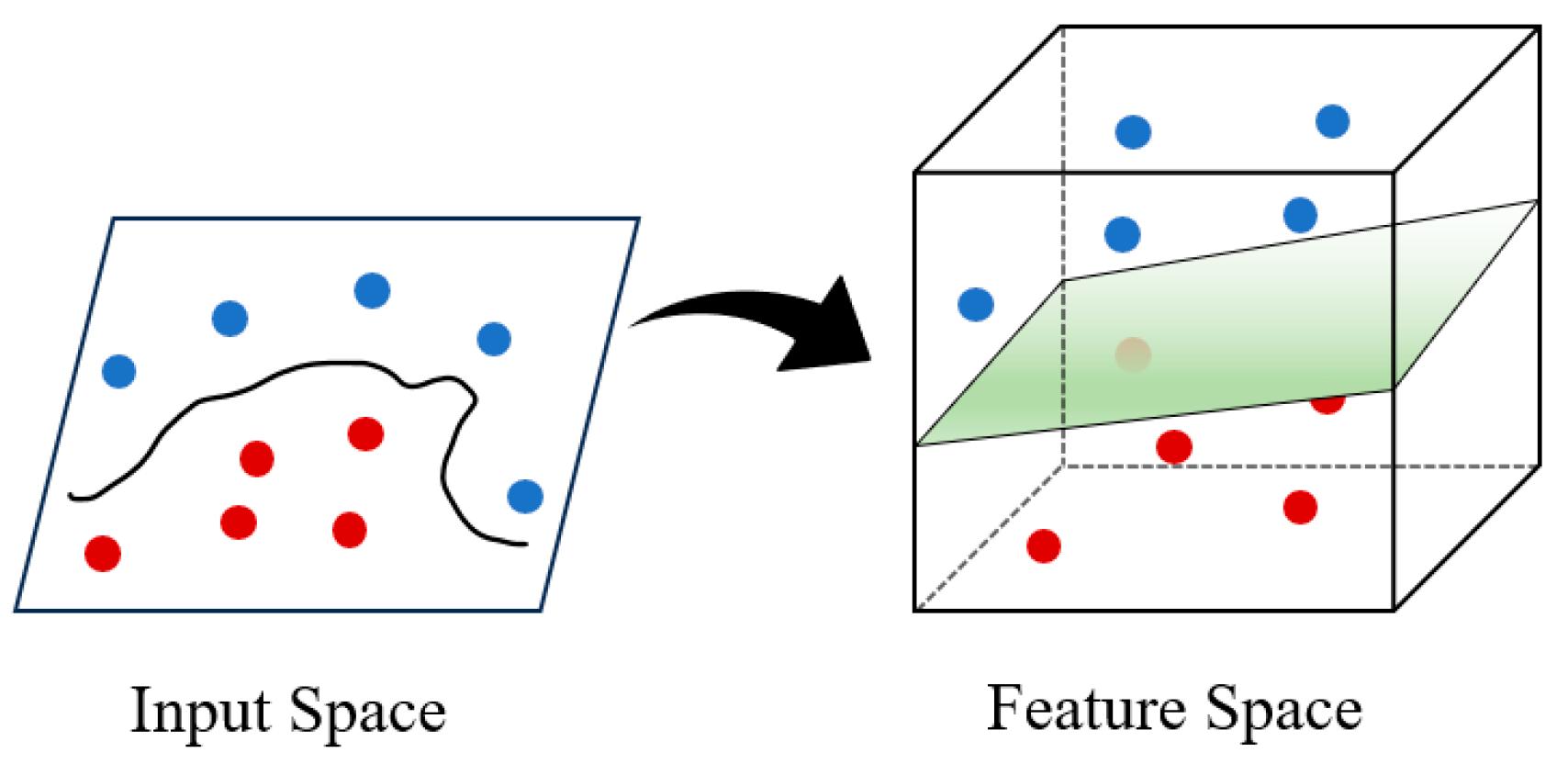
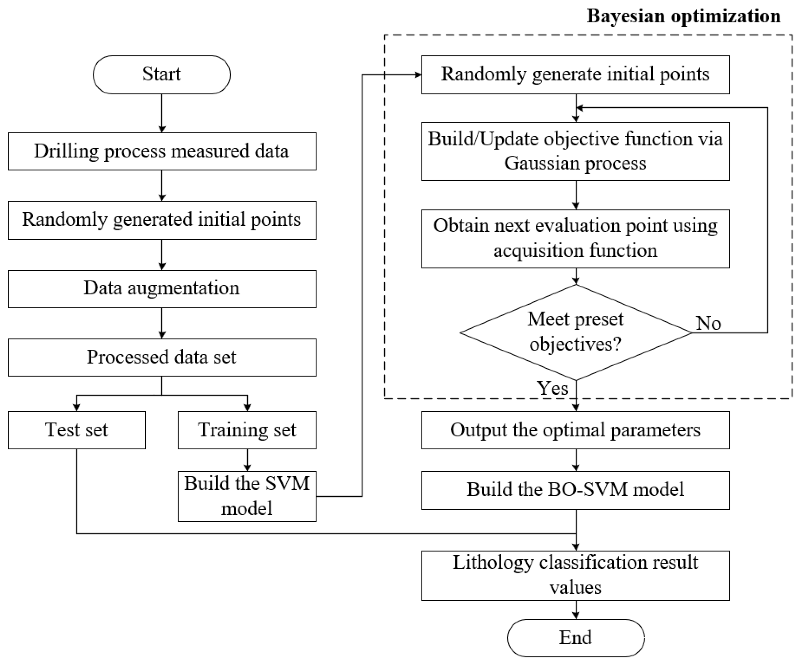
3.3. BO-SVM Algorithm

The principle of the SVM is to map data samples from a low-dimensional space to a higher-dimensional feature space where an optimal separating hyperplane is constructed. This hyperplane maximizes the margin between positive and negative samples in the training set, thereby achieving optimal classification (Figure 3) [19]. Compared with other classification methods, the SVM has unique advantages in solving nonlinear, small-sample problems and in high-dimensional pattern recognition (

Table 1. Comparison table of SVM and other common classification algorithms.

Algorithm	Advantages	Limitations	Comparison with SVM
Neural network	good fitting effect for big data	requires large number of samples, difficult to train	SVM model is more stable with smaller sample sizes
Random forest (RF)	good stability and high robustness	models are slow to train and difficult to interpret	SVM performs well on high-dimensional data [20]
K-nearest neighbors	simple model, fast training	more sensitive to outliers	SVM is more robust and has clearer decision boundaries [21]
XGBoost	simple model, good interpretability	inability to deal with nonlinearities	SVM can handle nonlinear problems

), but it also has the disadvantages of high model calculation complexity and sensitivity to parameters [20,21]. The penalty factor C and the kernel function hyperparameter γ are two important parameters in the SVM model. The penalty factor C controls the tolerance of the SVM model to training errors and affects the generalization performance of the model. The hyperparameter γ determines the distribution of data mapped to the new feature space and affects the speed of model training and prediction. However, the relationship between parameters C and γ and the model’s performance cannot be described by any expression. An optimal SVM model can only be obtained by traversing the discrete independent variables [22,23].

Bayesian optimization is an efficient systematic tuning algorithm that uses a Gaussian process to establish a probabilistic proxy model and continuously iteratively updates the proxy model to find the optimal parameter combination within the minimum number of iterations [24]. Compared with parameter adjustment methods such as grid search and random search, Bayesian optimization focuses on reducing the evaluation cost, requires fewer iterations, and is not prone to falling into local optimality. It has the characteristics of simple structure and efficient calculation. In lithology classification tasks, lithological features are often characterized by complex nonlinear relationships and indistinct class boundaries. The SVM model has good classification capabilities, but its performance is highly dependent on the type of kernel function and its parameter settings. The Bayesian optimization algorithm can accurately and efficiently find the optimal parameter combination by constructing a proxy model of the objective function, thereby improving the generalization performance of the SVM model and improving its recognition accuracy.

The process of Bayesian optimization of an SVM model is as follows [25]:

(1)

Set the parameter setting range to be optimized for the SVM model;

(2)

Input randomly generated initialization sample points into the Gaussian process and obtain the mean and standard deviation of the points to be determined based on the determined points;

(3)

Select the point with the best probability and calculate the corresponding true value of this point;

(4)

When the optimization condition is not met, the Gaussian model is updated, and the next optimal point with the best probability is selected and input into the modified Gaussian model. Iterations are repeated until the optimal parameter value of the support vector machine suitable for lithology identification is found.

In this study, in order to improve the effect and repeatability of lithology classification, we first adopted the TPE acquisition function, combined 10 random initial samplings with 40 directional samplings in the total number of 50 iterations to form a hybrid sampling strategy, and set the stopping standard to a fixed number of iterations to ensure that the optimization process is stable and controllable; secondly, the data were randomly shuffled to avoid the influence of the sample order in the original data on the division results; finally, a stratified 5-fold cross-validator was constructed to perform stratified grouping and cross-validation on the data set to ensure the convergence stability and result reliability of the BO-SVM model in lithology identification.

4. Model Building and Data Processing

4.1. Raw Data

In the process of drilling, the pressurized circulating mud provides power for the rotation of the drill bit, together with the thrust and torque of the drill pipe, to provide rock-breaking power [26]. Parameters such as the mud pressure, drilling speed, torque, slurry flow rate, and bottom hole pressure are all related to the crushing of the surrounding rock in the process of drilling, and there is also a certain connection between the depth of the drilled hole and different lithologies [27,28]. From previous research results and on-site measurements and recordings [29,30], six indices were comprehensively determined as drilling measurement parameters: the drilling speed, bottom hole pressure, mud pressure, slurry flow rate, torque, and hole depth. Through the drilling measurement system, changes in these parameters can be monitored and used to compose raw data sets; these data sets can then be used to effectively identify the rock hardness and other physical properties during the drilling process and provide valuable information for lithology identification during drilling.

In view of the complex cross-characteristics of the rock strata in the Guoqiang Coal Mine, the sampling frequency was increased for the layers where parameters changed greatly during drilling, and a total of 229 sets of data were produced. The 229 sets of data produced from the water-1 drill hole in the Guoqiang Coal Mine were used for this study. Part of the original data sample is shown in

Table 2. Sample table of raw data of drilling parameters.

Number	Figure						Lithology
	Drilling Speed /(m·h−1)	Bottom Hole Pressure/MPa	Mud Pressure /MPa	Slurry Flow Rate /(L·min−1)	Torque /(N·m)	Hole Depth /m
1	0.41	3.36	1.99	5.01	3830	3	loess
2	0.45	3.37	1.99	4.84	3922	6	loess
3	0.45	3.40	1.99	4.84	3238	9	loess
4	0.39	3.45	1.97	5.18	3342	12	loess
…	…	…	…	…	…	…	…
78	0.45	3.66	2.01	5.18	4628	113	sandy mudstone
79	0.45	3.67	2.02	5.18	4822	114	sandy mudstone
80	0.47	3.25	1.89	6.18	2899	115	mudstone
81	0.48	3.27	1.89	6.35	2788	116	mudstone
…	…	…	…	…	…	…	…
226	0.35	4.89	2.45	3.84	8905	406	limestone
227	0.35	4.87	2.45	3.84	8164	409	limestone
228	0.36	4.86	2.32	3.84	8263	412	limestone
229	0.37	4.86	2.32	3.67	8723	415	limestone

.

4.2. Model Building

In traditional lithology identification and classification models, the fuzzy features of the indicators and insufficient and unbalanced numbers of samples can lead to a poor model quality and low identification accuracy. Firstly, in order to solve the problem of weak correlations between indicators in traditional lithology identification, the LASSO algorithm is used herein to perform feature screening on the independent variables (six parameters), and the independent variables that contribute more to the prediction of the dependent variable (lithology) are screened out. The collinearity between the independent variables and the correlation between the independent variables and the dependent variables are analyzed to verify the algorithm results. Secondly, in order to solve the problem of low model generalization caused by small samples and sample imbalance in lithologically complex areas, the SMOTE algorithm is used to expand the data samples, increase the amounts of sample data in minority classes, keep the ratio of each lithological data set at 1:1, and reduce the dimension of the oversampled data set from a high-dimensional space to a low-dimensional space to observe whether there is obvious separation or overlap between different categories of data so as to verify the reliability of the generated data. Then, the Bayesian optimization algorithm is used to find the optimal parameter combination for SVM, and the processed sample data are input into the combined model to identify different lithologies. Finally, the combined model effect is evaluated by comparing it with different models and actual effects.

4.3. Effect Evaluation

The balanced data set was divided into 70% for training and 30% for testing the model. The XGBoost model, RF model, and single SVM model commonly used in lithology identification research were selected as the control group for the combined model to verify the actual effect of the oversampling algorithm and the recognition accuracy of the combined model.

The lithology recognition effects of each model were compared and analyzed by using core data and model evaluation indicators such as the accuracy (A_c), precision (P_r), recall (R_e), and F₁ score. The calculation formulas for these four evaluation indicators are shown in Equations (3)–(6):

$$A_{\mathrm{c}}={\displaystyle \frac{\mathrm{TP}+\mathrm{TN}}{\mathrm{TP}+\mathrm{FP}+\mathrm{FN}+\mathrm{TN}}}$$

(3)

$$P_{\mathrm{r}}={\displaystyle \frac{\mathrm{TP}}{\mathrm{TP}+\mathrm{FP}}}$$

(4)

$$R_{\mathrm{e}}={\displaystyle \frac{\mathrm{TP}}{\mathrm{TP}+\mathrm{FN}}}$$

(5)

$$F_1={\displaystyle \frac{2R_{\mathrm{e}}\cdot P_{\mathrm{r}}}{R_{\mathrm{e}}+P_{\mathrm{r}}}}$$

(6)

In these formulas, the meanings of TP, TN, FP, and FN are as shown in Figure 4.

The overall flow of the lithology identification analysis with drilling data is shown in Figure 5.

5. Results Analysis

5.1. Indicator Feature Screening

The LASSO algorithm was used to reduce the indicator size of the categorical data set; compress the coefficients of the unimportant variables to 0 via L1 regularization; screen out the independent variables that contribute more to the prediction of the lithology as the dependent variable to avoid estimation complexity and overfitting problems caused by too many indicator features; and test the results by examining the restricted cubic spline (RCS) R² values and variance inflation factor (VIF) coefficients. The results of indicator feature screening are shown in

Table 3. Indicator feature screening process operation results table.

	Drilling Speed	Bottom Hole Pressure	Mud Pressure	Slurry Flow Rate	Torque	Hole Depth
LASSO regression coefficients	−1.803	0	1.387	2.482	−0.119	0
R2 values	0.683	0.733	0.703	0.661	0.713	0.489
VIF coefficients	6.69	22.02	10.26	14.67	4.02	/
VIF coefficients of various indicators after removing the “bottom hole pressure”	6.53	/	7.56	6.31	4.02	/

.

The LASSO algorithm was used to gradually compress the coefficients of the independent variables, and four influencing factors related to the lithology were screened out: the drilling speed, mud pressure, slurry flow rate, and torque. The test results show the R² value for the hole depth indicator was less than 0.5 and significantly lower than those for the other variables, indicating that the hole depth had a slightly weaker explanatory power for the lithology identification model. After the hole depth was removed, a multicollinearity analysis among the variables was performed. The VIF value for the borehole bottom pressure indicator was significantly greater than those for the other variables, so it was removed. After this removal, the VIF analysis was performed again. The VIF coefficients of each remaining indicator were less than 10, indicating that there was no strong correlation among the independent variables. The test results were consistent with the results of the LASSO algorithm. The screened indicator variables could then be used for lithology identification and classification.

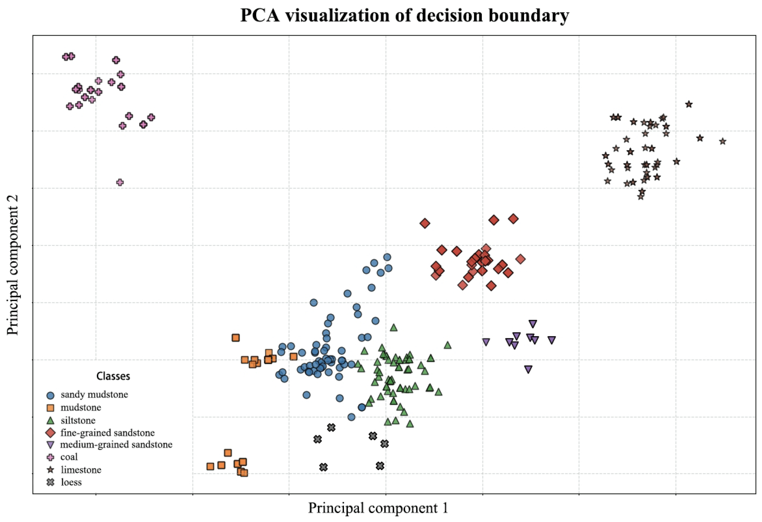
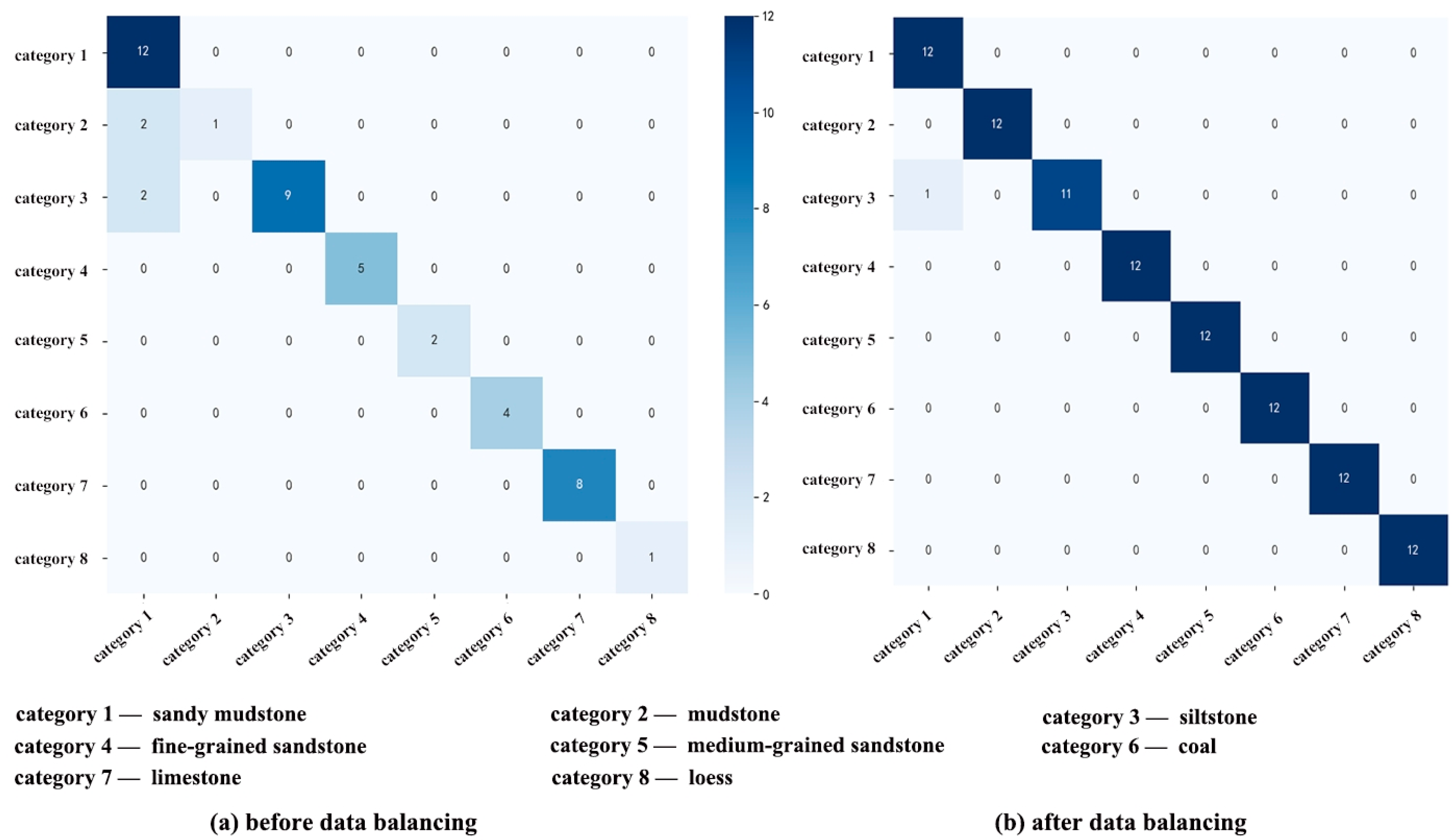
5.2. Sample Balance Processing

As can be seen from Table 2, in the original training data, the proportions of the sample categories were seriously unbalanced, and the numbers of “loess” and “medium-grained sandstone” samples were far lower than the numbers of other lithology samples. Good training results require a balanced data set: when directly applied to an unbalanced data set, classifiers tend to classify data into the majority category and ignore the minority category. In order to solve the problem of sample imbalance, the SMOTE algorithm was used to oversample the data set such that the number for each rock sample was kept at 60 groups; thus, the original 229 groups of data were expanded to 480 groups. This not only increased the number of samples but also made the sample categories more balanced.

In order to test whether there are abnormal situations such as the confusion of various sample characteristics or excessive dispersion of sample points after sample expansion, the expanded data set was reduced to a two-dimensional space using the principal component analysis (PCA) method. The results showed (Figure 6) that after the expansion, there was basically no overlapping area in the sample data, and the boundaries of each classification category were relatively clear, which was conducive to lithological classification. This indicated that the quality of the samples after balance processing was high.

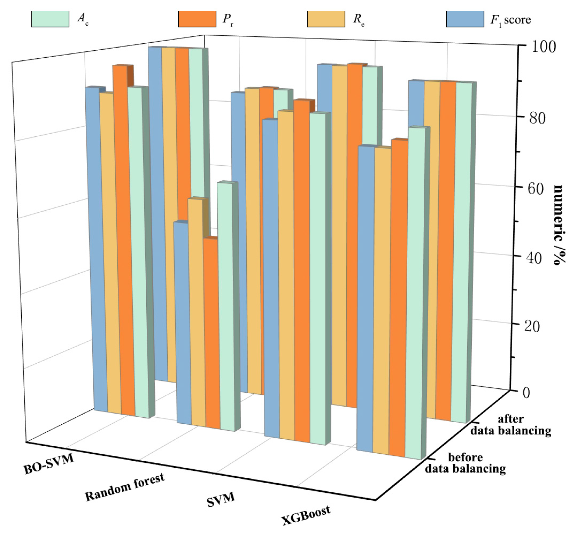
5.3. Results Comparison

Table 4. Comparison table of model evaluation index results before sample balancing.

Model	Evaluation Index
	Ac	Pr	Re	F1 Score
Random forest	0.674	0.522	0.625	0.558
XGBoost	0.848	0.815	0.793	0.794
SVM	0.870	0.901	0.871	0.847
BO-SVM	0.913	0.969	0.894	0.907

presents a comparison of the evaluation index operation results for the BO-SVM model and traditional machine learning models in lithology classification before sample balancing. Among them, the lithology classification accuracies of the RF, XGBoost, and SVM models did not exceed 90%. The RF model had the worst classification recognition accuracy, while the single SVM model had better classification accuracy than the other single machine learning models, indicating that it is more suitable for processing these kinds of unbalanced data samples. Through the Bayesian optimization algorithm, the key parameters of the SVM model were optimized, allowing it to surpass the other single machine learning models in all indicators in the lithology classification result evaluation. This shows that the SVM model after Bayesian optimization was maximized in terms of its model potential and achieved a good recognition effect when the number of samples was small. Compared with the single SVM model, its accuracy was improved by 4 percentage points, the effect was significant, and the actual running time was shorter. The analysis showed that the Bayesian optimization algorithm used a Gaussian process to establish the proxy model. A Gaussian process, as a probability distribution, corresponds to a global search. Through the acquisition function of the Gaussian process, a trade-off is made between exploring uncertain areas and focusing on areas known to have better target values. This allows the model to avoid the evaluation of many useless sampling points and accurately describe the distribution of the objective function, thereby efficiently finding the optimal parameter combination for the model and improving the model recognition effect.

Figure 7 presents a comparison of the evaluation index results for each model before and after sample balancing. Through the SMOTE oversampling algorithm, each model’s evaluation indicators greatly improved, and the accuracy of the single models basically increased to 90%. For the random forest model, with its poor original evaluation results, each evaluation indicator basically increased by 20 percentage points, which is a significant improvement. This shows that the SMOTE oversampling algorithm improved the actual discrimination effect of the models, especially for models with poor actual recognition effects. The improvement was obvious, which also indirectly shows that a good data set (more data and higher data quality) guarantees the operation of a machine learning model.

Furthermore, we plotted the confusion matrices of BO-SVM model recognition before and after sample equalization (Figure 8).

The matrices show that before sample balancing, the test set had a total of 46 groups of data, and the BO-SVM model correctly identified 42 groups of data with a recognition accuracy of 91.3%. For rock samples with sparse sample points (mudstone) and rock samples with more sample points (siltstone), the model identified them as sand and mudstone with similar properties, and both showed incorrect discrimination. After category balancing, there were 96 groups of test samples, and the BO-SVM model was able to correctly identify 95 groups of data. The recognition accuracy was increased from 91.3% to 99.0% with an error only in the identification of siltstone lithology. Obviously, the lithology identification effect of the proposed LASSO-SMOTE-BO-SVM hybrid model is better than that of the traditional machine learning models; the hybrid model effectively improves the accuracy of lithology identification and can be used in practical engineering applications.

6. Conclusions

This paper took the water-1 drilling data of the Guoqiang Coal Mine as the research object; used the LASSO algorithm to screen the characteristics of six main control indicators of lithology identification, the SMOTE oversampling algorithm to balance the samples, and the Bayesian optimization algorithm to optimize the parameters of the SVM model; and established a combined model for lithology identification research. The following conclusions were drawn:

• The four drilling parameters, namely drilling speed, mud pressure, slurry flow rate and torque, show high correlation with lithology identification, and there is no multicollinearity among the indicators, so they can be used as effective feature variables for the lithology identification classification task.
• The SMOTE oversampling algorithm is introduced to perform sample balancing on the training data. This expands the number of samples without affecting the sample quality and balances the sample categories. This effectively improves the classification performance of various models under imbalanced data conditions, especially for models that originally performed poorly. This method can be used as a solution to the sample imbalance problem.
• The Bayesian optimization algorithm is used to find the optimal parameters of the SVM model, and it is combined with the feature screening and sample balance algorithm to establish a combined model. Compared with the traditional lithology identification model, the results of this study are more in line with the actual engineering situation and can correctly identify 95 groups of data out of 96 test samples, indicating that the identification method after data optimization and model optimization has a good effect in lithology identification while drilling.
• With the rapid development of machine learning methods, deep learning models with higher accuracy and generalization performance such as convolutional neural networks and recurrent neural networks can be explored for application in lithology identification to further enhance the actual identification effect in engineering.

References

1. Asante-Okyere, S.; Shen, C.; Ziggah, Y.; Rulegeta, M.; Zhu, X. A Novel Hybrid Technique of Integrating Gradient-Boosted Machine and Clustering Algorithms for Lithology Classification. Nat. Resour. Res. 2020, 29, 2257–2273. [Google Scholar] [CrossRef]
2. Chen, L.; Ma, M.; Wang, H.; Liu, X.; Wu, M.; Hirota, K. Lithology Identification of Coal-Bearing Strata Based on Data-Driven Dual-Channel Relevance Networks in Coal Mine Roadway Drilling Process. Inf. Sci. 2025, 690, 121339. [Google Scholar] [CrossRef]
3. Yue, Z.; Yue, X.; Yang, R.; Wang, X.; Li, W.; Dai, S.; Li, Y. Research Progress of Lithology Identification Technology While Drilling. J. Min. Sci. Technol. 2022, 7, 389–402. [Google Scholar] [CrossRef]
4. Huang, J.; Ci, Y.; Liu, X. Research Status and Prospects of Intelligent Logging Lithology Identification. Meas. Sci. Technol. 2024, 36, 012010. [Google Scholar] [CrossRef]
5. Kahraman, S. Rotary and Percussive Drilling Prediction Using Regression Analysis. Int. J. Rock Mech. Min. Sci. 1999, 36, 981–989. [Google Scholar] [CrossRef]
6. Mostofi, M.; Rasouli, V.; Mawuli, E. An Estimation of Rock Strength Using a Drilling Performance Model: A Case Study in Blacktip Field, Australia. Rock Mech. Rock Eng. 2011, 44, 305–316. [Google Scholar] [CrossRef]
7. Shreedharan, S.; Hegde, C.; Sharma, S.; Vardhan, H. Acoustic Fingerprinting for Rock Identification During Drilling. Int. J. Miner. Eng. 2014, 5, 89–105. [Google Scholar] [CrossRef]
8. Kumar, B.; Vardhan, H.; Govindaraj, M. Prediction of Uniaxial Compressive Strength, Tensile Strength, and Porosity of Sedimentary Rocks Using Sound Level Produced During Rotary Drilling. Rock Mech. Rock Eng. 2011, 44, 613–620. [Google Scholar] [CrossRef]
9. Zhang, S.; Wang, B.; Ma, J. Deep Convolutional Auto-Encoder Based Lithologic Classification and Recognition. J. Signal Process. 2023, 39, 11–19. [Google Scholar] [CrossRef]
10. Wang, S.; Zhang, Z.; Chen, Q.; Zeng, W.; Bai, J.; Yin, S.; Chen, M. Lithology Identification Method Based on Deep Learning of Vibration and Sound Signals. Sci. Technol. Eng. 2023, 23, 2759–2767. [Google Scholar] [CrossRef]
11. Guan, Y.; Wang, Q.; Feng, J.; Yang, Q.; Shi, L. Comprehensive Lithology Recognition of Altered Igneous Reservoirs Based on Machine Learning for Wireline and Cutting Logs in Huizhou Depression, Pearl River Mouth Basin, Northern South China Sea. J. Jilin Univ. (Earth Sci. Ed.) 2024, 54, 345–358. [Google Scholar] [CrossRef]
12. Tibshirani, R. Regression Shrinkage and Selection Via the Lasso. J. R. Stat. Soc. B Methodol. 1996, 58, 267–288. [Google Scholar] [CrossRef]
13. Zhong, H.; Hu, H.; Hou, N.; Fan, Z. Study on Abnormal Pattern Detection Method for In-Service Bridge Based on Lasso Regression. Appl. Sci. 2024, 14, 2829. [Google Scholar] [CrossRef]
14. Friedman, J.; Hastie, T.; Tibshirani, R. Regularization Paths for Generalized Linear Models via Coordinate Descent. J. Stat. Softw. 2010, 33, 1–22. [Google Scholar] [CrossRef]
15. Chawla, N.; Bowyer, K.; Hall, L.; Kegelmeyer, W. SMOTE: Synthetic Minority Over-Sampling Technique. J. Artif. Intell. Res. 2002, 16, 321–357. [Google Scholar] [CrossRef]
16. Shi, H.; Chen, Y.; Chen, X. Summary of Research on SMOTE Oversampling and Its Improved Algorithms. CAAI Trans. Intell. Syst. 2019, 14, 1073–1083. [Google Scholar] [CrossRef]
17. Sayegh, H.; Dong, W.; Al-madani, A. Enhanced Intrusion Detection with LSTM-Based Model, Feature Selection, and SMOTE for Imbalanced Data. Appl. Sci. 2024, 14, 479. [Google Scholar] [CrossRef]
18. Huang, A.; Cai, W.; Wei, X.; Li, Y.; Duan, G.; Liu, D. Lithology Identification of Volcanic Rock Logging Based on Improved Random Forest. Sci. Technol. Eng. 2023, 23, 3696–3704. [Google Scholar] [CrossRef]
19. Mou, D.; Wang, Z.; Huang, Y.; Xu, S.; Zhou, D. Lithology Identification of Volcanic Rocks Based on SVM Logging Data: A Case Study of the Eastern Depression of Liaohe Basin. Chin. J. Geophys. 2015, 58, 1785–1793. [Google Scholar] [CrossRef]
20. Huang, F.; Wu, D.; Chang, Z.; Chen, Q.; Tao, J.; Jiang, S.; Zhou, C. Landslide Susceptibility Pattern and Potential Landslide Identification under Sample Deficiency: A Susceptibility–InSAR Multi-Source Information Method. J. Rock Mech. Eng. 2025, 44, 584–601. [Google Scholar] [CrossRef]
21. Weng, Y.; Zhang, W.; Gao, L. Risk Assessment of Rainfall-Induced Landslides Based on SHALSTAB-SVM Model: A Case Study of Daguan County, Yunnan Province. Sediment. Geol. Tethyan Geol. 2024, 44, 523–533. [Google Scholar] [CrossRef]
22. Mukhamediev, R.; Kuchin, Y.; Yunicheva, N.; Kalpeyeva, Z.; Muhamedijeva, E.; Gopejenko, V.; Rystygulov, P. Classification of Logging Data Using Machine Learning Algorithms. Appl. Sci. 2024, 14, 7779. [Google Scholar] [CrossRef]
23. Zhang, X. Evaluation of Landslide Susceptibility Based on Bayesian Algorithm Optimized Machine Learning Model—Example of Liliu Coal Mining Area. Master’s Thesis, Taiyuan University of Technology, Taiyuan, China, 2023. [Google Scholar] [CrossRef]
24. Feng, R.; Chen, Z.; Yi, S. Study on Maize Variety Identification Based on Bayesian Optimization of SVM. Spectrosc. Spectr. Anal. 2022, 42, 1698–1703. [Google Scholar] [CrossRef]
25. Yang, M.; Tian, H. Short-Term Wind Power Forecasting Based on Bayesian Optimized XGBoost. Electron. Devices 2024, 47, 1389–1395. [Google Scholar] [CrossRef]
26. Cheng, Y.; Wang, C.; Liu, X.; Liu, J.; Chen, S.; Huang, S. Application of Machine Learning-Based Lithology Identification Analysis for Tunnel Geological Survey. Tunnel Constr. 2023, 43, 1549. [Google Scholar] [CrossRef]
27. Yang, W.; Yue, Z.; Tham, L. Automatic Monitoring of Inserting or Retrieving SPT Sampler in Drillhole. Geotech. Test. J. 2012, 35, 103450. [Google Scholar] [CrossRef]
28. Song, L.; Li, N.; Li, Q. Study on the Intrinsic Relationship between Rotary Penetration Parameters and Mechanical Parameters of Soft Rock. Rock Soil Mech. Eng. J. 2011, 30, 1274–1282. [Google Scholar]
29. Yue, Z. Improvement and Enhancement of Engineering Rock Mass Quality Evaluation Method Based on Drilling Process Monitoring (DPM). Rock Soil Mech. Eng. J. 2014, 33, 1977–1996. [Google Scholar] [CrossRef]
30. Chen, J.; Yue, Z.Q. Hole Collapse Detection Based on Full Drill Analysis of DPM System. Eng. Geotech. Investig. 2010, 38, 26–31. [Google Scholar]
Figure 1. Location map of the study area (a) and histogram of the water-1 boreholes examined in this study (b).
Processes 13 02038 g001
Figure 2. Schematic diagram of sample data processed using SMOTE algorithm.
Processes 13 02038 g002
Figure 3. A schematic diagram of the principle of the support vector machine algorithm.
Processes 13 02038 g003
Figure 4. Binary confusion matrix (taking sandy mudstone as an example).
Processes 13 02038 g004
Figure 5. Bayesian optimization SVM flow chart.
Processes 13 02038 g005
Figure 6. Feature space distribution diagram after sample balancing.
Processes 13 02038 g006
Figure 7. Comparison of evaluation index results for each model before and after sample balancing.
Processes 13 02038 g007
Figure 8. Confusion matrix diagram of rock sample data before and after sample balancing.
Processes 13 02038 g008