Abstract
In order to study the problem of obvious wall thinning in the wellbore caused by proppant backflow and sand production under throttling conditions in tight gas wells. Based on the gas-phase control equation, particle motion equation, and erosion model, the wellbore erosion model is established. The distribution law of pressure, temperature, and velocity trace fields under throttling conditions is analyzed, and the influences of different throttling pressures, particle diameters, and particle mass flows on wellbore erosion are analyzed. The flow field at the nozzle changes drastically, and there is an obvious pressure drop, temperature drop, and velocity rise. When the surrounding gas is completely mixed, the physical quantity gradually stabilizes. The erosion shape of the wellbore outlet wall has a point-like distribution. The closer to the throttle valve outlet, the more intense the erosion point distribution is. Increasing the inlet pressure and particle mass flow rate will increase the maximum erosion rate, and increasing the particle diameter will reduce the maximum erosion rate. The particle mass flow rate has the greatest impact on the maximum erosion rate, followed by the particle diameter. The erosion trend was predicted using multiple regression model fitting of the linear interaction term. The research results can provide a reference for the application of downhole throttling technology and wellbore integrity in tight gas exploitation.
1. Introduction
Tight gas is an important unconventional oil and gas resource [1,2,3]. Tight gas is widely developed in the Sichuan Basin of China. The predicted geological resources are 6.9 trillion cubic meters, and the development potential is great [4,5]. Tight gas reservoirs are characterized by low porosity and ultra-low permeability [6,7,8,9]. The gas field is buried deeper, the reservoir pressure is higher, and the gas–water relationship is complex, which leads to higher wellhead pressure of gas wells [10,11]. Downhole throttling technology can reduce the wellhead pressure of gas wells, make full use of the formation energy to heat the raw gas, reduce the risk of wellbore effusion [12,13,14], simplify the surface throttling and heating process, and greatly reduce the safety risks of production and operation and the cost of station construction [15,16]. There are different degrees of proppant backflow in each well, and there is an obvious wall thinning problem in the wellbore [17,18,19]. Sand production in gas wells may cause erosion of the wellbore, making the integrity of the wellbore worse and requiring higher maintenance technology and costs. The gas velocity after throttling is higher, which may pose a greater threat to the wellbore [20]. Therefore, the effect of sand production on wellbore erosion under throttling conditions in tight gas wells needs to be further studied.
At present, scholars mainly use the CFD method to simulate the flow field under working conditions in natural gas wells. Zheng Jie et al. [21] comprehensively established a multi-physical field and multi-phase coupling throttling model with higher calculation accuracy than the simulation results of PIPESIM. They analyzed the temperature field, pressure field, and velocity field under the conditions of downhole throttling technology. Faqing Wang et al. [22,23] calculated the daily gas production after downhole throttling and found that a lower gas flow rate can enhance the Joule–Thomson (JT) cooling effect of downhole throttling. G Y Huo et al. [24] used ANSYS finite element analysis software to analyze the mechanical structure of the downhole intelligent throttle valve and the fluid field of the key parts of the throttle valve and determined the feasibility of throttle valve design. Jia Lin Tian et al. [25] studied the flow field changes under different nozzle diameters under the conditions of a well depth of 2000 m using the CFD method and found that downhole throttling had an obvious influence on the pressure, velocity, and temperature fields. When the diameter of the throttling nozzle increased, the maximum velocity of the outlet flow increased and the minimum outlet pressure decreased. Xing Xuesong et al. [26] used Fluent to simulate the supercritical flow of an adjustable multi-hole throttling device. It was found that the velocity distribution between the channels of the downhole multi-hole throttling device was not uniform. The speed increased rapidly and then decreased at the exit, while the pressure decreased briefly and then increased slightly. At the same time, it was found that the pressure drop of the porous throttling device was inversely proportional to the number of holes. Tang Yang et al. [17] proposed a multi-stage throttling device that could effectively control the gas flow rate and pressure. The internal flow field of the multi-stage throttling device was simulated. It was found that the multi-stage throttling structure could accurately control the throttling cooling and mass flow range by adjusting the opening of the valve core. Changjun Li et al. [27,28] considered the anti-condensation phenomenon in the throttling time of natural gas, discussed the influence of inlet pressure and inlet temperature on the spontaneous condensation process in the throttle valve, proposed the empirical correction coefficients α and β of droplet nucleation, and analyzed the erosion effect of natural gas on the valve. Ma Huiyun et al. [29] used ANSYS Fluent to simulate the gas flow state and the trajectory of sand particles at the fixed downhole throttle valve. It was found that the flow field at the inlet and outlet of the throttle pipe changed the most, and the most serious erosion was obtained at the throttle valve. It can be seen that many scholars believe that the inlet and outlet flow fields in the throttling area change the most, and the throttling valve is seriously eroded.
Many scholars have carried out a lot of modeling research on wellbore erosion caused by sand production and proppant backflow in gas wells. Stavropoulou et al. [30] first used the Galerkin finite element method to numerically solve the erosion equation to analyze the wellbore erosion law. It was found that the erosion near the wellbore was the most serious, and erosion would cause changes in the mechanical behavior of the pipe. Hu Xiaodong et al. [31] simulated the particle migration of single-cluster and double-cluster horizontal well perforation fracturing and found that perforation erosion would affect the transportation and distribution of proppant in the horizontal wellbore. Subsequently, Zeng Dezhi et al. [32,33] established a perforation diameter prediction model for large-scale sand and gravel during fracturing. It was found that the solid particles had obvious wear or fragmentation, and the high-viscosity liquid had strong sand carrying capacity. The increase in sand production would lead to a larger erosion area and erosion rate. Asad and Abdul [34] established a reservoir-wellbore flow model to calculate high-speed solid particle flow, and the WEPP model was used to calculate sand erosion. It was found that erosion was more obvious in the early stage. As the simulation time increased, the wellbore surface became smoother and the erosion rate decreased. Majid Fetrat et al. [35] used the finite element method combined with the sand production criterion to study sand production in the hydraulic-mechanical wellbore. It was found that the plastic shear strain and erosion rate criterion could accurately predict the sand production and erosion rate of the wellbore. Binqi Zhang et al. [36] used the CFD-DPM method to conduct simulation research and proposed an erosion model suitable for coiled tubing under gas–solid two-phase flow conditions. Considering the mechanical behavior of porous media and the influence of sand production, Xiaorong Li et al. [37] proposed a finite element-based model to capture the eroded surface using cell adaptive technology. The model simulated the stress distribution and erosion rate around the wellbore during drilling, completion, and production stages. It was found that the maximum and minimum stress distribution areas were more prone to erosion. Although there are existing studies on throttle valve erosion and wellbore erosion for reference, compared with throttle valves, wellbore erosion is more concealed and harder to detect in a timely manner, which urgently requires attention from the industry.
This study constructs a wellbore erosion model by coupling the gas-phase control equation, particle motion equation, and erosion model based on the CFD-DPM method, and it conducts simulation analyses on the downhole throttling flow field. The study clarifies the distribution characteristics of the pressure field, temperature field, flow velocity field, and density field under throttling conditions and systematically explores the influence laws of different throttling pressure differences, particle diameters, and particle mass flow rates on wellbore erosion, which can provide technical support for the safe exploitation of tight gas.
2. High-Pressure Downhole Throttle Valve Structure
2.1. Throttle Valve Structure
In order to study the fluid distribution characteristics and wellbore erosion under downhole throttling conditions in the process of high-pressure tight gas exploitation, the fixed downhole choke HWS47 is modeled as the research object (Figure 1a). On the premise of meshing, the internal flow field of the valve is taken out and simplified reasonably, as shown in Figure 1b. The whole model includes two parts: the wellbore and the throttle valve. The lower part is the wellbore inlet, with a length of 50 mm, the upper part is the wellbore outlet, with a length of 1000 mm, and the inner diameter of the wellbore is 62 mm. The downhole throttle valve is composed of a throttle nozzle and a throttle cylinder. The length of the throttle nozzle is 20 mm, with an inner diameter of 8 mm, and the length of the throttle working cylinder is 280 mm, with an inner diameter of 46 mm.
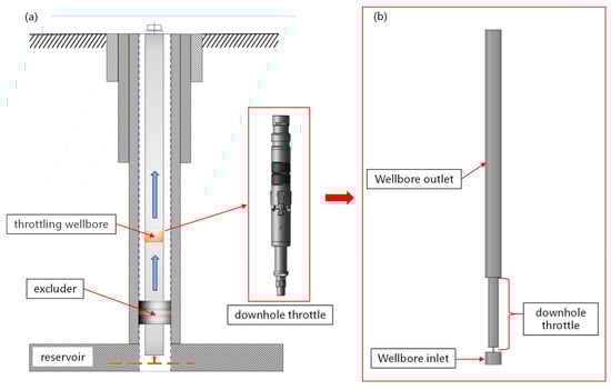
Figure 1.
Structure diagram of fixed downhole choke. (a) HWS47 fixed downhole choke structure; (b) fluid domain at the restrictor.
2.2. Mesh Subdivision
The mesh generation was performed using Fluent Meshing software (Figure 2). A poly-hexcore mesh was employed throughout the domain, with a base element size of 2 mm. Given the significant gradients in pressure, temperature, and velocity near the choke nozzle, local mesh refinement was applied to this region at a refinement ratio of 3:1. Additionally, five boundary layer elements were added to the fluid domain, with the first layer height set to 0.1 mm and a growth rate of 1.1, ensuring a y+ value range of approximately 30.
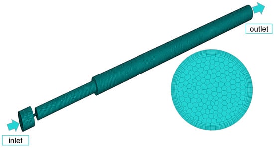
Figure 2.
Cell division.
2.3. Mesh-Free Verification
In order to ensure the accuracy of the calculation results, the maximum calculated flow rate in the throttle valve was used as the cell independence verification index, and six cells with different densities were divided. The numbers of cells were 265,980, 315,988, 409,602, 609,240, 803,789, and 1,027,454. The inlet pressure was 100 MPa, the outlet pressure was 30 MPa, the particle mass flow rate was 1 × 10⁻³ kg/s, the particle inlet velocity was 2 m/s, and the particle size was 50 μm. The maximum flow velocity in the throttle valve under 6 cells was calculated, as shown in Figure 3. When the number of cells was 609,240, the flow velocity was 503.641, and the relative error of the maximum flow velocity in the throttle valve was less than 0.01% when the numbers of cells were 803,789 and 1,027,454. It can be considered that the number of cells had no effect on the calculation results. In order to ensure the calculation accuracy and calculation efficiency, a cell number of 609,240 was finally selected for subsequent calculations.
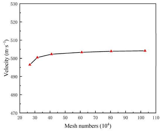
Figure 3.
Verification of cell independence.
2.4. Numerical Solution Method
Due to the high inlet pressure of 100 MPa, adopting ideal gas in the calculation of natural gas density is difficult. The density was calculated using the real gas Soave–Redlich–Kwong equation of state. The density of solid particles was fixed at 1600 kg/m3. Since achieving non-hypersonic flow (Ma ≥ 2) is difficult in the throttle valve, the pressure basis was selected to solve the problem in order to ensure the stability of the calculation results. The turbulence model of fluid flow was the realizable k–ε model, which is suitable for high Reynolds number flow. The extensible wall function was selected to simplify the near-wall treatment. The discrete phase model was selected considering the energy transfer and viscous heating particle motion equation. The erosion model was the generic erosion model, and the steady-state coupled method was selected to solve the problem. The inlet and outlet were set as the pressure inlet and pressure outlet, respectively, and the initial condition was mixed initialization. The throttle valve and wellbore wall were adiabatic non-slip walls. In order to study the wellbore erosion behavior, the throttle wall was set not to erode, and only the wellbore wall was used to calculate the erosion rate.
3. Mathematical Model
3.1. Gas-Phase Control Equation
The tight gas in the fluid domain should satisfy the continuity equation, momentum equation, and energy equation, as shown in Equations (1)–(3):
where is the density, kg/m3; is the fluid velocity, m/s; is time; is pressure, Pa; is the stress tensor of viscous force; is the unit mass force; is the specific internal energy, j/kg; is the thermal conductivity, W/(m·K); is temperature, K; is a viscous dissipation function; and is the intensity of the internal heat source.
3.2. Particle-Phase Motion Equation
The trajectory and force of quartz sand particles are controlled by the particle phase motion equation. The main forces include mass force, fluid drag force, gravity, buoyancy, additional mass force, etc., as shown in Equations (4)–(6). There are also many forces in particle motion, such as Basset force, Magnus force, and Saffman force. The Basset force is an instantaneous flow resistance, which is related to the stability of the fluid. Since there is no obvious acceleration or deceleration process of the particles in the wellbore, the force is ignored. Magnus and Saffman forces are only meaningful in specific cases, such as high-speed rotation of particles and small particle size, so they can be ignored in force analysis.
where is the particle mass, kg; is the particle velocity; is the dense gas velocity; is the drag force; is gravity; is the buoyancy; is the additional mass force; is the drag coefficient; is the particle projection area; is the fluid density; and is the particle diameter.
3.3. Turbulent Flow Model
Numerous studies have conducted comparative analyses of various turbulence models, and the results indicate that under high Reynolds number conditions, the differences in calculation results among the standard k–ε model, RNG k–ε model, and realizable k–ε model are negligible [38]. The realizable k– model suitable for high Reynolds number flow was selected. The model is based on two transport equations: the turbulent energy equation (K) and dissipation equation (), as shown in Equations (7) and (8):
where is the turbulence energy; is the turbulent viscosity, Pa·s;
is the turbulent kinetic energy dissipation rate; and
and are constant parameters.
3.4. State Equation
In the high pressure environment of the wellbore, natural gas cannot be regarded as a simple ideal gas calculation. According to the research by Shoghl et al. [39], the SRK equation of state (SRK EOS) is superior to RK EOS and PR EOS in terms of the accuracy of predicting the physical parameters of natural gas in throttle valves. Therefore, the cubic SRK equation of state was selected for relevant calculations in this study. The Soave–Redlich–Kwong Equations (9)–(11) commonly used in natural gas were introduced, which can better predict gas density. The throttling effect has the phenomenon of temperature reduction, and the Sutherland formula was introduced to calculate the gas viscosity.
where is the general gas constant; and are parameters related to material properties; is the critical temperature, is the critical pressure; is the eccentricity factor; is the gas viscosity, kg/(m s); and is the Sutherland constant.
3.5. Erosion Model
The generic erosion model comprehensively incorporates key parameters such as fluid velocity, particle characteristics (particle size, density, and concentration), and material properties (hardness). In their study on wellbore erosion behavior in gas storage reservoirs, Yanxing Yang et al. [40] compared experimental data with the prediction results of various erosion models (including the generic model, Finnie model, McLaury model, Oka model, and DNV model) and found that the prediction results of the generic erosion model showed the highest consistency with the experimental data. The generic erosion model suitable for pipeline and valve erosion was selected, as shown in Equation (13):
where
is the erosion rate, kg/(m2·s);
,
,
, and
are empirical coefficients related to particle type; and is the impact angle of the particles.
4. Results and Discussion
4.1. Throttling Flow Field Analysis
In order to understand the pressure drop, temperature drop, and velocity change of the flow field in the internal area of the throttle valve, the flow field distribution under the conditions of an inlet pressure of 100 MPa and temperature of 350 K was simulated. The pressure, temperature, and velocity contours are shown in Figure 4, Figure 5, and Figure 6, respectively. It can be seen from the figures that there is an obvious pressure drop and temperature drop after the throttling of tight gas. Before throttling, the pressure in the wellbore does not change significantly. Due to the sudden reduction in the inlet area of the throttling nozzle, the flow velocity channel suddenly narrows, and the pressure energy is transformed into kinetic energy, resulting in the internal flow field from high pressure to low pressure. The pressure has a certain recovery in the throttling nozzle, and the pressure gradually stabilizes after entering the throttling working cylinder. The conversion of pressure energy into kinetic energy leads to an increase in gas flow rate. Not far from the throttling outlet, the high-speed gas begins to decrease with mixing with the surrounding gas. After throttling, the pressure decreases, the gas expands, and the intermolecular potential energy increases, resulting in a decrease in temperature. When the high-speed low-temperature gas is completely mixed with the surrounding gas, the pressure, temperature, and speed gradually stabilize. The temperature drop area in the flow field is basically consistent with the high-speed area in the velocity cloud.
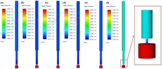
Figure 4.
Pressure cloud diagram of throttle valve area. (a) 50 MPa; (b) 60 MPa; (c) 70 MPa; (d) 80 MPa; (e) 90 MPa; (f) 100 MPa.
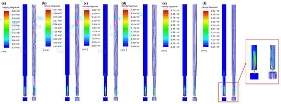
Figure 5.
Velocity and trace cloud map of the internal region of the throttle valve. (a) 50 MPa; (b) 60 MPa; (c) 70 MPa; (d) 80 MPa; (e) 90 MPa; (f) 100 MPa.
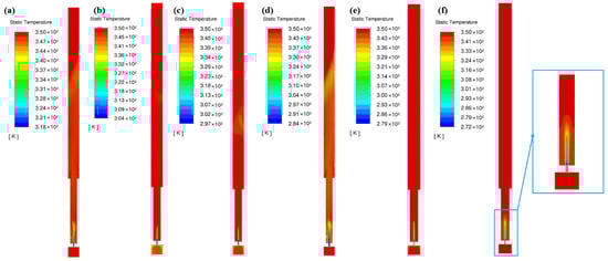
Figure 6.
Temperature cloud diagram of internal area of throttle valve. (a) 50 MPa; (b) 60 MPa; (c) 70 MPa; (d) 80 MPa; (e) 90 MPa; (f) 100 MPa.
In order to clarify the characteristics of pressure, temperature, and velocity changes, the pressure, temperature, and velocity changes on the central axis of the model were extracted, as shown in Figure 7, Figure 8 and Figure 9, respectively. After the high-pressure tight gas enters the throttle nozzle, the high pressure instantaneously drops to the lowest pressure and then stabilizes in the throttle working cylinder and the wellbore outlet. The higher the inlet pressure, the greater the throttling pressure drop in the throttle valve, and the higher the stable pressure. The pressure range after the 50 MPa–100 MPa inlet pressure throttling is 29.59 MPa to 32.07 MPa.
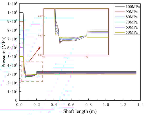
Figure 7.
Axis pressure change.

Figure 8.
Axis temperature change.
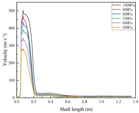
Figure 9.
Axial velocity change.
It can be seen from Figure 8 that the higher the inlet pressure, the greater the throttling temperature drop in the throttle valve, but after the high-speed low-temperature gas of the throttling working cylinder is completely mixed with the surrounding gas, the temperature is about 350 K. The trend of temperature drop in this study is highly consistent with the research results of Xuesong Xing [26] and Yang Tang [17], which serves as strong evidence for the accuracy of the established model.
It can be seen from Figure 9 that the inlet flow rate of the tight gas is 2–4 m/s, and the gas flow rate rises rapidly in the throttling nozzle to reach the highest flow rate. The flow rate decreases in the throttling working cylinder, but the flow rate after entering the wellbore is still higher than the inlet velocity of the wellbore. The gas flow rate in the wellbore easily causes erosion of the wellbore. The higher the inlet pressure, the higher the flow rate in the throttling nozzle and the wellbore.
4.2. Analysis of Influencing Factors of Wellbore Erosion
4.2.1. Effect of Inlet Pressure on Wellbore Erosion
The maximum erosion rate nephogram of the wellbore outlet section was simulated under the conditions of a particle mass flow rate of 1 × 10⁻³ kg/s, particle size of 50 μm, and inlet pressures of 50 MPa, 60 MPa, 70 MPa, 80 MPa, 90 MPa, and 100 MPa (Figure 10). It can be seen that the erosion shape of the wellbore outlet wall has a point-like distribution. The closer to the throttle valve outlet, the more intense the erosion point distribution is. The maximum wellbore erosion rate under different inlet pressures was extracted (Figure 11). As the inlet pressure increases, the maximum erosion rate increases rapidly. When the inlet pressure increases from 50 MPa to 100 MPa, the maximum erosion rate increases from 2.76 × 10⁻⁷ [kg/(m2 s)] to 3.64 × 10⁻⁷ [kg/(m2 s)], an increase of 31.88%. This is because the main source of particle kinetic energy is the conversion of gas pressure energy. After the greater inlet pressure throttling pressure drop, the gas in the wellbore carries the particle at a higher speed, and the wellbore erosion is more serious.
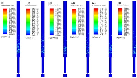
Figure 10.
Shaft erosion cloud diagram under different pressure inlets. (a) 50 MPa; (b) 60 MPa; (c) 70 MPa; (d) 80 MPa; (e) 90 MPa; (f) 100 MPa.
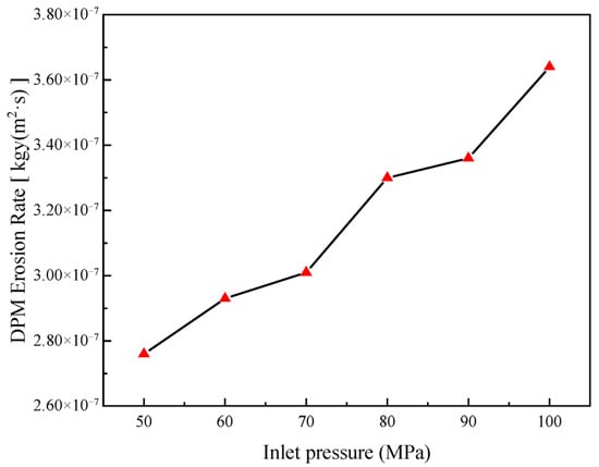
Figure 11.
Variation law of maximum erosion rate at different pressure inlets.
4.2.2. Effect of Particle Diameter on Wellbore Erosion
Using the above model to simulate the conditions of a particle mass flow rate of 1 × 10⁻³ kg/s, an inlet pressure of 100 MPa, and particle diameters of 50 μm, 70 μm, 90 μm, 110 μm, and 130 μm, and the maximum erosion rate at the wellbore outlet was simulated (Figure 12). It can be seen that the erosion shape of the wellbore outlet wall has a point-like distribution. The larger the particle diameter, the sparser the erosion point distribution, and the erosion point gradually moves up. The maximum wellbore erosion rate under different particle diameters was extracted (Figure 13). The maximum erosion rate of the wellbore outlet wall gradually decreases and then tends to be gentle. When the particle diameter increases from 50 μm to 130 μm, the maximum erosion rate decreases from 3.64 × 10⁻⁷ [kg/(m2 s)] to 1.80 × 10⁻⁷ [kg/(m2 s)], a decrease of 50.55%. This is due to the fact that the increase in particle diameter will reduce the number of particles and reduce the maximum erosion rate when the particle mass flow rate is fixed. When the diameter of a single particle increases to the critical particle size, the erosion effect of a single particle collision will be significantly aggravated, making up for the decrease in the number of particles.
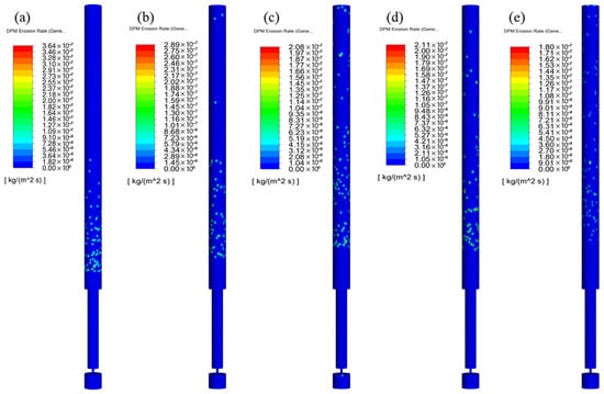
Figure 12.
Shaft erosion cloud diagram under different particle diameters. (a) 50 μm; (b) 70 μm; (c) 90 μm; (d) 110 μm; (e) 130 μm.
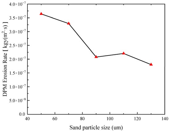
Figure 13.
Variation in maximum erosion rate with different particle diameters.
4.2.3. Effect of Particle Mass Flow Rate on Wellbore Erosion
The above model was used to simulate an inlet pressure of 100 MPa, a particle size of 50 μm, a particle mass flow rate of 1 × 10⁻³ kg/s, 2 × 10⁻³ kg/s, 3 × 10⁻³ kg/s, 4 × 10⁻³ kg/s, and 5 × 10⁻³ kg/s, the maximum erosion rate at the wellbore outlet (Figure 14), and the maximum wellbore erosion rate under different particle diameters (Figure 15). It can be seen that with the increase in mass flow rate, the maximum erosion rate of the wellbore outlet wall gradually increases. When the particle mass flow rate increases from 1 × 10⁻³ kg/s to 5 × 10⁻³ kg/s, the maximum erosion rate increases from 3.64 × 10⁻⁷ [kg/(m2 s)] to 3.46 × 10⁻⁶ [kg/(m2 s)], an increase of 850.55%. This is due to the fact that with the increase in particle mass flow rate, the frequency of collisions between particles and the wall surface increases, which increases erosion wear.
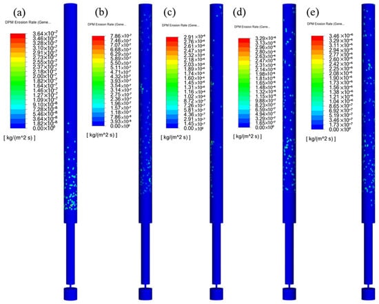
Figure 14.
Shaft erosion cloud diagram under different particle mass flow. (a) 1 × 10⁻³ kg/s; (b) 2 × 10⁻³ kg/s; (c) 3 × 10⁻³ kg/s; (d) 4 × 10⁻³ kg/s; (e) 5 × 10⁻³ kg/s.
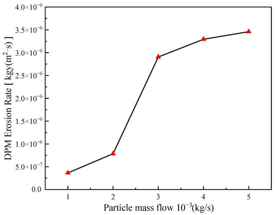
Figure 15.
Variation law of maximum erosion rate with different particle mass flow rates.
4.3. Multiple Regression Model of Erosion Rate
Polynomial fitting can not only effectively capture the interaction between independent variables, but also the form of the constructed equation facilitates direct on-site calculation. In view of this, this study adopted the polynomial regression model in response surface methodology to perform response surface layout fitting for the relationships between inlet pressure, particle diameter, particle mass flow rate, and erosion rate, and establish a corresponding prediction model. Moreover, the accuracy of the constructed polynomial was verified by means of the goodness-of-fit evaluation indicators of the regression model, as expressed by Equations (14) and (15):
where is the response value; is a constant term; is a linear coefficient; is the quadratic coefficient;
is the second-order interaction term coefficient;
is the error term; is the coefficient of determination used to evaluate the goodness of fit of the regression model; is the actual value of the dependent variable; is the predictive value of the dependent variable; and is the mean of the actual value of the dependent variable.
The three-dimensional response surface of the interaction between inlet pressure, particle diameter, and particle mass flow rate was established. The response value under any working conditions could be directly obtained by the three-dimensional response surface, and the significance of the interaction of factors on the response was analyzed. The inlet pressure and particle diameter response surface, the inlet pressure and particle mass flow response surface, and the particle diameter and particle mass flow response surface are shown in Figure 16, Figure 17 and Figure 18.
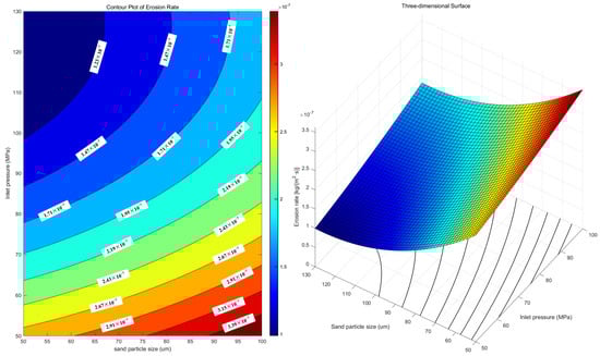
Figure 16.
Response surface of inlet pressure and particle diameter.
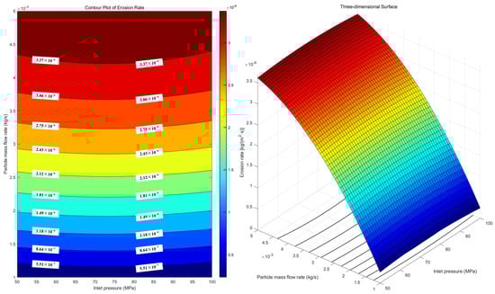
Figure 17.
Response surface of inlet pressure and particle mass flow rate.
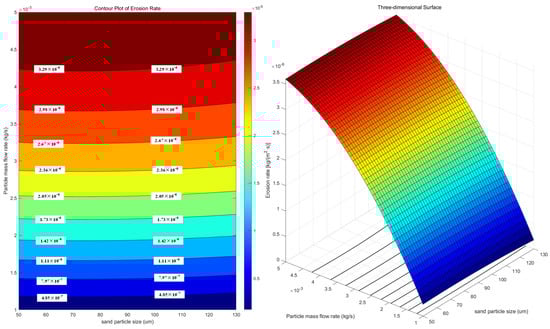
Figure 18.
Response surface of particle diameter and mass flow rate.
It can be seen from the figures that the interaction between particle mass flow and inlet pressure has the greatest influence on the erosion rate, and the interaction between inlet pressure and particle diameter has the least influence on the erosion rate. However, by comparing the response surface of inlet pressure and particle mass flow rate with the response surface of particle diameter and particle mass flow rate, it is found that the two graphs are close to each other. The particle diameter and inlet pressure have no significant effect on the erosion rate, which is consistent with the increase in the maximum erosion rate in the previous article.
Equation (16) was obtained by using the multiple regression model of the linear interaction term, and the value of R2 was 0.962941. The comparison between the actual values and the predicted values is presented in Figure 19. It can be found that the prediction of low erosion rates is better.
where is the inlet pressure, MPa; is the particle diameter, μm; and is the particle mass flow rate, g/s.
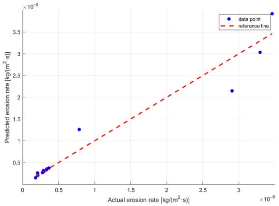
Figure 19.
Comparison of the actual values and the predicted values.
5. Conclusions
The wellbore erosion model of a high-pressure downhole throttle valve was established, and the flow field and wellbore erosion behavior of downhole throttling were simulated using Fluent. The distribution law of the pressure, temperature, and velocity fields under throttling conditions and the influences of different factors on wellbore erosion were analyzed. The multivariate regression model was used to predict the erosion trend.
- (1)
- The flow field at the nozzle changes dramatically, and there is an obvious pressure drop, temperature drop, and velocity rise. Before throttling, the pressure, temperature, and velocity in the wellbore do not change significantly. After throttling, there is an obvious pressure drop and temperature drop, and the velocity rises rapidly. The temperature drop area is basically the same as the velocity cloud area. When the surrounding gas is completely mixed, the pressure, temperature, and speed gradually stabilize.
- (2)
- The erosion shape of the wellbore outlet wall has a point-like distribution. The closer to the throttle valve outlet, the more intense the erosion point distribution is. Under the same working conditions, increasing the inlet pressure and particle mass flow rate will increase the maximum erosion rate. The increase in particle diameter will reduce the maximum erosion rate. The particle mass flow rate has the greatest influence on the maximum erosion rate. When the particle mass flow rate increases from 1 × 10⁻³ kg/s to 5 × 10⁻³ kg/s, the increase is 850.55%. The second is the particle diameter. The increase in collision frequency between particles and the wall is an important factor affecting the maximum erosion rate.
- (3)
- The multiple regression model of the linear interaction term was used to fit the erosion rate of inlet pressure, particle diameter, and particle mass flow, and the erosion trend was predicted. It was found that the particle mass flow rate has the greatest influence on the maximum erosion rate, and the fitting accuracy R2 was 0.963, which indicates a good prediction effect. It is recommended to place a sand control screen below the throttle to reduce the risk of wellbore erosion.
Author Contributions
Investigation, C.D. and R.Z.; writing—original draft, C.D.; software, C.D., X.B., and Y.H.; formal analysis, C.D.; writing—review & editing, R.K.; visualization, R.K., R.Z., and D.N.; methodology, R.K. and G.Z.; validation, R.K., X.B., D.N., G.Z., and D.Z.; data curation, X.B., Y.H., and G.Z.; supervision, R.Z.; project administration, Y.H. and D.N.; project administration, G.Z.; conceptualization, D.Z.; funding acquisition, D.Z. All authors have read and agreed to the published version of the manuscript.
Funding
This research received no external funding.
Data Availability Statement
Data are contained within the article.
Conflicts of Interest
Authors Cheng Du, Xiangwei Bai, Rong Zheng, Yao Huang, Dan Ni, Guangliang Zhou were employed by the Northwest Sichuan Division of Petro China Southwest Oil & Gas Field Company. All authors declare that there are no other competing interests.
References
- Liu, Z.; Niu, J.; Guo, Y.; Jia, Y.; Cui, M. Mechanisms of CO2 enhanced gas recovery in tight-sand gas reservoirs. Energy Geosci. 2025, 6, 100393. [Google Scholar] [CrossRef]
- Bjorlykke, K. Relationships between depositional environments, burial history and rock properties. Some principal aspects of diagenetic process in sedimentary basins. Sediment. Geol. 2014, 301, 1–14. [Google Scholar] [CrossRef]
- Tayong, A.R.; Alhubail, M.M.; Maulianda, B.; Barati, R. Simulating yield stress variation along hydraulic fracture face enhances polymer cleanup modeling in tight gas reservoirs. J. Nat. Gas Sci. Eng. 2019, 65, 32–44. [Google Scholar] [CrossRef]
- Jia, A.; Wei, Y.; Guo, Z.; Wang, G.; Meng, D.; Huang, S. Development status and prospect of tight sandstone gas in China. Nat. Dustry 2022, 9, 467–476. [Google Scholar] [CrossRef]
- Yuhual, C.; Luo, J.; Wu, C.; Hu, X.; Yang, Y.; Wei, C. A model of evaluating dynamical process of the interlayer interference of tight gas and coalbed methane and its application. Gas Sci. Eng. 2025, 134, 205528. [Google Scholar] [CrossRef]
- Iqbal, S.M.; Hu, D.; Hussain, J.; Ali, N.; Hussain, W.; Hussain, A.; Nyakilla, E.E. Integrated reservoir characterization and simulation approach to enhance production of tight sandstone gas reservoir, Sulige gas field, Ordos Basin, China. Phys. Chem. Earth Parts A/B/C 2025, 138, 103846. [Google Scholar] [CrossRef]
- Wang, Z.; Tian, L.; Huang, W.; Chen, X.; Xu, W.; Tang, C.; Chai, X.; Zhu, Y. A model for evaluating relative gas permeability considering the dynamic occurrence of water in tight reservoirs. Fuel 2025, 386, 134240. [Google Scholar] [CrossRef]
- Guo, T.; Wang, L.; Meng, X.; Shafiq, M.U.; Ci, J.; Lei, W. Layered massive fracturing of carrier beds commercially unveils the deep tight sandstone gas reserves in Sichuan Basin. Fuel 2025, 379, 133084. [Google Scholar] [CrossRef]
- Guo, J.; Lu, Q.; Liu, Z.; Zeng, F.; Guo, T.; Liu, Y.; Lin, L.; Qiu, L. Concept and key technology of “multi-scale high-density” fracturing technology: A case study of tight sandstone gas reservoirs in the western Sichuan Basin. Nat. Gas. Ind. B 2023, 10, 283–292. [Google Scholar] [CrossRef]
- Wang, L.; Li, X.; Wang, J.; Zhang, H.; Shi, H.; Liu, G.; Yang, D. Effect of pore-throat structure on irreducible water saturation and gas seepage capacity in a multilayer tight sandstone gas reservoir. Geoenergy Sci. Eng. 2025, 249, 213787. [Google Scholar] [CrossRef]
- Guo, T.; Xiong, L.; Ye, S.; Dong, X.; Wei, L.; Yang, Y. Theory and practice of unconventional gas exploration in carrier beds: Insight from the breakthrough of new type of shale gas and tight gas in Sichuan Basin, SW China. Pet. Explor. Dev. 2023, 50, 27–42. [Google Scholar] [CrossRef]
- Zhao, E.-M.; Jin, Z.-J.; Li, G.-S.; Zhang, K.-Q.; Zeng, Y. Feasibility of CO2 storage and enhanced gas recovery in depleted tight sandstone gas reservoirs within multi-stage fracturing horizontal wells. Pet. Sci. 2024, 21, 4189–4203. [Google Scholar] [CrossRef]
- Fang, B.; Ning, F.; Ou, W.; Wang, D.; Zhang, Z.; Yu, Y.; Lu, H.; Wu, J.; Vlugt, T.J.H. The dynamic behavior of gas hydrate dissociation by heating in tight sandy reservoirs: A molecular dynamics simulation study. Fuel 2019, 258, 116106. [Google Scholar] [CrossRef]
- Dai, J.; Dong, D.; Ni, Y.; Gong, D.; Huang, S.; Hong, F.; Zhang, Y.; Liu, Q.; Wu, X.; Feng, Z. Distribution patterns of tight sandstone gas and shale gas. Pet. Explor. Dev. 2024, 51, 767–779. [Google Scholar] [CrossRef]
- Rao, S.; Li, Z.; Lu, H.; Deng, Y. A review of gas hydrate formation characteristics at interfaces. Fuel 2025, 392, 134863. [Google Scholar] [CrossRef]
- Zhao, Q.; Li, X.-S.; Chen, Z.-Y.; Li, Q.-P.; He, J. Dynamic competitive co-production behaviors between natural gas hydrate and higher-pressure shallow gas under wellbore interference: An experimental study. Appl. Energy 2025, 384, 125474. [Google Scholar] [CrossRef]
- Tang, Y.; Zhang, Y.; He, Y.; Zhou, Y.; Zhao, P.; Wang, G. Study on multi-stage adjust mechanism of downhole stratification control tool for natural gas hydrate multi-gas combined production gas lift. Int. J. Hydrogen Energy 2024, 72, 800–814. [Google Scholar] [CrossRef]
- Zhang, Z.; Sun, B.; Wang, Z.; Mu, X.; Sun, D. Multiphase throttling characteristic analysis and structure optimization design of throttling valve in managed pressure drilling. Energy 2023, 262, 125619. [Google Scholar] [CrossRef]
- Abduljabbar, A.; Mohyaldinn, M.; Younis, O.; Alghurabi, A. A numerical CFD investigation of sand screen erosion in gas wells: Effect of fine content and particle size distribution. J. Nat. Gas. Sci. Eng. 2021, 95, 104228. [Google Scholar] [CrossRef]
- Deng, K.; Zhou, N.; Lin, Y.; Cheng, J.; Bing, L.; Jing, Z. Experimental and numerical study on the high-speed gas-solid nozzle erosion of choke manifold material in high pressure and high production gas well. Powder Technol. 2024, 438, 119628. [Google Scholar] [CrossRef]
- Zheng, J.; Li, J.; Dou, Y.; Hu, Z.; Yang, X.; Zhang, Y. Research on Downhole Throttling Characteristics of Gas Wells Based on Multi-Field and Multi-Phase. Processes 2023, 11, 2670. [Google Scholar] [CrossRef]
- Wang, F.; Qin, D.; Zhang, B.; He, J.; Wang, F.; Zhong, T.; Zhang, Z. Upper limit estimate to wellhead flowing pressure and applicable gas production for a downhole throttling technique in high-pressure–high-temperature gas wells. J. Pet. Explor. Prod. Technol. 2024, 14, 1443–1454. [Google Scholar] [CrossRef]
- Wang, F.; Qin, D.; Zhang, B.; Wang, F.; Zhong, T.; Shang, Z.; Cui, H. Application of downhole throttling technology to mitigate sustained casing pressure. J. Pet. Explor. Prod. Technol. 2024, 14, 1539–1551. [Google Scholar] [CrossRef]
- Huo, G.Y.; Dian, S.Y.; Xu, X. Finite Element Analysis of New Downhole Throttle Based on Orifice Valve. In Proceedings of the 3rd International Conference on Automation, Control and Robotics Engineering (Cacre 2018), Chengdu, China, 19–22 July 2018; Volume 428, p. 012016. [Google Scholar]
- Tian, J.L.; Liang, Z.; Yang, L.; Mei, X.Q.; Mei, Q.G.; Jia, Y.A. Numerical Calculation of Throttle Nozzle Diameter Influence on Downhole Choke Flow Field. Appl. Mech. Mater. 2011, 80–81, 288–293. [Google Scholar] [CrossRef]
- Xing, X.; Chen, H.; Ma, Y.; Yu, J.; Xue, D.; Zou, M.; Kou, L. Numerical study on a new adjustable multi-hole throttling device for natural gas flooding. Front. Chem. Eng. 2024, 6, 1497022. [Google Scholar] [CrossRef]
- Li, C.; Zhang, C.; Li, Z.; Jia, W. Numerical study on the condensation characteristics of natural gas in the throttle valve. J. Nat. Gas Sci. Eng. 2022, 104, 104689. [Google Scholar] [CrossRef]
- Li, Z.; Zhang, C.; Li, C.; Jia, W. Thermodynamic study on the natural gas condensation in the throttle valve for the efficiency of the natural gas transport system. Appl. Energy 2022, 322, 119506. [Google Scholar] [CrossRef]
- Ma, H.; Jiang, Y.; Yin, Q.; Zhang, F.; Chen, S.; Lv, Y.; Lei, G. Investigation on Erosion Resistance of Downhole Throttle with Ultra-high Pressure. IOP Conf. Ser. Earth Environ. Sci. 2020, 453, 012059. [Google Scholar] [CrossRef]
- Stavropoulou, M.; Papanastasiou, P.; Vardoulakis, I. Coupled wellbore erosion and stability analysis. Int. J. Numer. Anal. Methods Geomech. 1998, 22, 749–769. [Google Scholar] [CrossRef]
- Hu, X.; Li, X.; Zhou, F.; Bai, Y.; Chen, C.; Zhang, P. Simulation study on proppant transport in a horizontal wellbore considering perforation erosion. Geoenergy Sci. Eng. 2023, 231, 212282. [Google Scholar] [CrossRef]
- Shi, S.-Z.; Zhang, S.-S.; Cheng, N.; Tian, G.; Zeng, D.-Z.; Yu, H.-Y.; Wang, X.; Zhang, X. Erosion characteristics and simulation charts of sand fracturing casing perforation. Pet. Sci. 2023, 20, 3638–3653. [Google Scholar] [CrossRef]
- Zeng, D.; Wang, X.; Luo, J.; Zheng, C.; Zhang, X.; Tian, G.; Yu, H.; Li, J. Evolution features and a prediction model of casing perforation erosion during multi-staged horizontal well fracturing. Wear 2024, 556–557, 205509. [Google Scholar] [CrossRef]
- Asad, A.; Awotunde, A.A.; Jamal, M.S.; Liao, Q.; Abdulraheem, A. Simulation of wellbore erosion and sand transport in long horizontal wells producing gas at high velocities. J. Nat. Gas Sci. Eng. 2021, 89, 103890. [Google Scholar] [CrossRef]
- Fetrati, M.; Pak, A. Numerical simulation of sanding using a coupled hydro-mechanical sand erosion model. J. Rock. Mech. Geotech. Eng. 2020, 12, 811–820. [Google Scholar] [CrossRef]
- Zhang, B.; Deng, J.; Lin, H.; Xu, J.; Wang, G.; Yan, W.; Wang, K.; Li, F. Study on Erosion Model Optimization and Damage Law of Coiled Tubing. Energies 2023, 16, 2775. [Google Scholar] [CrossRef]
- Li, X.; Feng, Y.; Gray, K.E. A hydro-mechanical sand erosion model for sand production simulation. J. Pet. Sci. Eng. 2018, 166, 208–224. [Google Scholar] [CrossRef]
- Zeng, D.; Zhang, E.; Ding, Y.; Yi, Y.; Xian, Q.; Yao, G.; Zhu, H.; Shi, T. Investigation of erosion behaviors of sulfur-particle-laden gas flow in an elbow via a CFD-DEM coupling method. Powder Technol. 2018, 329, 115–128. [Google Scholar] [CrossRef]
- Shoghl, S.N.; Naderifar, A.; Farhadi, F.; Pazuki, G. Prediction of Joule-Thomson coefficient and inversion curve for natural gas and its components using CFD modeling. J. Nat. Gas Sci. Eng. 2020, 83, 103570. [Google Scholar] [CrossRef]
- Yang, Y.; He, M.; Yu, P.; Kan, C.; Wang, X.; Yu, X.; Chen, X.; Tao, S.; Zhao, C.; Duan, J.; et al. Investigation on critical erosion of gas production channel for sand carrying during injection and production process in gas storage. Geoenergy Sci. Eng. 2024, 239, 212945. [Google Scholar] [CrossRef]
Disclaimer/Publisher’s Note: The statements, opinions and data contained in all publications are solely those of the individual author(s) and contributor(s) and not of MDPI and/or the editor(s). MDPI and/or the editor(s) disclaim responsibility for any injury to people or property resulting from any ideas, methods, instructions or products referred to in the content. |
© 2025 by the authors. Licensee MDPI, Basel, Switzerland. This article is an open access article distributed under the terms and conditions of the Creative Commons Attribution (CC BY) license (https://creativecommons.org/licenses/by/4.0/).