A Low-Carbon and Economic Optimal Dispatching Strategy for Virtual Power Plants Considering the Aggregation of Diverse Flexible and Adjustable Resources with the Integration of Wind and Solar Power

Abstract

Under the dual-carbon goals, with the rapid increase in the proportion of fluctuating power sources such as wind and solar energy, the regulatory capacity of traditional thermal power generation can no longer meet the demand for intra-day fluctuations. There is an urgent need to tap into the potential of flexible load-side regulatory resources. To this end, this paper proposes a low-carbon economic optimal dispatching strategy for virtual power plants (VPPs), considering the aggregation of diverse flexible and adjustable resources with the integration of wind and solar power. Firstly, the method establishes mathematical models by analyzing the dynamic response characteristics and flexibility regulation boundaries of adjustable resources such as photovoltaic (PV) systems, wind power, energy storage, charging piles, interruptible loads, and air conditioners. Subsequently, considering the aforementioned diverse adjustable resources and aggregating them into a VPP, a low-carbon economic optimal dispatching model for the VPP is constructed with the objective of minimizing the total system operating costs and carbon costs. To address the issue of slow convergence rates in solving high-dimensional state variable optimization problems with the traditional plant growth simulation algorithm, this paper proposes an improved plant growth simulation algorithm through elite selection strategies for growth points and multi-base point parallel optimization strategies. The improved algorithm is then utilized to solve the proposed low-carbon economic optimal dispatching model for the VPP, aggregating diverse adjustable resources. Simulations conducted on an actual VPP platform demonstrate that the proposed method can effectively coordinate diverse load-side adjustable resources and achieve economically low-carbon dispatching, providing theoretical support for the optimal aggregation of diverse flexible resources in new power systems.

1. Introduction

Driven by the global energy transition and the “dual-carbon” goals, the construction of new power systems is accelerating. Traditional power systems, primarily relying on fossil fuel-based power generation, feature rigid and purely consumption-oriented load sides, resulting in a relatively simple supply-demand relationship [1]. However, with the large-scale integration of renewable energy sources and the continuous improvement of terminal energy electrification levels, profound changes have occurred in the structure and characteristics of power systems [2]. Load-side resources now exhibit a trend towards diversification, flexibility, and interactivity, making the regulation of diverse load resources a critical link in ensuring the safe and stable operation of power systems and promoting the consumption of new energy sources [3,4].

In recent years, the development of new energy sources has achieved remarkable success worldwide [5]. In China, the installed capacity of wind and solar power has surpassed that of coal-fired power, becoming a significant component of the power system. However, the intermittent and fluctuating nature of new energy sources poses significant challenges to the power grid. PV power generation is significantly affected by factors such as light intensity and weather conditions, while wind power is constrained by meteorological conditions like wind speed and direction [6,7,8]. Their power output exhibits obvious randomness and uncertainty, leading to difficulties in maintaining grid power balance and resulting in frequent occurrences of wind and solar curtailment. Meanwhile, the rapid growth of new types of loads, such as electric vehicles and distributed energy storage systems, has further exacerbated the complexity and regulation challenges of the power grid [9].

On the load side, the large-scale construction of electric vehicle (EV) charging piles has led to a rapid increase in charging loads [10]. The uncoordinated charging behavior of EVs often clusters during peak load hours, further exacerbating the peak-to-valley difference in the power grid and posing pressures on its safe and stable operation. Distributed energy storage, as a flexible resource, boasts rapid charging and discharging response capabilities, effectively mitigating the imbalance between supply and demand in the grid and among users [11]. However, its promotion and application costs are relatively high, and its business models are still in the exploratory stage. Additionally, air conditioning (AC) loads, as significant adjustable loads, account for a substantial proportion during peak summer and winter seasons. By regulating the temperature settings or start-stop times of AC units through demand response mechanisms, peak loads can be effectively reduced, and the operational efficiency of the power grid can be enhanced. Interruptible loads, through the signing of interruptible load contracts, can disconnect non-critical loads during system emergencies, providing reserve capacity for the grid. Gas turbines, as flexible power sources, can rapidly respond to fluctuations in wind and solar power outputs, yet their start-up and shut-down costs are relatively high, necessitating optimized dispatching strategies to minimize frequent start-ups and shut-downs [12,13,14].

The regulation of diverse load resources aims to achieve safe, stable, and economic operation of the power system by coordinating and optimizing various resources such as PV, energy storage, charging piles, wind power, gas turbines, interruptible loads, and AC units [15]. On the one hand, through rational regulation of these resources, it is possible to effectively mitigate fluctuations in new energy outputs, reduce the curtailment rates of wind and solar power, and enhance the consumption capacity of new energy sources. On the other hand, it can help decrease the peak-to-valley difference in the grid, reduce the demand for conventional power generation installed capacity, and improve the operational efficiency and economy of the power system. Meanwhile, the regulation of diverse load resources can also promote user-side participation in grid interactions, enabling effective interactions among generation, grid, load, and storage sectors, and driving the market-oriented reform and sustainable development of the power system. Against this backdrop, in-depth research on the regulation of diverse load resources, including PV systems, energy storage, charging piles, wind power, gas turbines, interruptible loads, and AC units, holds significant theoretical and practical implications.

As an innovative energy management model, a VPP aggregates and optimally manages diverse load resources such as PV, wind power, energy storage, charging piles, interruptible loads, and AC units distributed across various locations through information and communication technologies, forming a virtual integrated power supply system [16,17]. It not only enhances energy utilization efficiency and increases the flexibility and reliability of the power system but also participates in electricity market transactions, providing flexible regulatory capabilities for the power system and promoting the consumption of renewable energy sources. The core of a VPP lies in connecting multiple distributed energy resources through a digital platform, enabling unified dispatching and operation akin to traditional power plants. Through intelligent dispatching and optimized control, the VPP can respond in real-time to changes in grid demand, coordinating the power output and electricity consumption behaviors of various resources to achieve a balance between power supply and demand [18]. For instance, during peak output periods of PV and wind power, surplus electricity can be stored in energy storage systems or directed to charge electric vehicle charging piles. During peak load periods, electricity from the energy storage systems can be released, or electricity demand can be reduced by adjusting AC loads and interruptible loads.

Currently, countries around the world are placing significant emphasis on the development of VPPs, encouraging the aggregation of distributed PV systems, decentralized wind power, novel energy storage, adjustable loads, and other resources to provide flexible regulatory capabilities for power systems [19]. Simultaneously, they support qualified industrial enterprises and industrial parks in constructing smart microgrids to enhance the local consumption of new energy sources. With robust policy support, VPPs have seen widespread application and development. Countries such as Germany, the United States, and Australia have already accumulated rich practical experiences in the VPP domain, while China is also actively advancing the construction and demonstration applications of VPP. Therefore, conducting in-depth research on the regulation of VPPs that aggregate diverse load resources, including PV systems, energy storage, charging piles, wind power, gas turbines, interruptible loads, and AC units, holds both significant theoretical and practical implications [20]. From a theoretical perspective, it contributes to refining the regulation theories and methodologies of VPPs, thereby improving the precision and efficiency of regulation. From a practical standpoint, it can offer technical support and a decision-making basis for the actual construction and operation of VPPs, facilitating their large-scale development and commercial applications.

The plant growth simulation algorithm (PGSA), an emerging intelligent optimization algorithm, is inspired by the phototropic growth characteristics of plants. It solves optimization problems by simulating the mechanism of phototropic growth during the plant growth process [21]. In PGSA, the solution space of the optimization problem is viewed as the environment in which plants grow, with solutions corresponding to the morphological states of plant growth. The objective function values are used to measure the “dominance” or “fitness” of plant growth. By simulating the process of plants bending towards light due to uneven auxin distribution, the algorithm guides the search direction towards regions with better objective function values, thereby gradually approaching the global optimal solution. The main advantages of PGSA lie in its search mechanism, which is based on the natural laws of plant growth, granting it strong adaptability and robustness [22,23]. It can effectively conduct global searches in complex solution spaces, avoiding being trapped in local optimal solutions. Additionally, the algorithm structure of PGSA is relatively simple, making it easy to understand and implement. It does not require complex mathematical derivations or parameter settings, thus lowering the application threshold of the algorithm. Therefore, PGSA demonstrates applicability in both continuous and discrete optimization problems, offering broad application prospects [24,25,26].

However, as the requirements for solution accuracy and efficiency in optimization problems continue to rise, traditional PGSA has gradually exposed certain shortcomings. For instance, when dealing with high-dimensional and complex optimization problems, the search speed of PGSA may slow down, and its convergence performance may decline [27]. Additionally, the algorithm is prone to becoming trapped in local optimal solutions during the later stages of the search, leading to less-than-ideal solution results. For certain specific types of optimization problems, there is a lack of clear guidance principles for parameter selection in PGSA, which affects the algorithm’s performance and stability. Consequently, these issues have restricted the further promotion and development of PGSA in practical applications [28,29,30].

To overcome the limitations of the traditional PGSA and fully leverage its advantages, this paper proposes an improved version of the algorithm and applies it to the low-carbon economic optimal dispatching of VPPs that aggregate diverse flexible and adjustable resources. The main contributions of this paper are as follows:

(1)

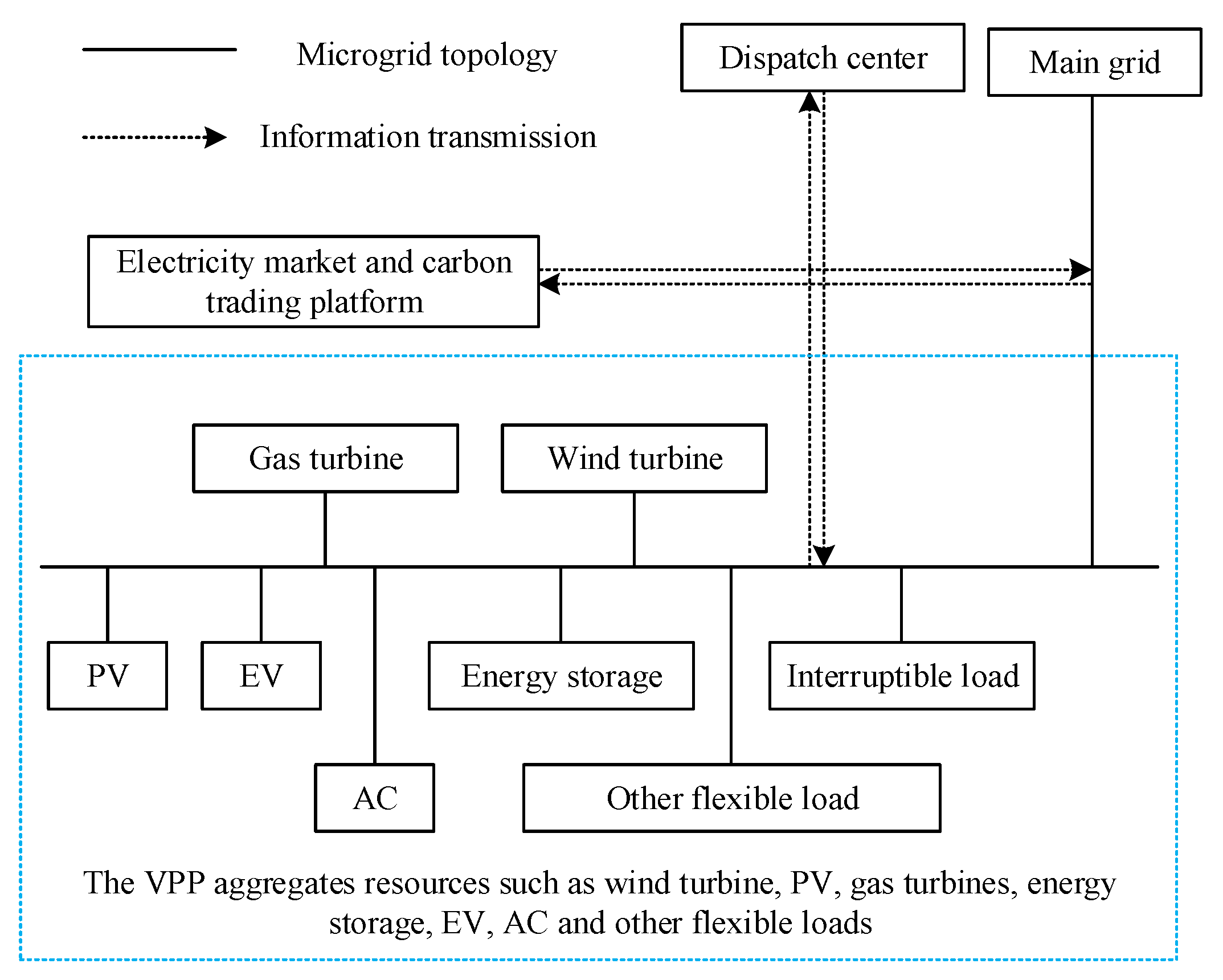
By analyzing the dynamic response characteristics and flexibility regulation boundaries of multiple adjustable resources, including PV systems, wind power, energy storage, charging piles, interruptible loads, and AC units, mathematical models for each of these resources are established.

(2)

Considering the aforementioned diverse flexible and adjustable resources and aggregating them into the VPP, a low-carbon economic optimal dispatching model for the VPP is constructed with the objective of minimizing the total system operating cost and carbon cost.

(3)

To address the slow convergence rate of the traditional PGSA when solving optimization problems with high-dimensional state variables, this paper proposes an improved PGSA by incorporating an elite selection strategy for growth points and a multi-base point parallel optimization strategy.

(4)

The improved PGSA is utilized to solve the low-carbon economic optimal dispatching model for the VPP that aggregates diverse flexible and adjustable resources, and the proposed method is validated through simulation experiments.

2. Mathematical Models of Multiple Flexible and Adjustable Resources

In this paper, the specific scope and selection criteria of “multi-type flexible and adjustable resources” for VPP are mainly aimed at PV, wind turbine, energy storage, electric vehicle, gas turbines, interruptible loads, and air conditioners in the distribution network, all of which are flexible and adjustable resources in the distribution network [13,14].

2.1. The Mathematical Model of PV

The power generation output of distributed PV is influenced by factors such as solar irradiance, real-time ambient temperature, and the soiling condition of PV panels, and its output model is represented by the following formula:

$$P_{pv}(t)=P_{pv,rated}{\delta }_{pv}\left[1+{\theta }_{pv}(T_{pv}(t)-T_{pv,rated})\right]{\displaystyle \frac{L_{pv}(t)}{L_{pv,rated}}}$$

(1)

where $P_{pv}(t)$ represents the power of distributed photovoltaic system at time t; $P_{pv,rated}$ represents the rated power of distributed photovoltaic system under standard test conditions; ${\delta }_{pv}$ represents the fouling status of distributed photovoltaic panels, and generally takes the value of 0.9; $L_{pv}(t)$ represents the light intensity at time t; $L_{pv,rated}$ is the illumination intensity under standard test conditions; ${\theta }_{pv}$ is the power compensation coefficient; $T_{pv}(t)$ represents the temperature of the distributed photovoltaic panel at time t; $T_{pv,rated}$ represents the reference temperature under standard measurement conditions, which is generally taken as 25 °C.

2.2. The Mathematical Model of Wind Turbine

For wind turbines, the probability density function of wind speed is usually expressed by establishing a two-parameter Weibull distribution, as shown in the following formula:

$$f_w(v_w)=\left({\displaystyle \frac{k_w}{v_w}}\right)\times {\left({\displaystyle \frac{v_w}{c_w}}\right)}^{k_w-1}\exp \left[-{\left({\displaystyle \frac{v_w}{c_w}}\right)}^{k_w}\right]$$

(2)

where v_w is the wind speed; c_w represents the scale parameter of Weibull distribution function, which can be used to describe the average wind speed in the area where decentralized wind power is located; k_w represents the shape parameter of Weibull distribution; and f_w(v_w) is the probability density function of wind speed.

Given a fixed wind speed, a quantitative relationship between the power generation of a wind turbine and the local wind speed can be established by fitting a model using a large amount of actual data. The following formula represents the relationship model between the power output of a wind turbine generator system and the actual local wind speed:

$$\left\{\begin{array}{c}\hfill P_w=C_w({\lambda }_w,{\beta }_w)\times {\displaystyle \frac{\rho \pi R^2}{2}}\times v_w^2\hfill \\ \hfill C_w({\lambda }_w,{\beta }_w)=0.22\times ({\displaystyle \frac{116}{{\lambda }_1}}-0.4{\beta }_w-5)\exp ({\displaystyle \frac{12.5}{{\lambda }_1}})\hfill \\ \hfill {\lambda }_1=1/({\displaystyle \frac{1}{{\lambda }_w+0.08{\beta }_w}}-{\displaystyle \frac{0.035}{1+{\beta }_w^3}})\hfill \end{array}\right.$$

(3)

where $P_w$ represents the power generation of wind turbines; $C_w({\lambda }_w,{\beta }_w)$ represents the conversion coefficient of wind turbines; ${\lambda }_w$ and ${\beta }_w$ represent the conversion parameters of fan power, respectively; $\rho$ is the air density; R represents the ratio of the blade tip speed of the wind turbine to the wind speed; and ${\lambda }_1$ is the process parameters.

2.3. The Mathematical Model of Energy Storage

The energy storage system consists of an energy storage battery bank, an energy storage energy management system, and an energy storage power control system. There exist the following mathematical relationships between its capacity and charge/discharge power:

$$E_{es}(t)=(1-{\delta }_{es})E_{es}(t-1)+\left[P_{es,ch}(t){\eta }_{es,ch}-{\displaystyle \frac{P_{es,dis}(t)}{{\eta }_{es,dis}}}\right]\Delta t$$

(4)

where $E_{es}(t)$ and $E_{es}(t-1)$ represent the amount of electricity stored in the electric energy storage at time t and time t − 1; ${\delta }_{es}$ represents the system self-discharge ratio of energy storage; $P_{es,ch}(t)$ represents the power of the energy storage in the charging state; $P_{es,dis}(t)$ represents the power of the energy storage in the discharge state; ${\eta }_{es,ch}$ represents the charging efficiency of energy storage; ${\eta }_{es,dis}$ represents the discharging efficiency of energy storage; and $\Delta t$ represents the time interval.

By establishing the mathematical relationship between the SOC of the energy storage battery and the charge/discharge power of the energy storage system, a mathematical model for the electrical energy storage system can be developed. The following equation represents the mathematical model for the SOC of the energy storage battery and the charge/discharge power of the energy storage:

$$\left\{\begin{array}{l}SOC(t)=(1-{\delta }_{es})SOC(t-1)+P_{es,ch}(t){\eta }_{es,ch}\Delta t/E_{es}(t)\\ SOC(t)=(1-{\delta }_{es})SOC(t-1)+P_{es,dis}(t)\Delta t/\left[E_{es}(t){\eta }_{es,dis}\right]\end{array}\right.$$

(5)

where SOC (t) represents the state of charge (SOC) of the energy storage at time t; SOC (t − 1) represents the SOC of the energy storage at time (t − 1).

2.4. Charging and Discharging Model of Electric Vehicle

The charging power of the EV should be less than or equal to the rated power of the charging station (CS), and the charging power can be controlled, as is shown in the following formula:

$$\left\{\begin{array}{l}{c}_{rate,E_{no}}<P_{rated}\\ c_{rate,E_{no}}^{\min }<c_{rate,E_{no}}<c_{rate,E_{no}}^{\max }\end{array}\right.$$

(6)

where $P_{rated}$ is the rated power of CS; $c_{rate,E_{no}}^{\max }$ and $c_{rate,E_{no}}^{\min }$ are the maximum and minimum charging power of the EV; $c_{rate,E_{no}}$ is the charging power of the EV.

The SOC of the EV battery should be within the specified range of 20~90%:

$$20\%\le S_{E_{no}}^s\le 90\%$$

(7)

where $S_{E_{no}}^s$ is the SOC of EV battery.

The charging and discharging strategies of the EV can be summarized as follows:

$$\left\{\begin{array}{l}{T}_{E_{no}}=[T_{E_{no}}^1,...,T_{E_{no}}^{s_{in}},...,T_{E_{no}}^{s_{out}},...,T_{E_{no}}^s]\\ T_{E_{no}}^s=\left\{\begin{array}{l}1, \mathrm{charging}\\ -1, \mathrm{discharging}\\ 0, \mathrm{else}\end{array}\right.\end{array}\right.$$

(8)

where $s_{in}$ is the time period when the EV enters the CS; $s_{out}$ is the time period when the EV leaves the CS; $T_{E_{no}}^s$ is the charging and discharging strategy; $T_{E_{no}}$ is the strategy matrix.

2.5. The Mathematical Model of Gas Turbine

A gas turbine is a widely utilized power generation device, and it operates by combusting gas to produce high-temperature and high-pressure gas, which drives a turbine wheel to rotate, thereby generating mechanical energy. This mechanical energy is then converted into electrical energy. The following outlines the operational model of a gas turbine:

$$P_{gas}(t)={\eta }_{gas}{L}_{gas}{V}_{gas}(t)$$

(9)

where $P_{gas}(t)$ denotes the output power of the gas turbine at time t; ${\eta }_{gas}$ represents the power generation efficiency of the gas turbine; $L_{gas}$ stands for the lower heating value of natural gas; and $V_{gas}\left(t\right)$ indicates the volume of natural gas consumed by the gas turbine at time t.

2.6. The Mathematical Model of Interruptible Load

For interruptible load, its model can be expressed as follows:

$$\left\{\begin{array}{l}{P}_{r,i}^{t+1}=(1-z_{r,i}^t)P_{r,i}^t\\ z_{r,i}^t\le z_r^{\max }\\ {\displaystyle \sum _{t\notin T_{r,i}}{z}_{r,i}^t}=0\\ T_{r,i}=\left[t_{r,i}^{start},t_{r,i}^{end}\right]\end{array}\right.$$

(10)

where $P_{r,i}^{t+1}$ and $P_{r,i}^t$ are the power of interruptible load of bus i at time t + 1 and t, respectively; $z_{r,i}^t$ is the interruption ratio of interruptible load of bus i at time t; $z_r^{\max }$ is the maximum value of interruptible ratio; $T_{r,i}$ is the interruption period of interruptible load of bus i; and $t_{r,i}^{start}$ and $t_{r,i}^{end}$ are the beginning and the end of $T_{r,i}$ respectively.

2.7. The Mathematical Model of AC

As a type of interruptible load, air conditioning load plays an important role in the regulation of virtual power plants, so this paper models the air conditioning load separately. A variable-frequency air conditioner adjusts the cold/hot air intake by changing the speed of the compressor, so as to continuously adjust the load and dynamically adapt to the change of room temperature; its load characteristics can be expressed as follows:

$$\left\{\begin{array}{l}{G}_1/G_2=n_1/n_2\\ H_1/H_2={\left(n_1/n_2\right)}^2\\ P_1/P_2={\left(n_1/n_2\right)}^3\end{array}\right.$$

(11)

where n₁ is the electrode speed of the chilled water pump; n₂ is the electrode speed of the cooling water pump; G₁ is the chilled water flow rate; G₂ is the cooling water flow rate; H₁ is the chilled water pump head; H₂ is the cooling water pump head; P₁ is the chilled water pump shaft power; P₂ is the cooling water pump shaft power.

The speed formula of the motor is as follows:

$$n_{ac}=60f(1-s_{ac})/p_{ac}$$

(12)

where n_ac represents the motor speed; f represents the power frequency; p_ac is the polar logarithm; and s_ac is the slip rate.

The frequency range of a conventional variable-frequency air conditioner is 10~150 Hz, and the system shall meet the following conditions:

$$\left\{\begin{array}{l}{H}_{\min }\le H\le H_{\max }\\ G_{\min }\le G\le G_{\max }\end{array}\right.$$

(13)

where H represents the pump head; H_max and H_min represent the maximum and minimum pump head, respectively; G represents water flow; G_max and G_min represent the maximum and minimum water flow, respectively.

The indoor temperature and outdoor temperature have the following relationship when the air conditioner is turned on:

$$T_{in}^{t+1}=T_{out}^{t+1}-{\eta }_{ac}{P}_{ac}{R}_{ac}-(T_{out}^{t+1}-{\eta }_{ac}{P}_{ac}{R}_{ac}-T_{in}^t)\exp (-{\displaystyle \frac{\Delta t}{R_{ac}{C}_{ac}}})$$

(14)

where $T_{in}^{t+1}$ represents the indoor temperature at time t + 1; $T_{out}^{t+1}$ represents the outdoor temperature at time t + 1; ${\eta }_{ac}$ is the energy efficiency ratio of air conditioning; P_ac is the air conditioning power; R_ac is the equivalent thermal resistance; $T_{in}^t$ represents the indoor temperature at time t; C_ac is the equivalent heat capacity; and $\Delta t$ is the time interval.

3. Optimal Dispatching Model for the VPP Aggregating Diverse and Flexibly Adjustable Resources

The core mechanism of low-carbon economic optimal scheduling model for VPPs is to aggregate dispersed and distributed energy resources into a whole that can be managed in a unified and coordinated way through advanced information and communication technology. Under the premise of meeting the constraints of power system operation, the optimal coordinated scheduling of these resources is achieved with the goal of the lowest total operating cost and the lowest total carbon emission. In this paper, after all kinds of flexible and adjustable resources are aggregated, the operation cost and carbon emission cost are considered at the same time, and the optimization model is established with the goal of minimizing the total operation cost and carbon emission cost of the system.

3.1. The Objective Function

The objective in this paper is to minimize the total system operating cost and carbon cost, which is shown as follows:

$$\min \hspace{0.17em}{C}_{total}=C_{operation}+C_{carbon}$$

(15)

$$C_{operation}={\displaystyle \sum _{t=1}^{24}\left[C_{grid}(t)+C_{gas}(t)+C_{es}(t)+C_r(t)+C_{penalty}(t)\right]}$$

(16)

where $C_{total}$ is the total system operating cost and carbon cost; $C_{operation}$ is the operating cost; C_carbon is the carbon cost; C_grid(t) represents the interaction cost of the power grid at time t; C_gas(t) represents the power generation cost of the gas turbine at time t; C_es(t) represents the cost of the energy storage system at time t; C_r(t) represents the interruptible load compensation cost at time t; C_penalty(t) represents the penalty cost of abandoning wind and light.

The detailed calculation expressions of the above costs are as follows:

$$\left\{\begin{array}{l}{C}_{grid}(t)={\lambda }_{buy}(t)P_{buy}(t)-{\lambda }_{sell}(t)P_{sell}(t)\\ C_{gas}(t)=a_{gas}{P}_{gas}(t)+b_{gas}\\ C_{es}(t)={\rho }_{ch}{P}_{ch}(t)+{\rho }_{dis}{P}_{dis}(t)\\ C_r(t)={\eta }_r{P}_r(t)\\ C_{penalty}(t)={\gamma }_{pv}\left[P_{pv,pre}(t)-P_{pv}(t)\right]+{\gamma }_w\left[P_{w,pre}(t)-P_w(t)\right]\\ C_{carbon}={\gamma }_{c{o}_2}(E_{c{o}_2}-E_{allow})\\ E_{c{o}_2}={\displaystyle \sum _{t=1}^{24}{\phi }_{gas}{P}_{gas}(t)+{\phi }_{grid}{P}_{buy}(t)}\end{array}\right.$$

(17)

where ${\lambda }_{buy}(t)$ and ${\lambda }_{sell}(t)$ represent the purchase/sale price at time t, respectively; $P_{buy}(t)$ and $P_{sell}(t)$ represent the purchase/sale power at time t, respectively; $P_{gas}(t)$ stands for gas turbine power at time t; $a_{gas}$ and $b_{gas}$ stand for the fuel cost coefficient, respectively; $P_{ch}(t)$ and $P_{dis}(t)$ represent the charging and discharging power of energy storage at time t, respectively; ${\rho }_{ch}$ and ${\rho }_{dis}$ represent the loss cost coefficient of charging and discharging, respectively; $P_r(t)$ represents the interruptible load power at time t; ${\eta }_r$ represents the compensation price of interruptible load; ${\gamma }_{pv}$ and ${\gamma }_w$ represent the penalty cost coefficient of abandoning wind and light, respectively; $P_{pv}(t)$ and $P_w(t)$ represent the actual power of wind and light, respectively; $P_{pv,pre}(t)$ and $P_{w,pre}(t)$ represent the predicted power of photovoltaic and wind, respectively; ${\gamma }_{c{o}_2}$ represents the carbon price; $E_{c{o}_2}$ represents the carbon emissions; $E_{allow}$ stands for the carbon emission quota; ${\phi }_{gas}$ represents the power carbon emission factor of the gas turbine; and ${\phi }_{grid}$ represents the carbon emission factor of the power grid.

3.2. The Constraints

The constraint conditions of various flexible and adjustable resources in the system are as follows:

$$0\le P_{pv}(t)\le P_{pv,pre}(t)$$

(18)

$$0\le P_w(t)\le P_{w,pre}(t)$$

(19)

$$P_{gas,\min }\le P_{gas}(t)\le P_{gas,\max }$$

(20)

$$\left|P_{gas}(t)-P_{gas}(t-1)\right|\le R_{gas}$$

(21)

$$\left\{\begin{array}{l}0\le P_{ch}(t)\le P_{es,ch}^{\max }\\ 0\le P_{dis}(t)\le P_{es,dis}^{\max }\\ E_{es}^{\min }\le E_{es}(t)\le E_{es}^{\max }\\ P_{ch}(t)\times P_{dis}(t)=0\end{array}\right.$$

(22)

$${\displaystyle \sum _{t=1}^{24}{P}_{ev}(t)}=E_{ev}^{total}$$

(23)

$$0\le P_r(t)\le P_r^{\max }(t)$$

(24)

$$\left\{\begin{array}{l}{T}_{in}^{\min }\le T_{in}(t)\le T_{in}^{\max }\\ P_{ac}^{\min }\le P_{ac}(t)\le P_{ac}^{\max }\end{array}\right.$$

(25)

$$\left\{\begin{array}{l}{P}_{buy}(t)\ge 0\\ P_{sell}(t)\ge 0\\ P_{buy}(t)\times P_{sell}(t)=0\end{array}\right.$$

(26)

$$\begin{array}{l}{P}_{pv}(t)+P_w(t)+P_{gas}(t)+P_{dis}(t)+P_{buy}(t)=\\ P_{load}(t)+P_{ev}(t)+P_{ac}(t)+P_{ch}(t)-P_r(t)+P_{sell}(t)\end{array}$$

(27)

where $P_{gas}(t-1)$ stands for gas turbine power at time t − 1; R_gas represents the climbing rate of the gas turbine; $P_{es,ch}^{\max }$ and $P_{es,dis}^{\max }$ represent the maximum charging and discharging power, respectively; $E_{es}^{\max }$ and $E_{es}^{\min }$ represent the maximum and minimum energy storage capacity, respectively; $P_{ev}(t)$ is the charging power of the EV at time t; $E_{ev}^{total}$ is the battery capacity of EV; $P_r(t)$ is the power of the interruptible load at time t; $P_r^{\max }(t)$ is the maximum power of the interruptible load at time t; $T_{in}(t)$ represents the indoor temperature at time t; $P_{ac}(t)$ is the power of the AC at time t; $T_{in}^{\max }$ and $T_{in}^{\min }$ represents the maximum and minimum indoor temperature at time t; $P_{ac}^{\max }$ and $P_{ac}^{\min }$ represents the maximum and minimum power of the AC at time t; $P_{load}(t)$ represents the power of the load at time t.

4. The Improved Plant Growth Simulation Algorithm for the Dispatching of VPPs

4.1. The Plant Growth Simulation Algorithm

The PGSA simulates the phototropism of plant growth by establishing a probabilistic model. This model utilizes morphogen concentration to determine which growth point is granted priority for growth. Morphogens are growth hormones within cells, and their concentration dictates whether a cell can produce new branches during division, with values ranging between 0~1. After a new branch emerges, the morphogen concentrations of all growth points need to be recalculated in the new environmental context. In the probabilistic model, a function f(y) is employed to describe the growth environment of a growth point y. A smaller function value of f(y) indicates a better growth environment for the growth point y, making it more likely to generate new branches. The model can be described as follows: Starting from a root node x₀, a trunk M grows. Suppose there are k growth points S_M1, S_M2, ..., S_Mk on M that are superior to the root node x₀ in terms of growth environment, i.e., f(x₀) > f(S_Mi), for i = 1, 2, 3, ..., k. The morphogen concentrations P_M1, P_M2, ..., P_Mk of the growth points S_M1, S_M2, ..., S_Mk can be calculated using the following formula:

$$\left\{\begin{array}{l}{P}_{Mi}={\displaystyle \frac{f(x_0)-f(S_{Mi})}{{\displaystyle \sum _{i=1}^{k}f(x_0)-f(S_{Mi})}}}\\ {\displaystyle \sum _{i=1}^k{P}_{Mi}}=0\end{array}\right.$$

(28)

Then, a random number r₀ is selected from the interval (0, 1). This random number, akin to a ball landing in one of the state spaces corresponding to P_M1, P_M2, ..., P_Mk, determines which growth point within that space will be granted priority for growth in the next iteration. This point is referred to as the base point. For instance, if S_Mu is the point that obtains the priority for growth, then r₀ must satisfy the following condition:

$${\displaystyle \sum _{i=1}^{u-1}{P}_{Mi}}<r_0\le {\displaystyle \sum _{i=1}^u{P}_{Mi}}$$

(29)

Suppose the random number r₀ falls into the state space corresponding to P_M2, i.e.,:

$${\displaystyle \sum _{i=1}^1{P}_{Mi}}<r_0\le {\displaystyle \sum _{i=1}^2{P}_{Mi}}$$

(30)

The growth point S_M2 generates a new branch m. Suppose there are q growth points S_m1, S_m2, ..., S_mq on branch m that are superior to the root node x₀, with corresponding morphogen concentrations P_m1, P_m2, ..., P_mq. At this point, not only do the growth points on branch m need to have their morphogen concentrations calculated, but the growth points on trunk M excluding S_M2 also need to have their morphogen concentrations recalculated. The morphogen concentrations of these k + q growth points can be calculated using the following formula:

$$\left\{\begin{array}{l}{P}_{Mi}={\displaystyle \frac{f(x_0)-f(S_{Mi})}{{\displaystyle \sum _{i=1,i\ne 2}^{k}f(x_0)-f(S_{Mi})}+{\displaystyle \sum _{j=1}^{q}f(x_0)-f(S_{mj})}}},\hspace{1em}i=1,2,\dots ,k\\ P_{mj}={\displaystyle \frac{f(x_0)-f(S_{mj})}{{\displaystyle \sum _{i=1,i\ne 2}^{k}f(x_0)-f(S_{Mi})}+{\displaystyle \sum _{j=1}^{q}f(x_0)-f(S_{mj})}}},\hspace{1em}j=1,2,\dots ,q\\ {\displaystyle \sum _{i=1,i\ne 2}^k{P}_{Mi}}+{\displaystyle \sum _{j=1}^q{P}_{mj}}=0\end{array}\right.$$

(31)

At this point, all the growth points on the trunk M and the branch m form a new state space of morphogen concentrations. The acquisition of the next new base point follows the same process as that for S_M2. This process is repeated until no new branches are generated. The growth points represent feasible solutions to the problem, f(y) represents the objective function, the lengths of the trunk and branches denote the search regions for feasible solutions, and the root of the tree represents the initial solution. By applying the phototropic growth process of plants in this manner, we can adapt it to solve optimization problems.

4.2. The Improved Plant Growth Simulation Algorithm

In the traditional PGSA, the growth points on the trunk and branches are only compared with the initial solution (the tree root). As the number of iterations increases, numerous growth points emerge within the plant growth system. The probability of selecting faster-evolving growth points (hereinafter referred to as elite growth points) diminishes, thereby affecting the algorithm’s convergence speed. Moreover, the next base point is determined through random numbers. Before an elite growth point is chosen as the base point, some inferior growth points may be selected, consuming unnecessary runtime and potentially preventing the algorithm from finding the optimal solution within a limited number of iterations. Additionally, the algorithm selects only one base point for iterative search at a time, which reduces its operational efficiency to some extent. The termination condition of the traditional algorithm is that when the plant grows to its complete state and no new branches sprout, and the algorithm is deemed to have ended. However, generally speaking, there is no need to wait for the plant to grow completely to find the optimal solution, which also results in wasted computational time.

In response to the aforementioned issues, this paper proposes an improved PGSA. The specific improvements are as follows:

(1)

To accelerate the algorithm’s computational speed, an elite selection strategy is introduced. Each newly generated growth point is compared with the optimal solution among the current feasible solutions. If it is superior to the current optimal solution, it is retained in the growth point list; otherwise, it is discarded. That is,

$$f(x_0^{\ast })>f(S_{Mi}),\hspace{1em}i=1,2,\dots ,k$$

(32)

where $f(x_0^{\ast })$ is the current local optimal value; $x_0^{\ast }$ is the base point corresponding to the current local optimal value.

(2)

The optimal solution for an optimization problem is often obtained by the evolution of a better local solution. Therefore, select a number of better elite growth points as the base points rather than using random selection, which can not only improve the solution speed of the algorithm but also improve the stability of the algorithm.

(3)

Select multiple elite growth points as the base points at a time, so that they can evolve at the same time, thus speeding up the search rate.

(4)

Set termination conditions as follows: ① When the number of operations reaches the maximum number of iterations, the algorithm terminates the iteration. ② When the growth point list is empty, it is considered that the plant has fully grown, and the algorithm terminates the iteration. ③ Set the initial solution as X_best. When the current optimal solution is better than X_best, set X_best equal to the current optimal solution. If the current optimal solution remains unchanged within a certain number of runs, the algorithm terminates the iteration.

The calculation flow chart of the improved PGSA is shown in Figure 1.

The computational process of the modified PGSA is as follows:

(1)

Input the basic data.

(2)

Define the search area and determine the solution space; set the iteration count T = 0.

(3)

Select the initial solution x_T as the tree root and calculate the initial value of the objective function.

(4)

Set x_best equal to the initial value x_T as the optimal feasible solution, and F_best as the function value of x_best, i.e., x_best = x_T, F_best = f(x_T).

(5)

Centered around x_T, simulate the plant growth to generate new feasible solutions x_p, and calculate their corresponding objective function values f(x_p). If f(x_p) > f(x_T), discard the point; otherwise, retain it in the set of feasible solutions.

(6)

Among the obtained feasible solutions, identify the local optimal solution x_pbest. If f(x_pbest) < F_best, set x_best = x_pbest and F_best = f(x_pbest).

(7)

Arrange all feasible solutions in the growth point list in ascending order based on their objective function values, and select the top s feasible solutions as the base points for the next iteration.

(8)

When the iteration count T is greater than or equal to the maximum iteration count T_max or when the current optimal solution is no longer updated, terminate the algorithm and output the final results. Otherwise, set T = T + 1 and return to step (5).

5. Numerical Test and Analysis

5.1. Basic Data and Simulation Conditions

This paper conducts a simulation by using an actual VPP in China to validate the effectiveness of the proposed method. The VPP used in this paper is the actual VPP of a new power load management system that has been built in China and has been actually connected to China State Grid. The schematic diagram of this VPP model is illustrated in Figure 2. This VPP aggregates resources such as wind turbine generators, PV, gas turbines, energy storage devices, and flexible loads. The VPP control center is capable of exchanging information with institutions like carbon trading platforms and electricity markets, enabling effective energy interaction and more efficient and reliable energy management. When there is an excess or shortage of energy supply in the VPP, it can engage in transactions with various energy trading centers to meet users’ energy demands. The simulation environment is based on MATLAB R2014a. The branching probability for the PGSA is set to 0.2, the maximum number of iterations is set to 150, and the number of initial growth base points is set to 5.

Table 1. The time-of-use electricity purchase and sale prices in the power market.

Period of Time	Period	Purchase Price (RMB/MWh)	Sale Price (RMB/MWh)
Peak period	08:00–11:00; 16:00–21:00	962.6	528.5
Normal period	06:00–08:00; 11:00–16:00; 21:00–23:00	697.5	352.4
Valley period	00:00–06:00; 23:00–24:00	327.8	176.2

presents the time-of-use electricity purchase and sale prices in the power market when this VPP interacts with the grid.

5.2. Simulation Results and Analysis

To validate the effectiveness of the proposed method in this paper, a comparison was conducted between the proposed method and the particle swarm optimization (PSO) algorithm, genetic algorithm (GA), and the traditional PGSA. The simulation results are presented in

Table 2. Comparison of optimization results of different algorithms.

Algorithm	Total Cost (RMB)	Iterations	Time (s)
PSO	6458.77	135	20.17
GA	6235.48	118	17.54
PGSA	6366.42	126	18.63
The proposed method	6072.83	107	16.21

. As shown in Table 2, after optimization by the PSO algorithm, the total operating cost of the system is 6458.77 RMB, with 135 iterations and a total simulation runtime of 20.17 s. Following optimization by the GA algorithm, the total operating cost is 6235.48 RMB, with 118 iterations and a runtime of 17.54 s. For the traditional PGSA algorithm, the optimized total operating cost is RMB 6366.42, with 126 iterations and a runtime of 18.63 s. In contrast, after optimization by the proposed method in this paper, the total operating cost is RMB 6072.83, with 107 iterations and a runtime of 16.21 s. It can thus be observed that, compared with the PSO, GA, and traditional PGSA algorithms, the proposed method, after strategy optimization based on the traditional PGSA, achieves reductions in both the number of iterations and runtime. Moreover, it yields the best optimization results among the four algorithms. This demonstrates that the proposed method can effectively solve the VPP optimization model with the integration of diverse wind and solar resources presented in this paper.

After optimizing and solving the optimization model of VPP by using the method proposed in this paper, the output power of each energy source within the system is illustrated in Figure 3. Figure 3 provides a detailed depiction of the energy dispatch output for the VPP over a 24 h period. As shown in Figure 3, the wind power remains relatively stable. The solar power reaches its peak at noon (12:00) and 1:00 PM, with lower outputs in the morning and evening, and zero output after sunset. The gas turbine operates from 6:00 AM to 9:00 PM, maintaining a relatively constant power output. The interaction between the VPP and the main grid primarily involves purchasing power from the grid during the night when electricity prices are low, and selling excess power back to the main grid during the day, particularly during periods of high solar power generation. The energy storage system charges during off-peak hours when electricity is cheaper and discharges during peak hours to capitalize on the price difference between peak and off-peak periods, thereby generating profits.

In order to analyze the impact of carbon trading and energy storage on the economic operation of VPP, this paper incorporates carbon trading costs into the total cost and the following three scenarios are set up and compared:

Scenario 1: neither carbon trading nor energy storage are involved in the economic operation of the VPP.

Scenario 2: only carbon trading is involved in the economic operation of the VPP.

Scenario 3: both carbon trading and energy storage are involved in the economic operation of the VPP.

To study and analyze the economic and environmental indicators under the three scenarios, the VPP economic operation models for each scenario are optimized and calculated, and the results are presented in

Table 3. The economic and environmental indicators under the three scenarios.

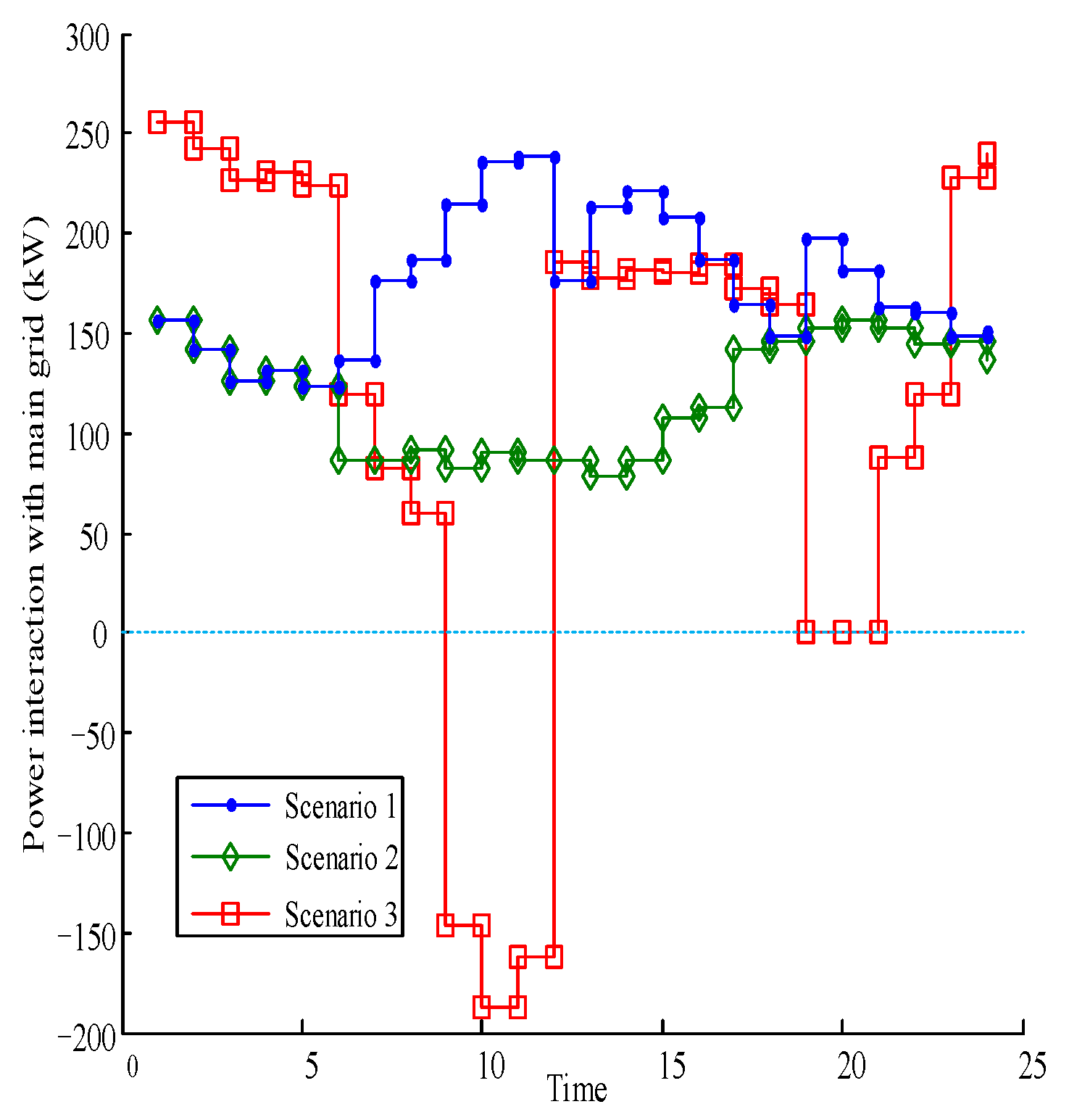
Scenario	Total Cost (RMB)	Carbon Trading Cost (RMB)	Operation Cost (RMB)	Carbon Emissions (t)
Scenario 1	6213.57	0	6213.57	1.5142
Scenario 2	6287.64	385.32	5902.32	1.3379
Scenario 3	6072.83	367.41	5705.42	1.2757

.

As shown in Table 3, in scenario 1, the total system cost is RMB 6213.57. Since carbon trading is not involved in scenario 1, the carbon trading cost is 0, and the total cost is entirely the system’s operating cost, and the carbon emissions in this scenario amount to 1.5142 tons. In scenario 2, the total system cost is RMB 6287.64, which includes a carbon trading cost of RMB 385.42 and an operation cost of RMB 5902.32. Additionally, the carbon emissions in this scenario are 1.3379 tons. Due to the consideration of carbon trading costs, the total system cost in scenario 2 increases compared to scenario 1, but the carbon emissions are lower. In scenario 3, the total system cost is RMB 6072.83, comprising a carbon trading cost of RMB 367.41 and an operation cost of RMB 5705.42. Moreover, the carbon emissions in this scenario are 1.2757 tons. Thanks to the proposed method in this paper, namely scenario 3, which takes into account both the carbon trading mechanism and the participation of energy storage, it can maximize benefits, reduce system costs, and lower carbon emissions during the optimization of diverse energy resources.

In this paper, the carbon trading mechanism sets a price for carbon emissions, internalizing environmental costs into economic costs. This raises the costs of high-carbon power sources while enhancing the economic viability of low-carbon power sources, providing direct economic incentives for carbon reduction. By assigning a clear price to carbon emissions, carbon trading introduces carbon costs that significantly boost the competitiveness and relative economic efficiency of renewable energy sources such as wind and solar power, as well as energy storage systems. This gives VPPs a direct economic impetus to reduce the use of high-carbon power sources and increase the consumption and utilization of clean energy when optimizing dispatch to minimize total operational costs. Energy storage systems offer critical capabilities for energy time-shifting and rapid power regulation, enabling VPPs to proactively leverage fluctuations in electricity prices and carbon intensity/carbon prices over time. Therefore, when considering both carbon costs and the flexibility provided by energy storage, the decision making logic for VPP optimization and dispatch undergoes a fundamental transformation. Acting as the “brain” of operations, under carbon cost constraints, VPPs fully utilize the flexibility of energy storage to dynamically select the combination of generation, power purchase, and charging/discharging at each moment that results in the lowest total cost. The core decision making logic shifts to prioritizing the utilization of low-carbon resources. When high-carbon resources must be used, the option with the lowest total marginal cost is chosen, and energy storage is employed to actively avoid periods characterized by high prices and high carbon intensity.

Figure 4 illustrates the power interaction between the VPP and the main grid in three scenarios. As depicted in Figure 4, scenario 3, which incorporates both the carbon trading mechanism and the participation of energy storage, absorbs a significant amount of power from the grid during off-peak tariff periods. In contrast, it absorbs less power from the grid during peak tariff periods and even feeds power back to the main grid during certain intervals. This approach effectively contributes to peak shaving and valley filling for the main grid, while also minimizing the system’s operation costs. Scenario 2 only considers the carbon trading mechanism without the involvement of energy storage. Consequently, the power interaction with the main grid is relatively stable, with less power absorbed from the grid. Scenario 1 considers neither the carbon trading mechanism nor the participation of energy storage, resulting in the VPP exhibiting typical load characteristics. That is, it absorbs a large amount of power from the grid during peak tariff periods and less during off-peak tariff periods. As a result, scenario 1 incurs relatively higher economic costs compared to scenarios 2 and 3, and also generates greater carbon emissions.

6. Conclusions

To overcome the limitations of the traditional PGSA and fully make use of multiple flexible adjustment resources such as wind and solar power, a low-carbon economic optimal dispatching strategy for VPP considering the aggregation of diverse flexible and adjustable resources with the integration of wind and solar power is proposed in this paper. By analyzing the dynamic response characteristics and flexibility regulation boundaries of multiple adjustable resources, including PV systems, wind power, energy storage, charging piles, interruptible loads, and AC units, mathematical models for each of these resources are established. Considering the aforementioned diverse flexible and adjustable resources and aggregating them into the VPP, a low-carbon economic optimal dispatching model for the VPP is constructed with the objective of minimizing the total system operating cost and carbon cost. To address the slow convergence rate of the traditional PGSA when solving optimization problems with high-dimensional state variables, this paper proposes an improved PGSA by incorporating an elite selection strategy for growth points and a multi-base point parallel optimization strategy. The improved PGSA is utilized to solve the low-carbon economic optimal dispatching model for the VPP that aggregates diverse flexible and adjustable resources. Simulations conducted on an actual VPP platform demonstrate that the proposed method can effectively coordinate diverse load-side adjustable resources and achieve economical low-carbon dispatching, providing theoretical support for the optimal aggregation of diverse flexible resources in new power systems.

The limitations of this paper lie in its failure to investigate the scalability under extreme conditions, with larger VPP system configurations, and at a finer time resolution. Additionally, the carbon trading price is set as a fixed value in this study. Therefore, in the next step, we will conduct more in-depth research based on the proposed model, considering extreme conditions, larger-scale system configurations, finer time resolutions, and a dynamic carbon trading price mechanism.

References

- Yang, Y.; Wang, Y.; Wu, W. Allocating Ex-post Deviation Cost of Virtual Power Plants in Distribution Networks. J. Mod. Power Syst. Clean Energy 2023, 11, 1014–1019. [Google Scholar] [CrossRef]
- Yang, L.; Cao, X.; Zhou, Y.; Lin, Z.; Zhou, J.; Guan, X.; Wu, Q. Frequency-Constrained Coordinated Scheduling for Asynchronous AC Systems under Uncertainty via Distributional Robustness. IEEE Trans. Netw. Sci. Eng. 2025, 1–18. [Google Scholar] [CrossRef]
- Cheng, X.; Wu, T.; Yao, W.; Yang, Y. Selection Method for New Energy Output Guaranteed Rates Considering Optimal Energy Storage Configuration. CSEE J. Power Energy Syst. 2024, 10, 539–547. [Google Scholar]
- Wu, D.; Lu, Z.; Tan, J.; Lin, T.; Liu, Y.; Wang, K. A Feedback Analytic Algorithm for Maximal Solar Energy Harvesting of InP Stepped Nanocylinders. IEEE Photonics J. 2024, 16, 2700109. [Google Scholar] [CrossRef]
- Hu, Z.; Mehrjardi, R.T.; Ehsani, M. On the Lifetime Emissions of Conventional, Hybrid, Plug-in Hybrid and Electric Vehicles. IEEE Trans. Ind. Appl. 2024, 60, 3502–3511. [Google Scholar] [CrossRef]
- Xia, Y.; Li, Z.; Xi, Y.; Wu, G.; Peng, W.; Mu, L. Accurate Fault Location Method for Multiple Faults in Transmission Networks Using Travelling Waves. IEEE Trans. Ind. Inform. 2024, 20, 8717–8728. [Google Scholar] [CrossRef]
- Balachandran, T.; Yoon, A.; Lee, D.; Xiao, J.; Haran, K.S. Ultrahigh-Field, High-Efficiency Superconducting Machines for Offshore Wind Turbines. IEEE Trans. Magn. 2022, 58, 8700805. [Google Scholar] [CrossRef]
- Singh, N.; Hosseini, S.A.; de Kooning, J.D.M.; Vallée, F.; Vandevelde, L. Load-Aware Operation Strategy for Wind Turbines Participating in the Joint Day-Ahead Energy and Reserve Market. IEEE Access 2024, 12, 5309–5320. [Google Scholar] [CrossRef]
- Xu, Y.; An, L.; Jia, B.; Maki, N. Study on Electrical Design of Large-Capacity Fully Superconducting Offshore Wind Turbine Generators. IEEE Trans. Appl. Supercond. 2021, 31, 5201305. [Google Scholar] [CrossRef]
- Bao, P.; Zhang, W.; Zhang, Y. Secondary Frequency Control Considering Optimized Power Support from Virtual Power Plant Containing Aluminum Smelter Loads Through VSC-HVDC Link. J. Mod. Power Syst. Clean Energy 2023, 11, 355–367. [Google Scholar] [CrossRef]
- Zhang, K.; Xie, Y.; Liu, N.; Chen, S. Customized Mean Field Game Method of Virtual Power Plant for Real-Time Peak Regulation. IEEE Trans. Sustain. Energy 2025, 16, 1453–1466. [Google Scholar] [CrossRef]
- Ochoa, D.E.; Galarza-Jimenez, F.; Wilches-Bernal, F.; Schoenwald, D.A.; Poveda, J.I. Control Systems for Low-Inertia Power Grids: A Survey on Virtual Power Plants. IEEE Access 2023, 11, 20560–20581. [Google Scholar] [CrossRef]
- Ding, B.; Li, Z.; Li, Z.; Xue, Y.; Chang, X.; Su, J.; Sun, H. Cooperative Operation for Multiagent Energy Systems Integrated with Wind, Hydrogen, and Buildings: An Asymmetric Nash Bargaining Approach. IEEE Trans. Ind. Inform. 2025, 21, 6410–6421. [Google Scholar] [CrossRef]
- Tiwari, S.R.; Sharma, P.J.; Gupta, H.O.; Ahmed Abdullah Sufyan, M. Extension of pole differential current based relaying for bipolar LCC HVDC lines. Sci. Rep. 2025, 15, 16142. [Google Scholar] [CrossRef] [PubMed]
- Qin, W.; Li, X.; Jing, X.; Zhu, Z.; Lu, R.; Han, X. Multi-Temporal Optimization of Virtual Power Plant in Energy-Frequency Regulation Market Under Uncertainties. J. Mod. Power Syst. Clean Energy 2025, 13, 675–687. [Google Scholar] [CrossRef]
- Oladimeji, O.; Ortega, Á.; Sigrist, L.; Marinescu, B.; Thomas, V. Adaptive High-Performance Optimization Tool for Real-Time Operation of Renewable-Based Virtual Power Plants. IEEE Access 2025, 13, 11479–11493. [Google Scholar] [CrossRef]
- Björk, J.; Johansson, K.H.; Dörfler, F. Dynamic Virtual Power Plant Design for Fast Frequency Reserves: Coordinating Hydro and Wind. IEEE Trans. Control Netw. Syst. 2023, 10, 1266–1278. [Google Scholar] [CrossRef]
- Wu, X.; Hou, C.; Li, G.; Chen, W.; Deng, G. Hybrid Ideal Point and Pareto Optimization for Village Virtual Power Plant: A Multi-Objective Model for Cost and Emissions Optimization. IEEE Access 2024, 12, 114527–114537. [Google Scholar] [CrossRef]
- Wang, H.; Jia, Y.; Shi, M.; Lai, C.S.; Li, K. A Mutually Beneficial Operation Framework for Virtual Power Plants and Electric Vehicle Charging Stations. IEEE Trans. Smart Grid 2023, 14, 4634–4648. [Google Scholar] [CrossRef]
- Zhou, X.; Pang, C.; Zeng, X.; Jiang, L.; Chen, Y. A Short-Term Power Prediction Method Based on Temporal Convolutional Network in Virtual Power Plant Photovoltaic System. IEEE Trans. Instrum. Meas. 2023, 72, 9003810. [Google Scholar] [CrossRef]
- Wang, S.; Wu, W.; Chen, Q.; Yu, J.; Wang, P. Stochastic Flexibility Evaluation for Virtual Power Plants by Aggregating Distributed Energy Resources. CSEE J. Power Energy Syst. 2024, 10, 988–999. [Google Scholar] [CrossRef]
- Deng, Y.; Jiang, W.; Xu, J.; Zhang, L.; Li, P. Data-Driven Park-Level Virtual Power Plant Self-Scheduling Based on the Quarterly Budget and the Corrected Conditional Expectation. IEEE Trans. Ind. Appl. 2025, 61, 1442–1454. [Google Scholar] [CrossRef]
- Xiao, H.; Mu, Z.; Zhou, W.; Zhang, H. An Improved Plant Growth Algorithm for UAV Three-Dimensional Path Planning. IEEE Access 2024, 12, 51879–51892. [Google Scholar] [CrossRef]
- Gan, J.; Li, S.; Wei, C.; Deng, L.; Tang, X. Intelligent Learning Algorithm and Intelligent Transportation-Based Energy Management Strategies for Hybrid Electric Vehicles: A Review. IEEE Trans. Intell. Transp. Syst. 2023, 24, 10345–10361. [Google Scholar] [CrossRef]
- Zhu, B.; Sun, Y.; Zhao, J.; Han, J.; Zhang, P.; Fan, T. A Critical Scenario Search Method for Intelligent Vehicle Testing Based on the Social Cognitive Optimization Algorithm. IEEE Trans. Intell. Transp. Syst. 2023, 24, 7974–7986. [Google Scholar] [CrossRef]
- Lin, H.; Tang, C. Intelligent Bus Operation Optimization by Integrating Cases and Data Driven Based on Business Chain and Enhanced Quantum Genetic Algorithm. IEEE Trans. Intell. Transp. Syst. 2022, 23, 9869–9882. [Google Scholar] [CrossRef]
- Wang, W.; Zhao, J.; Zhou, Y.; Dong, F. New optimization design method for a double secondary linear motor based on R-DNN modeling method and MCS optimization algorithm. Chin. J. Electr. Eng. 2020, 6, 98–105. [Google Scholar] [CrossRef]
- Li, X.; Hu, Z.; Shen, Y.; Hao, L.; Shang, W. Distributed Intelligent Traffic Data Processing and Analysis Based on Improved Longhorn Whisker Algorithm. IEEE Trans. Intell. Transp. Syst. 2023, 24, 13321–13329. [Google Scholar] [CrossRef]
- Li, X.; Zhang, H.; Shen, Y.; Hao, L.; Shang, W. Intelligent Traffic Data Transmission and Sharing Based on Optimal Gradient Adaptive Optimization Algorithm. IEEE Trans. Intell. Transp. Syst. 2023, 24, 13330–13340. [Google Scholar] [CrossRef]
- Han, S.; Zhu, K.; Zhou, M. Competition-Driven Dandelion Algorithms with Historical Information Feedback. IEEE Trans. Syst. Man Cybern. Syst. 2022, 52, 966–979. [Google Scholar] [CrossRef]