Abstract
With the continuous expansion of data center scales worldwide, the problem of energy consumption has become increasingly prominent. To address the multi-parameter control challenge in environmental temperature regulation for large data center computer rooms, achieve precise control of hot-aisle temperatures in data centers, and reduce energy waste, this paper designs a multi-parameter model-free adaptive control (MMFAC) algorithm suitable for computer room environmental temperatures. The algorithm integrates the model-free adaptive control (MFAC) algorithm with a weight matrix to perform scaling transformations. Considering the large parameter space of the MFAC controller and the dynamic complexity of data center temperature control systems, compact-form dynamic linearization (CFDL) technology and optimization mathematical methods are used to simplify the parameter identification of the pseudo-Jacobian matrices and the calculation of control quantities for the regulation devices. Simulation experiments based on measured data from a data center show that the proposed algorithm can calculate control quantities for equipment such as air conditioners according to real-time environmental parameter measurements and drive each device based on these control quantities. Meanwhile, the algorithm can reduce errors in key parameters by adjusting the weight matrix. Comparative tests with other control algorithms show that the algorithm has faster response in temperature control and smaller control errors, verifying the effectiveness and application prospects of the algorithm in data center temperature control.
1. Introduction
With the rapid development of information technology, data centers, as the core hubs for information storage, processing, and transmission, have been continuously increasing in scale and quantity. The high-density deployment of servers and other equipment in data centers generates a large amount of heat during operation. If the temperature cannot be controlled in a timely and effective manner, it will seriously affect the performance, reliability, and service life of the equipment, and even trigger equipment failures, leading to data loss and service interruptions [1]. According to relevant statistics, approximately 30–40% of the energy consumed in data centers is used for cooling systems to maintain a suitable temperature environment [2]. Therefore, efficient temperature control in data centers is of vital significance for ensuring the normal operation of equipment, reducing energy consumption, and improving economic benefits [3].
In general, the efficiency of data center cooling systems can be improved from two aspects: the optimization of architectural design schemes and the optimization of equipment control schemes. The optimization of architectural design schemes is mainly reflected in the adoption of coatings that can better improve indoor air quality [4], as well as the optimization of duct network design to improve the airflow uniformity of a data center air conditioning system and enhance the cooling effect [5,6]. However, the overall scheme needs to be adjusted according to the specific cabinet layout, resulting in limited universality [7]. A waste heat recovery framework and an accompanying decision support system have also been proposed, which can increase the energy use efficiency of data centers by approximately 10% [8,9]. Nevertheless, for the problem of uneven regional heat distribution in data centers, this approach cannot solve the issue of cabinet-level overheating.
The optimization of equipment control schemes mainly involves two research approaches. One is to use intelligent optimization algorithms to regulate major energy-consuming equipment and reduce energy consumption while ensuring the stability of machine room temperature. Commonly used methods include the Non-dominated Sorting Genetic Algorithm II [10], predictive optimal control methods [11], and Particle Swarm Optimization (PSO) [12] and its improved versions [13,14]. In addition to the aforementioned approaches, advanced methodologies such as machine learning [15] and deep reinforcement learning [16,17] have been explored. These data-driven control algorithms necessitate extensive datasets to facilitate the training process, yet their practical implementation often incurs substantial trial-and-error costs due to the iterative nature of model refinement and validation.
The other approach is to model equipment such as data center servers, and improve the energy efficiency of data centers by optimizing server load distribution, thereby reducing the difficulty of temperature control [18]. However, the above studies all required fine modeling of controlled equipment, and establishing a mechanism model for air conditioning refrigeration at the end of server units is challenging, which limits the application of the above methods and hinders the realization of energy-saving benefits.
To reduce energy consumption and improve the operational efficiency of cooling systems, a novel control approach is required to precisely regulate data center cooling systems. The model-free adaptive control (MFAC) method is particularly suitable for complex dynamic operating conditions and does not require complex modeling [19]. This approach has been widely applied in control systems such as single-input single-output (SISO) nonlinear discrete systems [20], multi-input multi-output (MIMO) nonlinear discrete systems [19,21], predictive control for multi-regional urban traffic systems [22,23], predictive control for complex industrial processes [24], and predictive control for wind turbine pitch systems [25]. Leveraging the advantages of the model-free adaptive control (MFAC) method, this study employs a model-free adaptive predictive control approach based on MFAC, giving full play to its multi-step prediction capability and superior tracking performance. The aim is to regulate a data center terminal air conditioning system and achieve precise cabinet-level temperature control.
This paper combines the model-free adaptive control algorithm with a weight matrix to establish a multi-parameter model-free adaptive environmental temperature control algorithm suitable for multi-channel temperature control in data centers. The model simplifies the parameter identification of the pseudo-Jacobian matrix and the calculation of control quantities for regulating devices through tight-form dynamic linearization technology and optimization mathematical methods. Simulation test results based on data from a certain data center show that the proposed algorithm can calculate the control quantities of air conditioners and other equipment according to real-time environmental parameter measurements, and driving each device through the algorithm control quantities can achieve temperature stability in each channel. Meanwhile, the algorithm can adjust the temperature control priority of each temperature channel by adjusting the weight matrix. Comparative tests with other control algorithms show that the algorithm has the advantages of faster temperature control response and smaller control error, verifying its effectiveness and application prospects in data center temperature control.
2. MMFAC Algorithm Design
Represent the environmental parameters of the data center as vector , with each element in the vector corresponding to the sampled values of environmental factors such as temperature and humidity at time k.
Represent the control values of refrigeration air conditioners, exhaust fans, dehumidifiers, and other equipment at time k using vector .
The results of previous studies show that there exists a time-varying pseudo-Jacobian matrix, which enables the controlled system to be equivalent to the following compact-form dynamic linearization data model [26]:
where is the Pseudo-Jacobian matrix of the system [22].
represents the local sensitivity of the j-th control quantity to the i-th output.
Based on the advantages of predictive control and model-free adaptive control, a novel approach called MFAPC for SISO nonlinear systems has been proposed. Extensive research has been conducted by numerous scholars in various domains based on this theory.
In accordance with the CFDL data models presented in Equations (1) and (2), the predicted output values of the environmental parameters at the subsequent sampling instant can be derived.
If vector is the expected value of the environment vector at time k, then the control objective is to input so that approaches under the action of . Establish a solution model as follows:
For controlled systems without coupling phenomena, the optimization problem shown in the equation can be used to calculate the control variables of actuators such as fans and refrigeration devices, in order to adjust all environmental parameters to the ideal range. However, the environmental parameters of the computer room interact with each other, exhibiting a characteristic of system coupling. Considering cost factors, it is impossible to equip all equipment such as cabinets and terminals with complete ventilation and cooling devices in the design of data center environmental control systems, which means that there is a lack of sufficient actuators to achieve system decoupling. This limitation results in the control system being unable to simultaneously adjust all controlled parameters to the ideal range.
At this stage, a temperature control algorithm is required to assess the equipment that needs prioritized temperature control at the initial design phase, and shift the control focus to cabinets that are more temperature-sensitive or of higher importance.
Since the optimization problem shown in Equation (5) is equivalent to Equation (6)
In the process of solving Equation (6), it is noted that there are judgment conditions as shown in Equation (7)
If Equation (7) holds true, then the control quantity u(k) calculated by Equation (6) will preferentially reduce the error between the predicted value and the expected value of the environmental parameter corresponding to the index i.
The error between the predicted value and the expected value of the corresponding environmental parameters of the index i can be increased by introducing the weight wi, so as to ensure that the corresponding environmental parameters of the index i are more accurately controlled. At this point, the control quantity optimization problem shown in Equation (6) can be equivalent to Equation (8).
By organizing the formula into a matrix form, we obtain the IMFAPC algorithm, shown by Equation (9).
where , and is the control quantity increment of , which is used to prevent the system instability caused by excessive changes in the control quantity.
By solving the optimization problem shown in Equation (8), the control input for the MMFAC algorithm at the k-th sampling instant can be computed as follows:
where I represents the identity matrix.
The only unknown variable in the model is the PJM, which represents the trend of change in the vector of environmental parameters. According to the CFDL data model, as shown in Equation (1), the model provides an approximate representation rather than an exact equivalent one. Therefore, the parameter identification process for the PJM aims to minimize the difference between the left and right sides of the CFDL data model expression.
where the parameter is a penalty coefficient for the increment of the PJM , which is positive in value. It is used to prevent the system from becoming unstable due to the PJM changing too rapidly.
Solving the optimization problem described by the equation above yields the formula for calculating the PJM:
Figure 1 depicts the system control block diagram. Figure 2 illustrates the execution workflow of the MMFAC algorithm.
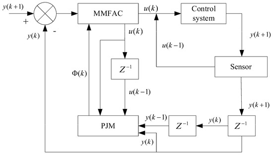
Figure 1.
System control block diagram of the MMFAC algorithm.
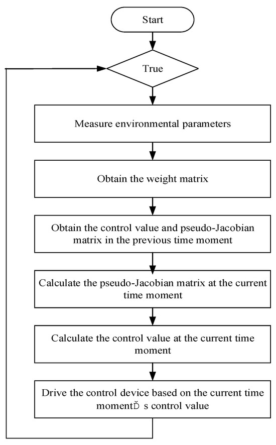
Figure 2.
Flowchart of the MMFAC algorithm.
Step 1: Environmental parameters are measured and inputted, with the measured values stored in .
Step 2: The weight matrix, the expected values of environmental parameters at the next time instant , and the control input and pseudo-Jacobian matrix (PJM) from the previous time step and are sequentially acquired.
Step 3: The current is calculated via Equation (12).
Step 4: The control input at the current time is computed by applying Equation (10).
Final Step: Devices in the data center, such as air conditioners, fans, and dehumidifiers, are regulated according to the computed control input.
Through cyclic execution of the above steps, the MMFAC algorithm enables environmental temperature control in data centers.
3. Experimental Verification
This study focuses on a data center as the subject of investigation. The layout of cabinets and terminal air conditioners in the data center is illustrated in Figure 2. To prevent server overheating, hotspots, and other issues, the data center design specifies a hot-aisle temperature range of 31 to 35 °C. In this particular data center, the cold-aisle temperature should be maintained within the range of 21 to 25 °C, with an indicated airflow volume between 2.4 and 3.9 kW·h based on power consumption over a period of 15 min.
To achieve precise control over the hot-aisle temperature in the data center, this study selects two machine cabinets (circled in red) along with two cold aisles and one hot aisle (also circled in red) as research objects, shown in Figure 3. Additionally, two air control groups (circled in blue), namely, Air Conditioning Unit 1 consisting of CRAC01 and CRAC02 units and Air Conditioning Unit 2 comprising CRAC03 and CRAC04 units, are chosen for analysis purposes. Each air conditioning group supplies cold air to its respective cold aisle. Group 1 serves Cold Aisle 1 while Group 2 caters to Cold Aisle 2.
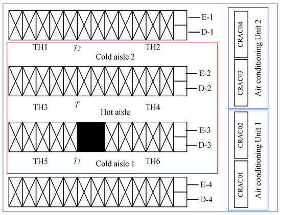
Figure 3.
Part of the plan of a data center computer room.
Within each air conditioning group, both units operate under identical conditions and modes. Temperature measuring points are present within each hot and cold aisle; specifically, TH3 and TH4 represent temperature measuring points for the hot aisle (as shown by the red box). For subsequent analysis purposes, temperature T1 of the Cold Aisle 1 is recorded.
In terms of power supply distribution within the red box depicted in Figure 3, upper-cabinet servers are powered by E-2 and D-2 power supplies while lower-cabinet servers receive power from E-3 and D-3 sources.
3.1. Establishment of Prediction Model in Data Center
The hot-aisle temperature prediction model represents the correlation among air conditioner output (cold-aisle temperature, cold-aisle air volume), server power consumption, and cabinet hot-aisle temperature.
3.1.1. Data Collection
In this study, a sampling period of 15 min was employed from 25 October in the first year to 7 March in the second year.
3.1.2. Model Input and Output Parameters
The input parameters of the model are as follows, where k represents the current moment:
1. System control quantity: Active power and and cold-aisle temperature and of Air Conditioning Unit 1 and Air Conditioning Unit 2.
2. System disturbance: E-7, D-7, E-6, and D-6 for incoming line active power , , , and .
3. System output: the temperatures of the hot aisle, cabinet TH3, and cabinet TH5, recorded as the moment vector , , and .
The model output is the temperature at the next moment, , , and .
3.1.3. Model Performance Analysis
The trained hot-aisle temperature model was utilized in this study to compare the predicted temperatures with actual field measurements, based on 200 datasets collected over a specific two-day period from the test set. As shown in Figure 4, the model’s temperature predictions align closely with the observed field data, as indicated by the root-mean-square error of 0.1328 °C. The maximum prediction error is 0.3393 °C, demonstrating a strong correspondence between the model output and target values. Consequently, the established hot-aisle temperature prediction model effectively captures variations in hot-aisle temperature resulting from changes in server power consumption and adjustments made to air conditioner settings for cabinet cooling.
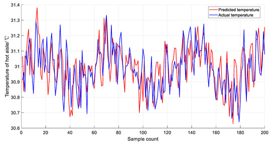
Figure 4.
Comparison between the actual temperature of hot aisles and the predicted temperature of the model.
3.2. Experimental Verification
The effectiveness of the improved algorithm is validated based on the established prediction model for hot-aisle temperature in data centers. The prediction model represents a MIMO system with four control inputs, three outputs, and four perturbations. Considering the design requirements of the data center, the desired output for hot-aisle temperature is set at 31 °C. In this study, continuous power data, supplying power to the cabinet in the data center, are utilized to simulate power consumption variations caused by changes in the computing load that on-site servers experience every 15 min.
During comparative experiments, each control method undergoes ten instances of power change testing followed by 100 control iterations after each change. Each iteration has a control interval of 9 s, resulting in a series of controlled outcomes that are analyzed for feasibility and effectiveness.
Figure 5 and Figure 6, respectively, show the output curves and absolute value error curves of the hot-aisle temperature prediction model controlled by the PID controller and the MMFAC controller. The figures indicate that compared with the MMFAC controller, the PID controller exhibits larger overshoot, slow response to partial power changes, and longer oscillation times. The experimental results show that the PID controller has poor application effects in complex MIMO systems and cannot fully adapt to the dynamic changes in the system. However, by applying the predictive function, the MMFAC controller can accurately track the desired output targets and achieve better control performance.
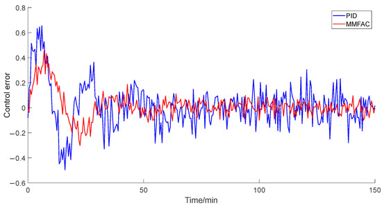
Figure 5.
Comparison of control errors between PID and MMFAC.
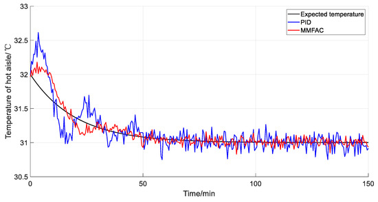
Figure 6.
Comparison of temperature of hot aisle between PID and MMFAC.
Figure 7 shows the output control quantity curves for the cold-aisle temperatures of the two air conditioning groups. It can be observed that to maintain the data center temperature at 31 °C, the energy consumption of Air Conditioning Unit 1 is consistently slightly higher than that of Unit 2. This is because Cold Aisle 1 has more server racks deployed than Cold Aisle 2, resulting in a higher cooling demand during normal data center operation. This demonstrates that the algorithm presented in this paper adaptively adjusts the cooling equipment according to actual requirements. This further reveals the reason why the MMFAC algorithm has smaller temperature control errors.
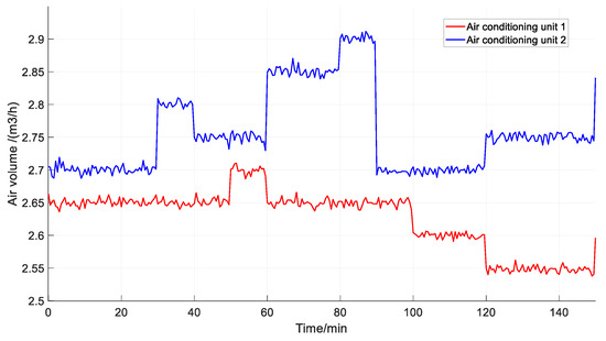
Figure 7.
Air volume control curve of MMFAC.
To achieve precise temperature control, different weight coefficients can be set for various devices and hot aisles. In this paper, the temperature control of cabinet TH3 is set as the highest priority with a weight coefficient of 10; the temperature control of cabinet TH5 is set as the secondary priority with a weight coefficient of 1; and the temperature control weight coefficient of the hot aisle is set as 0.1. The temperature control coefficients of the three elements are shown in Figure 8.
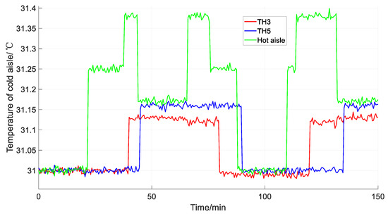
Figure 8.
Control output curve of MMFAC.
From Figure 8, it can be seen that with the load changes in each cabinet in the data center, the temperature variations in different cabinets are inconsistent. After the air conditioning units are regulated by the MMFAC algorithm, the temperature rise in cabinet TH3 is alleviated first and can be maintained at around 31 °C for a long time, followed by that of cabinet TH5 and, finally, the overall temperature of the hot aisle between cabinets. It can also be assumed from the figure that although the weight coefficient of the hot-aisle temperature control is the lowest, its maximum temperature still does not exceed 31.4 °C. It can be seen that the MMFAC algorithm can better achieve cabinet-level temperature control.
3.3. Comparison of Control Performance of Various Control Methods
The performance comparison results among the MMFAC, PID, IPSO (Improved Particle Swarm Optimization), and DQN (Deep Q-Network) are presented in Table 1. In Table 1, the overall error represents the sum of absolute errors in hot-aisle temperature over 1200 controls within 200 min. The total overshoot and total adjustment time denote the sums of hot-aisle temperature overshoot and adjustment time, respectively, for 120 power changes within 20 min during 10 control modifications.

Table 1.
Performance comparison of various controllers.
The results indicate that among the four control algorithms, the MMFAC algorithm achieves the minimum values in both overall cumulative error (40.75 °C) and total overshoot (1.57 °C).
The overall temperature control error of the DQN algorithm is nearly twice that of the MMFAC method. This phenomenon is primarily attributed to the fact that the DQN algorithm is more suitable for long-term dynamic optimization problems, requiring a large accumulation of data samples during its training process. However, due to the limited duration of this experiment (200 min), the volume of accumulated data was insufficient. In contrast, the MMFAC algorithm is capable of completing optimization calculations with a relatively small amount of sample data. In terms of overshoot control, the performance of the DQN algorithm is also slightly inferior to that of the MMFAC algorithm.
The adjustment time reflects the efficiency of each control algorithm in the process of temperature solving and regulation. The adjustment time of the PID algorithm exceeded 20 min, indicating that it failed to complete temperature regulation within the data statistical period, thus exhibiting low efficiency in temperature solving and regulation. Both the DQN and MMFAC algorithms can quickly generate adjustment commands during operation, but the DQN algorithm shows a certain lag in regulation effectiveness. This is due to the complexity of designing its reward function—improper design of the reward function tends to lead to the generation of suboptimal solutions, thereby reducing the overall temperature control effect.
The “electricity-saving ratio” in the table is defined as the percentage of electricity saved by each optimization algorithm relative to the baseline power consumption, where the baseline is the power consumption of the cabinet without optimization control. The data show that the MMFAC algorithm is expected to reduce cooling energy consumption by 25.4%, while the saving ratios of other algorithms such as the DQN decrease in sequence. These results further confirm the significant advantages of the MMFAC algorithm in both temperature control accuracy and energy-saving efficiency.
In large-scale data centers, server racks and cooling units can be partitioned into multiple cooling zones, each with customized target temperatures and constraint ranges. The MMFAC algorithm can be employed within individual zones to achieve precise temperature control, while optimization algorithms such as the DQN can be leveraged to develop collaborative cooling strategies, enabling inter-zone coordination. This hierarchical approach integrates localized MMFAC-based control with system-wide DQN-driven optimization, thereby realizing holistic temperature management and energy efficiency across the entire data center infrastructure.
4. Conclusions
Through experimental validation of the hot-aisle prediction model in data center control, this study demonstrates that the MMFAC algorithm with an introduced weight matrix can achieve precise cabinet-level temperature regulation in data centers without the need for detailed modeling of each device. Meanwhile, the MMFAC algorithm is capable of effectively determining optimal controller parameters based on the dynamic and time-varying characteristics of the system, thereby realizing accurate tracking of the expected temperature. Compared with other algorithms, it exhibits superior performance in improving system control efficiency, reducing overshoot, and minimizing control errors, which further lowers the energy consumption of data centers. Additionally, the algorithm provides certain insights into research on temperature control strategies in large-scale data centers.
Author Contributions
Conceptualization, methodology, writing—original draft preparation, and funding acquisition, D.J.; software and formal analysis, S.Z.; project administration, K.P. All authors have read and agreed to the published version of the manuscript.
Funding
This research was funded by Guangzhou Power Supply Bureau of Guangdong Power Grid Co., Ltd./award number 0301002022030102YS00002.
Data Availability Statement
Data supporting the results of this study are limited in availability. The data is obtained from third parties and may be obtained from the author with their permission.
Conflicts of Interest
Author Di Jiang was employed by the company Guangzhou Power Supply Bureau of Guangdong Power Grid Co., Ltd. The remaining authors declare that the research was conducted in the absence of any commercial or financial relationships that could be construed as a potential conflict of interest. The [company Guangdong Power Grid Co., Ltd. in affiliation and funding] had no role in the design of the study; in the collection, analyses, or interpretation of data; in the writing of the manuscript, or in the decision to publish the results.
References
- Katal, A.; Dahiya, S.; Choudhury, T. Energy efficiency in cloud computing data centers: A survey on software technologies. Clust. Comput. 2023, 26, 1845–1875. [Google Scholar] [CrossRef]
- Zhang, Y.; Shan, K.; Li, X.; Li, H.; Wang, S. Research and Technologies for next-generation high-temperature data centers–State-of-the-arts and future perspectives. Renew. Sustain. Energy Rev. 2023, 171, 112991. [Google Scholar] [CrossRef]
- Mitchell-Jackson, J.; Koomey, J.G.; Nordman, B.; Blazek, M. Data center power requirements: Measurements from Silicon Valley. Energy 2003, 28, 837–850. [Google Scholar] [CrossRef]
- Maggos, T.; Binas, V.; Panagopoulos, P.; Skliri, E.; Theodorou, K.; Nikolakopoulos, A.; Kiriakidis, G.; Giama, E.; Chantzis, G.; Papadopoulos, A. Improvement of Buildings’ Air Quality and Energy Consumption Using Air Purifying Paints. Appl. Sci. 2024, 14, 5997. [Google Scholar] [CrossRef]
- Zhang, Y.; Zhang, K.; Liu, J.; Kosonen, R.; Yuan, X. Airflow uniformity optimization for modular data center based on the constructal T-shaped underfloor air ducts. Appl. Therm. Eng. 2019, 155, 489–500. [Google Scholar] [CrossRef]
- Chu, W.-X.; Wang, R.; Hsu, P.-H.; Wang, C.-C. Assessment on rack intake flowrate uniformity of data center with cold aisle containment configuration. J. Build. Eng. 2020, 30, 101331. [Google Scholar] [CrossRef]
- Fang, Q.; Zhou, J.; Wang, S.; Wang, Y. Control-oriented modeling and optimization for the temperature and airflow management in an air-cooled data-center. Neural Comput. Appl. 2022, 34, 5225–5240. [Google Scholar] [CrossRef]
- Luo, Y.; Andresen, J.; Clarke, H.; Rajendra, M.; Maroto-Valer, M. A decision support system for waste heat recovery and energy efficiency improvement in data centres. Appl. Energy 2019, 250, 1217–1224. [Google Scholar] [CrossRef]
- Corigliano, O.; Algieri, A.; Fragiacomo, P. Turning Data Center Waste Heat into Energy: A Guide to Organic Rankine Cycle System Design and Performance Evaluation. Appl. Sci. 2024, 14, 6046. [Google Scholar] [CrossRef]
- Yao, L.; Huang, J.H. Multi-objective optimization of energy saving control for air conditioning system in data center. Energies 2019, 12, 1474. [Google Scholar] [CrossRef]
- Wang, P.; Sun, J.; Yoon, S.; Zhao, L.; Liang, R. A global optimization method for data center air conditioning water systems based on predictive optimization control. Energy 2024, 295, 130925. [Google Scholar] [CrossRef]
- Zaini, F.A.; Sulaima, M.F.; Razak, I.A.W.A.; Zulkafli, N.I.; Mokhlis, H. A Review on the Applications of PSO-Based Algorithm in Demand Side Management: Challenges and Opportunities. IEEE Access 2023, 11, 53373–53400. [Google Scholar] [CrossRef]
- Lv, L.; Wang, D.; Chen, Y.; Chen, H.; Wei, J.Q. Research on Operation Optimization of Central Air Conditioning Cold Source System Based on PSO-SA Algorithm. J. Phys. Conf. Ser. 2021, 2087, 012098. [Google Scholar] [CrossRef]
- Kardani, N.; Bardhan, A.; Kim, D.; Samui, P.; Zhou, A. Modelling the energy performance of residential buildings using advanced computational frameworks based on RVM, GMDH, ANFIS-BBO and ANFIS-IPSO. J. Build. Eng. 2021, 35, 102105. [Google Scholar] [CrossRef]
- Yang, Z.; Du, J.; Lin, Y.; Du, Z.; Xia, L.; Zhao, Q.; Guan, X. Increasing the energy efficiency of a data center based on machine learning. J. Ind. Ecol. 2022, 26, 323–335. [Google Scholar] [CrossRef]
- Sun, P.; Guo, Z.; Liu, S.; Lan, J.; Hu, Y. QOS-Aware Flow Control for Power-Efficient Data Center Networks with Deep Reinforcement Learning. In Proceedings of the ICASSP 2020–2020 IEEE International Conference on Acoustics, Speech and Signal Processing (ICASSP), Barcelona, Spain, 4–8 May 2020; pp. 3552–3556. [Google Scholar]
- Hogade, N.; Pasricha, S. Game-Theoretic Deep Reinforcement Learning to Minimize Carbon Emissions and Energy Costs for AI Inference Workloads in Geo-Distributed Data Centers. IEEE Trans. Sustain. Comput. 2024, 1–14. [Google Scholar] [CrossRef]
- Li, C.; Zhu, D.; Hu, C.; Li, X.; Nan, S.; Huang, H. ECDX: Energy consumption prediction model based on distance correlation and XGBoost for edge data center. Inf. Sci. 2023, 643, 119218. [Google Scholar] [CrossRef]
- Guo, Y.; Hou, Z.; Liu, S.; Jin, S. Data-Driven Model-Free Adaptive Predictive Control for a Class of MIMO Nonlinear Discrete-Time Systems with Stability Analysis. IEEE Access 2019, 7, 102852–102866. [Google Scholar] [CrossRef]
- Hou, Z.; Liu, S.; Tian, T. Lazy-Learning-Based Data-Driven Model-Free Adaptive Predictive Control for a Class of Discrete-Time Nonlinear Systems. IEEE Trans. Neural Netw. Learn. Syst. 2017, 28, 1914–1928. [Google Scholar] [CrossRef]
- Sanayei, S.; Nosratinia, A. Antenna selection in MIMO systems. IEEE Commun. Mag. 2004, 42, 68–73. [Google Scholar] [CrossRef]
- Hou, Z.; Lei, T. Constrained Model Free Adaptive Predictive Perimeter Control and Route Guidance for Multi-Region Urban Traffic Systems. IEEE Trans. Intell. Transp. Syst. 2022, 23, 912–924. [Google Scholar] [CrossRef]
- Li, D.; De Schutter, B. Distributed Model-Free Adaptive Predictive Control for Urban Traffic Networks. IEEE Trans. Control Syst. Technol. 2022, 30, 180–192. [Google Scholar] [CrossRef]
- Zhou, P.; Zhang, S.; Wen, L.; Fu, J.; Chai, T.; Wang, H. Kalman Filter-Based Data-Driven Robust Model-Free Adaptive Predictive Control of a Complicated Industrial Process. IEEE Trans. Autom. Sci. Eng. 2022, 19, 788–803. [Google Scholar] [CrossRef]
- Wang, S.; Li, J.; Hou, Z.; Meng, Q.; Li, M. Composite Model-free Adaptive Predictive Control for Wind Power Generation Based on Full Wind Speed. CSEE J. Power Energy Syst. 2022, 8, 1659–1669. [Google Scholar]
- Lei, T.; Hou, Z. Perimeter control for two-region urban traffic system based on model free adaptive predictive control with constraints. IFAC PapersOnLine 2019, 52, 25–30. [Google Scholar] [CrossRef]
Disclaimer/Publisher’s Note: The statements, opinions and data contained in all publications are solely those of the individual author(s) and contributor(s) and not of MDPI and/or the editor(s). MDPI and/or the editor(s) disclaim responsibility for any injury to people or property resulting from any ideas, methods, instructions or products referred to in the content. |
© 2025 by the authors. Licensee MDPI, Basel, Switzerland. This article is an open access article distributed under the terms and conditions of the Creative Commons Attribution (CC BY) license (https://creativecommons.org/licenses/by/4.0/).