Physics-Constrained Diffusion-Based Scenario Expansion Method for Power System Transient Stability Assessment

Abstract

In transient stability assessment (TSA) of power systems, the extreme scarcity of unstable scenario samples often leads to misjudgments of fault risks by assessment models, and this issue is particularly pronounced in new-type power systems with high penetration of renewable energy sources. To address this, this paper proposes a physics-constrained diffusion-based scenario expansion method. It constructs a hierarchical conditional diffusion framework embedded with transient differential equations, combines a spatiotemporal decoupling analysis mechanism to capture grid topological and temporal features, and introduces a transient energy function as a stability boundary constraint to ensure the physical rationality of generated scenarios. Verification on the modified IEEE-39 bus system with a high proportion of new energy sources shows that the proposed method achieves an unstable scenario recognition rate of 98.77%, which is 3.92 and 2.65 percentage points higher than that of the Synthetic Minority Oversampling Technique (SMOTE, 94.85%) and Generative Adversarial Networks (GANs, 96.12%) respectively. The geometric mean achieves 99.33%, significantly enhancing the accuracy and reliability of TSA, and providing sufficient technical support for identifying the dynamic security boundaries of power systems.

1. Introduction

With the massive integration of new energy sources and power electronic devices in the receiving-end provincial new power system [1,2], the continuous expansion of grid scale [3], and the increasing complexity of operation conditions, transient stability assessment (TSA) of power systems, as a core means to identify the dynamic safety boundaries of the system and ensure the resilient operation of the power grid, is crucial for preventing cascading failures and maintaining the balance of power supply and demand in terms of its accuracy and timeliness [4,5,6]. However, clarifying the transient stability characteristics of the system under different new energy penetration rates, which is the basic logic for TSA to determine the stability support demand, is facing severe challenges due to the coupling of multi-energy subjects and the dynamic variation in operating conditions [7]. Traditional TSA methods, such as the time-domain simulation method [8] and the direct method [9], struggle to balance high assessment accuracy and efficient speed requirements for complex power grids [10]. Against this backdrop, the integration scheme of massive dynamic data from synchronized phasor measurement units (PMUs) and intelligent analysis techniques [11] provides a new pathway for constructing data-driven intelligent assessment paradigms. By establishing nonlinear mappings between fault feature quantities and system stability states, this approach enables effective and rapid identification of transient stability postures [12].

TSA in power systems confronts a typical class imbalance challenge: stable operation conditions dominate in practical operation, leading to extreme sparsity of transient unstable scenarios [13]. Such distribution skewness efficiently induces majority-class preference bias in assessment models, manifesting as inflated global classification metrics and significantly degraded capability for unstable scenarios. Notably, although transient instability events have a low occurrence probability, misjudging them can trigger severe cascading failures, underscoring the critical need for early warnings to enhance models’ sensitivity to tail risks. Current research integrates cost-sensitive learning with feature space reconstruction strategies to effectively mitigate model discrimination distortion caused by inter-class scenario magnitude differences, offering an important technical pathway to improve assessment system reliability. In the realm of TSA, a pioneering data-driven approach [14] integrates an “aggressive-conservative” support vector machine architecture, strategically enhancing the interpretability of TSA outcomes while mitigating the risks of false alarms and omissions. Another notable contribution [15] introduces a sophisticated fusion of graph convolutional networks (GCNs) and long short-term memory (LSTM) networks, enabling in-depth analysis of transient angle stability by decoding spatiotemporal disturbance signatures in future power systems with increased new energy penetration. For AC/DC hybrid power grids, an innovative TSA framework [16] has been developed, leveraging autoencoder-based feature extraction coupled with Boltzmann machine training to ensure both accuracy and robustness in stability evaluation.

In recent years, the sustainability assessment of transient processes has emerged as a pivotal focus in energy systems, focusing on quantifying a system’s ability to sustain stable operations during transients and analyzing the controllability of fault evolution. Within high-renewable-energy power systems, critical limitations persist: as highlighted in [17], wind power’s volatility amplifies transient uncertainty, rendering traditional deterministic assessment frameworks ineffective; studies on cascading failures in high-photovoltaic grids [18] further reveal that low inverter inertia and inadequate fault ride-through capability are primary culprits, yet existing TSA methodologies cannot quantify these intricate correlations. Concurrently, the virtual synchronous generator (VSG) concept—implemented in renewable energy inverter converters—has advanced substantially as a key mitigation strategy for stability challenges. By emulating the inertia and damping characteristics of synchronous generators, VSG significantly enhances transient support capabilities in new-energy-integrated systems. Notably, [19] verifies that VSG improves angle stability margins in high-wind-penetration scenarios, while [20] further illustrates that VSG’s virtual inertia regulation effectively mitigates voltage transients. However, existing scenario expansion methods remain deficient in capturing VSG-induced dynamics, creating a critical gap in modeling such enhanced systems.

While the above methods have made substantial improvements in assessment models, they overlook improvements in scenario data. The Synthetic Minority Oversampling Technique (SMOTE) [21], a linear interpolation method, can enhance the stability of datasets to some extent; however, it fails to fit real-world power system scenarios accurately and is typically limited to classical machine learning models. A scenario expansion method for power system TSA based on Generative Adversarial Networks (GANs) was proposed in [22]. This approach improves the model’s learning capability for unstable scenario distributions by adjusting the input scenario composition ratio. It promotes training convergence through a pre-training approach to provide an optimal initial state. However, although GANs can learn data distributions, they lack the embedding of power system differential-algebraic equation constraints, leading to the generation of unstable scenarios that deviate from the physical laws of dynamic processes and pose risks of “data hallucination”. These limitations highlight a critical gap: existing data-driven scenario expansion methods either rely on simplistic linear interpolation or generate physically implausible samples due to the absence of domain-specific constraints, hindering their effectiveness in TSA.

To address this gap and specifically tackle the insufficient adaptability of existing scenario generation methods to physical rules in power system TSA, this paper proposes a Physics-Constrained Diffusion–Self-Attention Coupling (PCDiff-TSA)-based scenario expansion method, whose core architecture and innovations are as follows:

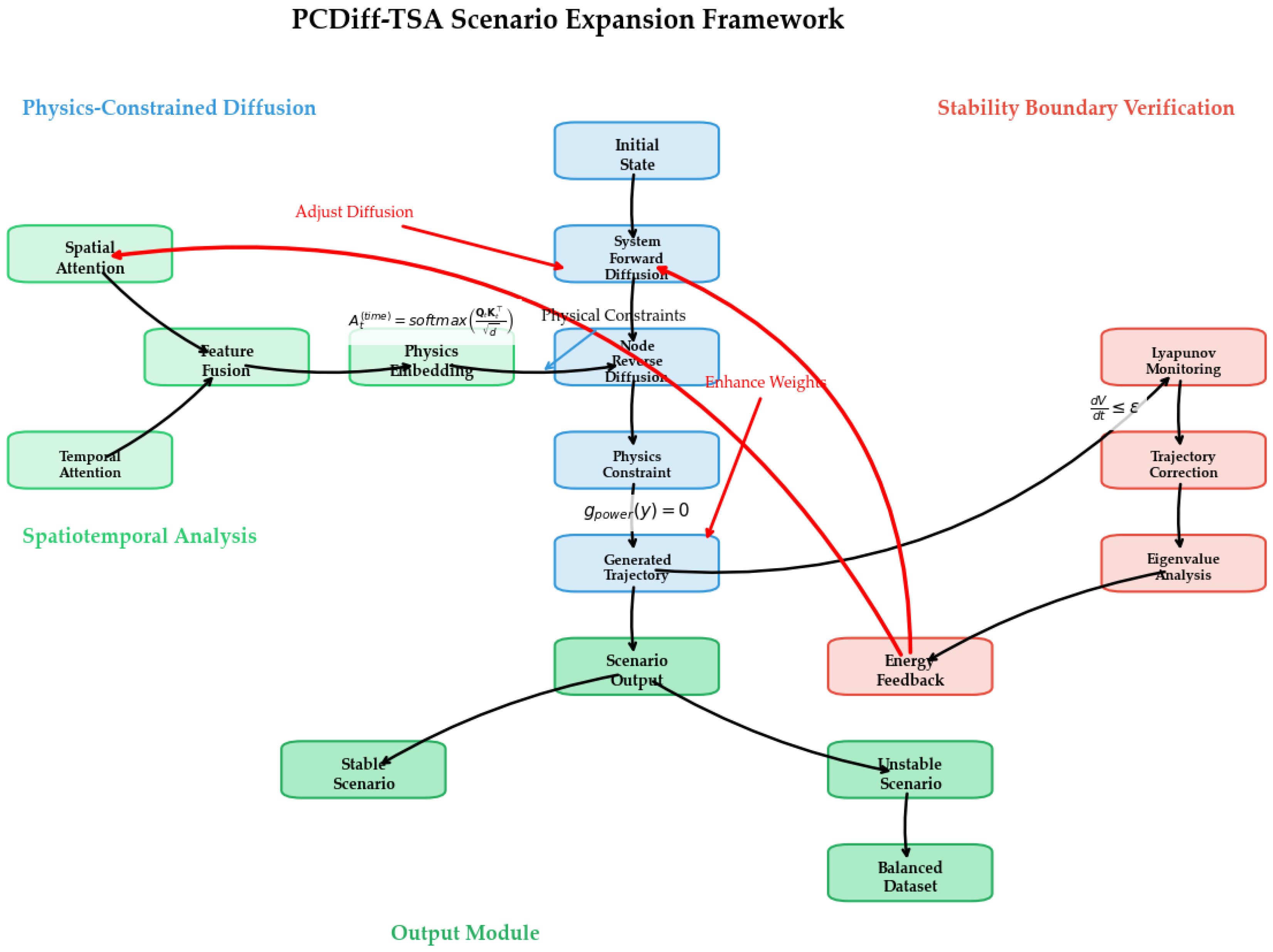
• A Physics-Constrained Hierarchical Conditional Diffusion Framework: This framework embeds transient differential equation constraints into the reverse sampling process. By leveraging non-equilibrium thermodynamic sampling strategies, it achieves precise control over the physical rationality of dynamic trajectories, ensuring that the generated transient scenario trajectories strictly adhere to rotor angle motion equations and power flow balance laws, thus resolving the “data hallucination” issue caused by the lack of physical constraints in methods like GANs.
• A Spatiotemporal Decoupling Analysis Mechanism: This mechanism integrates impedance matrix regularization and power-angle swing feature decoupling modules. It separately captures grid topological correlation characteristics (via spatial analysis) and time-series oscillation patterns (via temporal analysis), addressing the inability of linear methods like SMOTE to model complex nonlinear spatiotemporal dynamics in power systems.
• A Stability Boundary-Aware Verification Mechanism: By introducing a transient energy function as stability boundary-aware loss and combining it with the Lyapunov direct method, this mechanism constructs a dynamic verification loop. It ensures that the generated scenarios comply with actual system safety thresholds, enhancing the reliability of scenario expansion for TSA.

The remaining sections are organized as follows: Section 2 describes the basic principles of PCDiff-TSA. Section 3 introduces the transient stability scenario enhancement model based on PCDiff-TSA. Section 4 presents simulation analyses on the modified IEEE 39-bus system. Section 5 concludes the paper and outlines future prospects.

2. Materials and Methods

The PCDiff-TSA model is a physics-constrained diffusion-based scenario expansion framework designed for power system transient stability assessment. It integrates non-equilibrium thermodynamic sampling with power system dynamic equations, embedding transient differential constraints into the reverse diffusion process. Through a spatiotemporal decoupling attention mechanism, it captures grid topological correlations and time-series oscillation patterns, while introducing transient energy functions and Lyapunov stability criteria as boundary constraints. This model ensures that the generated scenarios strictly adhere to physical laws and enhances the diversity and authenticity of unstable scenarios, thereby improving the accuracy of transient stability assessment models. The flowchart of the PCDiff-TSA model is shown in Figure 1.

2.1. PCDiff Model Basics

The physically constrained diffusion model proposed in this paper integrates a non-equilibrium thermodynamic sampling framework with the dynamic equations of the power system. Its core lies in the fact that the forward diffusion process will gradually inject dynamic noise with the help of stochastic differential equations. In contrast, the reverse process restores the system trajectory under the constraints of physical laws. The mathematical description of the forward process is

$$d{x}_t=f_{\mathrm{phys}}\left(x_t,t\right)dt+\sqrt{\beta \left(t\right)}d{W}_t$$

(1)

where f_phys(x_t, t) is constructed from the rotor motion equation, and its specific form is

$$f_{\mathrm{phys}}={\displaystyle \frac{d\delta }{dt}}-\left(\omega -{\omega }_0\right)+{\displaystyle \frac{1}{2M}}\left(P_m-P_e\right)$$

(2)

where δ is the power angle of the generator, M is the inertia constant of the unit, β(t) is the noise intensity attenuation control function over time, and W_t represents the increment of the Wiener process.

The reverse generation process embeds physical constraints in the denoising stage. By modifying the evolution direction of the stochastic differential equation, it forces the trajectory to satisfy the dynamic laws of the power system. Its mathematical description is

$$d{x}_{t-1}=\left[f_{\mathrm{phys}}\left(x_t,t\right)-{\displaystyle \frac{\beta \left(t\right)}{2}}{\nabla }_x\log p_t\left(x\right)\right]dt+\sqrt{\beta \left(t\right)}d{W}_t$$

(3)

where ${\nabla }_x\log p_t\left(x\right)$ is the score function, which is approximated by neural network learning.

Meanwhile, to ensure strict compliance with physical laws, a physical equation residual constraint is introduced:

$$L_{\mathrm{phys}}=\mathsf{{\rm E}}{‖{\displaystyle \frac{\partial x}{\partial t}}-f_{\mathrm{phys}}\left(x,t\right)‖}^2$$

(4)

This model utilizes the physical equation as a hard constraint through variational inference, ensuring that the generated trajectory satisfies the conditions of energy conservation and power-angle stability. Compared with traditional diffusion models [23], the introduction of physical constraints can compress the trajectory sampling space to the solution space of the differential equation. While improving the generation efficiency, it ensures the physical rationality of the trajectory. The noise injection process retains the modeling ability for the dynamic uncertainty of the power system, allowing the model to adapt to the simulation requirements of complex operating scenarios.

2.2. Embedding Mechanism of Power System Transient Differential Equations

The embedding mechanism [24] of power system transient differential equations aims to guide the scenario generation process of the generative model through the rigid constraints of differential-algebraic equations, ensuring that the synthesized data strictly conforms to the dynamic characteristic laws of the power system. This mechanism utilizes the classic second-order rotor motion equation as the core constraint to construct dual guarantees of physical consistency and dynamic stability.

2.2.1. Core Dynamic Constraints: Second-Order Rotor Motion Equation

In a power system, the transient characteristics of a synchronous generator are described by the second-order rotor motion equation [25], and its form is

$$\left\{\begin{array}{l}{\displaystyle \frac{d{\delta }_i}{dt}}={\omega }_i-{\omega }_0\\ M_i {\displaystyle \frac{d{\omega }_i}{dt}}=P_{m,i}-P_{e,i}-D_i\left({\omega }_i-{\omega }_0\right)\end{array}\right.$$

(5)

where δ_i and ω_i are the power angle and angular velocity of the generator, respectively; ω₀ is the synchronous angular velocity; M_i and D_i are the inertia constant and damping coefficient of the unit, respectively; and P_m,i and P_e,i are the mechanical power and electromagnetic power of the unit, respectively.

2.2.2. Residual-Driven Loss Function

To embed the above-mentioned dynamic equation into the generative model, a variational inference framework is adopted, and the equation residual is introduced into the loss function as a constraint term. Its form is

$$L_{\mathrm{DAE}}={\lambda }_1\mathsf{{\rm E}}{‖{\displaystyle \frac{d\widehat{x}}{dt}}-f_{\mathrm{swing}}\left(\widehat{x}\right)‖}_2+{\lambda }_2\mathsf{{\rm E}}{‖g\left(\widehat{x},y\right)‖}_2$$

(6)

where $\widehat{x}$ is the transient trajectory output by the generative model, $f_{\mathrm{swing}}\left(\widehat{x}\right)$ is the right-hand-side term of (5), $g\left(\widehat{x},y\right)$ is the algebraic constraint for node power balance, and ${\lambda }_1$ and ${\lambda }_2$ are the weight coefficients of the constraint terms, which are used to balance the influence of the dynamic equation and the algebraic constraint.

2.2.3. Regularization of Transient Energy Function

To further ensure the transient stability of the generated scenarios [26], a transient energy function is introduced as a regular term, and its definition is

$$V\left(\delta ,\omega \right)={\displaystyle \frac{1}{2}}{\displaystyle \sum M_i{\left({\omega }_i-{\omega }_0\right)}^2}-{\displaystyle \sum P_{m,i}\left({\delta }_i-{\delta }_i^s\right)+{\displaystyle \sum C_{ij}\left(1-\cos \left({\delta }_i-{\delta }_j\right)\right)}}$$

(7)

where ${\delta }_i^s$ is the steady-state power angle before the fault, while C_ij is the transient energy coefficient of line ij. The physical meanings of this function are as follows: the first term is the kinetic energy related to the angular velocity deviation, the second term is the potential energy change determined by the mechanical power and power-angle deviation, and the third term is the network coupling potential energy characterized by the cosine of the power-angle difference between units.

During the generation process, by forcibly satisfying the dissipative condition of the energy function,

$${\displaystyle \frac{dV}{dt}}=-{\displaystyle \sum D_i{\left({\omega }_i-{\omega }_0\right)}^2\le 0}$$

(8)

The role of the dissipative condition is to ensure that the generated trajectory is always within the stable region—the energy function decreases monotonically with time. Finally, it converges to the steady state, thus avoiding the generation of unstable trajectories.

In summary, the embedding mechanism of power system transient differential equations achieves three objectives through “hard constraints of dynamic equations and regularization of stability”:

• Force scenarios to satisfy the dynamic laws of the power system and avoid physical irrationality problems;
• Rely on the dissipativity of the transient energy function to ensure that the trajectory is in the stable region, adapting to TSA;
• Explicitly embed physical equations, endow the generation process with mechanism support, and make up for the black-box defect of pure data-driven models.

It should be noted that the current physical constraints primarily focus on generator rotor angle dynamics to ensure the transient stability of the angle. For voltage stability—particularly the voltage sensitivity of motor loads in industrial settings—the constraint system can be further expanded: a voltage deviation term can be introduced into the transient energy function, and induction motor dynamic models can be embedded. This allows the generated scenarios to reflect the coordinated evolution of both rotor angle and voltage, providing more comprehensive stability assessment support for systems with high proportions of industrial loads.

2.3. Spatiotemporal Decoupling and Self-Attention Coupling

Given the spatiotemporal correlation characteristics of the dynamic trajectories in power systems, a decoupled attention mechanism is designed to capture such complex correlation information more accurately and efficiently.

2.3.1. Spatiotemporal Decoupling Attention Decomposition

The spatiotemporal decoupling strategy decomposes the standard attention matrix into time–space dual channels, focusing on modeling the temporal dynamics and spatial correlations, respectively.

(1)

Temporal Self-Attention

This is used to mine the evolution laws and dependency relationships of the power system states in the time dimension. The formula is

$$A_{ij}^T=\mathrm{softmax}\left({\displaystyle \frac{Q_{x_i}{K}_{x_i}^{\mathrm{T}}}{\sqrt{d}}}\right),\forall i,j\in {\tau }_{\mathrm{seq}}$$

(9)

where $Q_{x_i}$ are $K_{x_i}$ the query and key vectors in the time dimension, respectively, ${\tau }_{\mathrm{seq}}$ represents the time window, and d is the feature dimension. The temporal attention weights are obtained through softmax normalization, depicting the correlation intensity between states at different moments.

(2)

Spatial Self-Attention

This focuses on capturing the spatial coupling characteristics between nodes in the power grid. The formula is

$$A_{mn}^S=\mathrm{softmax}\left({\displaystyle \frac{\left(Q_{y_m}+\varphi b_{mn}\right)K_{y_n}^{\mathrm{T}}}{\sqrt{d}}}\right),\forall m,n\in N$$

(10)

where $Q_{y_m}$ and $K_{y_n}$ are the query and key vectors in the spatial dimension, respectively, N is the set of nodes, $\varphi \left(b_{mn}\right)=\exp \left(-{\gamma }_{mn}\cdot \mathsf{\Delta }t\right)$ is the node electrical distance encoding, ${\gamma }_{mn}$ is taken from the elements of the admittance matrix, and $\mathsf{\Delta }t$ is the time interval. Through this encoding, the electrical distance information between nodes is integrated into the spatial attention calculation, enabling the spatial attention to reflect the influence of network topology and electrical characteristics on node correlations.

2.3.2. Physical Constraint Coupling Interaction

To deeply integrate the attention mechanism with the physical laws of the power system, an interaction relationship is established through dynamic equations. The formula is

$$h_{\mathrm{fusion}}=\sigma \left(W\cdot \left[A^T\otimes {\displaystyle \frac{\partial f_{\mathrm{swing}}}{\partial x}};A^S\otimes {\displaystyle \frac{\partial g_{\mathrm{power}}}{\partial y}}\right]\right)$$

(11)

where g_power is the node power balance equation, constraining the power supply–demand relationship of the power system. W is the weight matrix, and $\sigma$ is the activation function. This design makes the attention weights have a dynamic correlation with the system’s Jacobian matrix, enabling the attention mechanism to follow the physical constraints of the power system during the learning process, and improving the model’s ability to model the characteristics of the power system.

2.4. Construction of Physics-Constrained Generative Model

2.4.1. Hybrid Conditional Encoding Strategy

In the scenario of power system transient stability analysis, it is necessary to handle continuous operation states and discrete topology constraints simultaneously. To achieve the unified encoding of these two types of heterogeneous conditions, a dual-channel conditional encoder is designed to perform feature extraction on the operation states and topology structures, respectively, and then realize information interaction through a dynamic fusion mechanism.

(1)

Operation State Encoding

For the continuous operation states of the power system, the Fourier feature projection method is adopted for encoding to mine the nonlinear correlations among continuous variables. The formula is

$$z_{\mathrm{op}}=W_{\gamma }\cdot \cos \left(2\pi \gamma \odot \left[V,\delta ,\omega \right]\right)+b_{\gamma }$$

(12)

where $\gamma \in {ℝ}^F$ are learnable frequency-domain parameters, and F is the frequency-domain dimension. By learning different frequency components, the complex nonlinear coupling relationships among voltage, power angle, and speed are captured. $W_{\gamma }$ and $b_{\gamma }$ are the weight matrix and bias term of the encoder, respectively.

(2)

Topology Structure Encoding

The topology structure of the power system is determined by discrete information such as the admittance of network branches and the states of circuit breakers. The graph attention mechanism is used to encode topology features. The formula is

$$\begin{array}{l}{z}_{\mathrm{topo}}^{\left(i\right)}={\displaystyle \sum _{j\in N_i}{\alpha }_{ij}\cdot \mathrm{MLP}\left(\left[Y_{ij},b_{ij}\right]\right)},\\ {\alpha }_{ij}=\mathrm{softmax}\left({\displaystyle \frac{Q_{y_i}\cdot K_{y_i}}{\sqrt{d}}}\right)\end{array}$$

(13)

where $z_{\mathrm{topo}}^{\left(i\right)}$ is the topology encoding feature of the i-th node; N_i is the neighbor set of node i; Y_ij is the admittance of branch ij; b_ij is the state of the branch circuit breaker; MLP( ) is a multi-layer perceptron, used to extract the high-dimensional features of branch information; ${\alpha }_{ij}$ is the attention coefficient learned by the graph attention mechanism, explicitly representing the electrical coupling intensity between node i and neighbor j; and $Q_{y_i}\cdot K_{y_i}$ are the query and key vectors of nodes i and j, respectively.

(3)

Dynamic Gating Mechanism

To realize the dynamic fusion of operation state encoding and topology structure encoding, a gating mechanism is designed to adaptively adjust the fusion weights of the two types of features. The formula is

$$z_{\mathrm{cond}}=\sigma \left(W_g\left[z_{\mathrm{op}};z_{\mathrm{topo}}\right]\right)\odot z_{\mathrm{op}}+\left(1-\sigma \left(W_g\left[z_{\mathrm{op}};z_{\mathrm{topo}}\right]\right)\right)\odot z_{\mathrm{topo}}$$

(14)

where $W_g$ is the weight matrix of the gating mechanism, and [z_op; z_topo] represents the feature concatenation of operation state encoding and topology structure encoding.

Additionally, the weight adjustment of the gating mechanism is adaptive, based on the gradient $\nabla V$ of the transient energy function $V\left(\delta ,\omega \right)$. When the transient energy of the system changes drastically, the weight of the topology structure encoding is increased to strengthen the influence of the network topology on transient characteristics. When the system tends toward a steady state, the operation state encoding is emphasized to focus on the evolution laws of continuous variables.

(4)

Injection of Physical Constraints

To ensure that the generated scenarios strictly satisfy the power system’s node power balance equations, physical constraints are introduced through conditional projection using the Jacobian matrix. This operation orthogonally maps the encoded features to the subspace that satisfies the node power balance equations, ensuring that the coupling relationship between the topological structure and the operating state in the generated scenarios conforms to the physical laws of power systems. This provides a strict constraint foundation for the subsequent diffusion process. The formula is

$$\widehat{z}=z_{\mathrm{cond}}-J_g^{\mathrm{T}}{\left(J_g{J}_g^{\mathrm{T}}\right)}^{-1}{J}_g{z}_{\mathrm{cond}},J_g={\displaystyle \frac{\partial g_{\mathrm{power}}}{\partial y}}$$

(15)

where J_g is the Jacobian matrix of the node power balance equation, while the Gram matrix $J_g{J}_g^{\mathrm{T}}$ quantifies the inter-product relationships between physical constraints in the encoded feature space, characterizing the correlation and coupling strength among different constraint conditions. The introduction of its inverse matrix essentially involves solving the Moore–Penrose pseudoinverse of the constraint equations, which determines the optimal direction that minimizes the feature projection error while satisfying physical constraints, such as node power balance. This ensures that when encoded features are mapped to the physically feasible domain, they not only strictly conform to power grid operation laws but also retain as much key information as possible from the original features. Through the physical constraint injection operation, the orthogonal projection maps the encoded feature $z_{\mathrm{cond}}$ to the subspace that satisfies the node power balance constraint, ensuring that the generated scenarios strictly conform to the physical laws of the power system.

2.4.2. Hierarchical Diffusion Generation Process

Aiming at the multi-timescale dynamic characteristics of the power system, a hierarchical diffusion process is designed to decouple the generation process, which specifically includes the following links:

(1)

System-Level Diffusion

Based on the hybrid conditional encoding $z_{\mathrm{cond}}$, forward diffusion is performed on the global state $x={\left[\delta ,\omega \right]}^{\mathrm{T}}$:

$$q\left(x_t\left|x_{t-1}\right.\right)=N\left(x_t;\sqrt{1-{\beta }_t}{x}_{t-1},{\beta }_{t}I\right)$$

(16)

where ${\beta }_t$ is regulated by the gradient ${‖\nabla V‖}_2$ of the Lyapunov function V(x), so that the diffusion process adapts to the evolution laws of the system’s transient stability.

(2)

Node-Level Reverse Diffusion

The local variable y = [V,P,Q]^T is corrected through the reverse process of physical constraints, and the conditional probability distribution is defined as follows:

$$p_{\theta }\left(y_{t-1}\left|y_t,z_{\mathrm{cond}}\right.\right)=N\left(y_{t-1};{\mu }_{\theta }\left(y_t,t,z_{\mathrm{cond}}\right)\right)$$

(17)

The generator ${\mu }_{\theta }$ embeds the spatiotemporal decoupling attention mechanism and injects dynamic equation constraints at each step, and it ensures physical consistency through an optimization problem:

$$\underset{\theta }{\min }{‖J_g{\displaystyle \frac{\partial g_{power}}{\partial y}}‖}_F^2,J_g=\left[\partial P/\partial V,\partial Q/\partial \delta \right]$$

(18)

(3)

Dynamic Projection Layer

Perform a physical feasibility projection every 5 iterations to enforce node power balance:

$$\widehat{y}\leftarrow y-J_g^{\mathrm{T}}{\left(J_g{J}_g^{\mathrm{T}}\right)}^{-1}{g}_{\mathrm{power}}\left(y\right)$$

(19)

This operation ensures g_power(y) = 0, forming a closed loop with the physical constraint injection in Equation (15) to guarantee the physical rationality of the generated scenarios.

2.4.3. Stability Verification Mechanism

To ensure that the electrical dynamic trajectories output by the generative model meet the transient stability requirements, a multi-level verification framework is designed, forming a closed loop with the hierarchical diffusion process.

(1)

Lyapunov Real-Time Monitoring

In power system transient stability analysis, constructing an energy function based on system dynamic equations is a key method. For multi-machine power systems, the following Lyapunov energy function is constructed:

$$V(x)={\displaystyle \frac{1}{2}}{\omega }^{\mathrm{T}}M\omega +{\displaystyle {\int }_{{\delta }_0}^{\delta }(P_m-P_e)d\delta }$$

(20)

To analyze the system’s transient stability, the time derivative of the energy function along the trajectory needs to be calculated:

$${\displaystyle \frac{dV}{dt}}={\omega }^{\mathrm{T}}(P_m-P_e-D\omega )-{\displaystyle \sum _{i=1}^n\frac{\partial V}{\partial V_i}}\left({\displaystyle \frac{d{V}_i}{dt}}\right)$$

(21)

where D is the damping matrix, and V_i is the sub-energy function quantity of the i-th generator.

To avoid transient instability, an energy derivative threshold ε (taken as 0.05 p.u.) is set. When (dV\dt > ε), a gradient stop mechanism is triggered to force correction of the generated scenario, suppressing the evolution of the system towards an unstable trajectory, and ensuring that the simulation process conforms to the actual stability boundary.

(2)

Eigenvalue Online Correction Strategy

To accurately capture the system’s transient characteristics, fast QR decomposition is performed on the Jacobian matrix $J_{\mathrm{sys}}=\partial f/\partial x$ of the generated trajectory. If the real part of the dominant mode satisfies Re(λ_max) > −0.5 (corresponding to a damping ratio < 5%, where the system exhibits weak damping or negative damping characteristics), the state quantity is corrected through physical constraint projection:

$$\widehat{x}\leftarrow x-\eta J_{\mathrm{sys}}^{\mathrm{T}}{\left(J_{\mathrm{sys}}{J}_{\mathrm{sys}}^{\mathrm{T}}\right)}^{-1}{f}_{\mathrm{swing}}\left(x\right)$$

(22)

where η is the correction step size. To ensure the physical rationality of the generator’ power angle, an additional angle constraint is added: the power-angle difference between any two generators is maintained within |δ_i − δ_j| < 120°, avoiding cascading disconnection caused by excessive power-angle differences, and ensuring that the simulation trajectory is always within the physically feasible domain, improving the accuracy and reliability of transient simulation.

(3)

Energy Margin Adaptive Adjustment Strategy

To comprehensively optimize the system’s transient stability margin and achieve dynamic regulation, an energy margin adaptive adjustment mechanism based on hybrid conditional encoding is proposed. This mechanism takes the transient energy margin as the core indicator, dynamically optimizing the system’s fault ride-through capability by fusing topology encoding and attention mechanisms.

Define the transient energy margin η_energy as the relative difference between the system’s critical energy and the current energy, and its calculation formula is

$${\eta }_{\mathrm{energy}}={\displaystyle \frac{V_{\mathrm{crit}}-V_{\mathrm{gen}}}{V_{\mathrm{gen}}}}\times 100\%$$

(23)

where V_gen is the current transient energy of the system, while V_crit is the critical energy. This indicator directly reflects the system’s remaining stability margin: the larger the value, the stronger the system’s anti-disturbance capability; the smaller the value, the closer the system is to the instability boundary. When η_energy < 15, the system is in a low-energy margin state (close to the stability boundary). At this time, the spatial attention weight is enhanced through topology encoding, and the specific implementation is as follows:

• Topology Encoding: Extract power network topology features, construct a topology adjacency matrix, and embed it into the state space.
• Attention Mechanism Optimization: In the deep learning or model prediction framework, dynamically enhance the attention weights of key nodes, and prioritize regulation of components with significant impacts on the stability margin.
• Fault Ride-Through Capability Improvement: Through the above adjustments, guide control strategies or system models to focus on high-risk areas, optimize control variable allocation, enhance the system’s fault ride-through capability under low-stability-margin conditions, and avoid cascading losses caused by minor disturbances.

2.5. Data Preprocessing and Model Evaluation Metrics

2.5.1. Spatiotemporal Alignment and Normalization

Perform time synchronization and physical dimension unification operations on the original measurement data {V_i, δ_i, P_ij, Q_ij}.

(1)

Time Synchronization

Align PMU and SCADA data through dynamic time warping (DTW), a nonlinear time-series alignment technique that optimally matches time-stamped measurements by minimizing the Euclidean distance between sequences. This addresses the inherent sampling rate discrepancies between high-frequency PMU data and low-frequency SCADA data, ensuring temporal consistency crucial for accurate transient stability analysis.

(2)

Normalization

Neural networks usually require normalization of input data before training. The formula for scenario normalization is

$$x_{pq}^{*}={\displaystyle \frac{x_{pq}-{\overline{x}}_{pq}}{\underset{p}{\max }\left(x_{pq}\right)-\underset{p}{\min }\left(x_{pq}\right)}}$$

(24)

where x_pq is the q-th feature of the p-th scenario, and ${\overline{x}}_{pq}$ is the feature mean value of the p-th scenario. After normalization, the data range is transformed to [−1, 1] for model training of scenario expansion.

2.5.2. Physical Constraint Correction

To ensure that the normalized data strictly satisfy the physical laws of the power system, a power flow equation projection constraint mechanism is introduced. For the normalized system state variable ${\widehat{D}}^{\prime }$, the following projection transformation is applied:

$${\widehat{D}}^{\prime }\leftarrow D^{\prime }-J_{\mathrm{g}}^{\mathrm{T}}{\left(J_{\mathrm{g}}{J}_{\mathrm{g}}^{\mathrm{T}}+\lambda I\right)}^{-1}{S}_{\mathrm{power}}\left(D^{\prime }\right)$$

(25)

where $S_{\mathrm{power}}\left(D^{\prime }\right)$ is the power flow equation’s residual vector, representing the deviation degree between the current state and the power flow constraint.

2.5.3. Dynamic Trajectory Decomposition

To accurately extract multi-scale dynamic features in the transient process, Fourier-wavelet hybrid transform is used for trajectory decomposition. Define the feature extraction formula of the hybrid transform as follows:

$$F\left(f\right)={\displaystyle \sum _{k=1}^K〈f,{\psi }_k\left(t\right)e^{j2\pi f_{k}t}〉}$$

(26)

where ${\psi }_k\left(t\right)$ is the wavelet basis function, which has good time–frequency localization characteristics and can capture the rapidly changing components in the transient process; $e^{j2\pi f_{k}t}$ is the Fourier complex exponent base, used to extract periodic and slowly changing components; the time-varying frequency f_kt is adaptively adjusted by the gradient of the Lyapunov energy function to realize dynamic optimization of time–frequency resolution.

2.5.4. Physical Rationality Index System

(1)

Static Rationality

Define the node power balance error index E_power to measure the satisfaction degree of the power flow constraints:

$$E_{\mathrm{power}}={\displaystyle \frac{1}{N}}{{\displaystyle \sum _{i=1}^N‖P_i-\mathrm{Re}\left(v_i{\displaystyle \sum _j{Y}_{ij}{v}_j^{*}}\right)‖}}_2$$

(27)

The smaller this index, the higher the satisfaction degree of the power flow constraints.

(2)

Dynamic Rationality

Define the transient energy error index E_energy to quantify the deviation between the Lyapunov energy function and the actual trajectory:

$$E_{\mathrm{energy}}={\displaystyle {\int }_{t_0}^{t_f}{\left(\frac{dV}{dt}-{\omega }^{\mathrm{T}}\left(P_m-P_e\right)\right)}^{2}dt}$$

(28)

This index reflects the fitting degree of the energy function to the transient process. The smaller the value, the more accurate the characterization of dynamic characteristics.

(3)

Structural Rationality

Define the condition number κ(J_g) of the Jacobian matrix J_g to evaluate the numerical stability of the power flow equation:

$$\kappa \left(J_{\mathrm{g}}\right)={\displaystyle \frac{{\sigma }_{\max }(J_g)}{{\sigma }_{\min }(J_g)}}\le {10}^6$$

(29)

where ${\sigma }_{\max }$ and ${\sigma }_{\min }$ are the maximum and minimum singular values of the Jacobian matrix, respectively. The smaller the condition number, the higher the numerical stability of matrix inversion, and the more unique and reliable the power flow solution of the corresponding power system.

2.5.5. Evaluation Metrics

To measure the model performance under scenario imbalance, a confusion matrix is introduced. It divides all instances into four groups: N_TS, N_FS, N_FU, and N_TU. The overall accuracy (A_cc), the proportion of stable scenarios correctly classified (S_R), the proportion of unstable scenarios correctly classified (U_R), and the geometric mean of S_R and U_R (G_MEAN) are used to reflect the performance of model evaluation. The specific expressions are

$$A_{\mathrm{cc}}={\displaystyle \frac{N_{\mathrm{TS}}+N_{\mathrm{TU}}}{N_{\mathrm{TS}}+N_{\mathrm{FU}}+N_{\mathrm{FS}}+N_{\mathrm{TU}}}}\times 100\%$$

(30)

$$S_{\mathrm{R}}={\displaystyle \frac{N_{\mathrm{TS}}}{N_{\mathrm{TS}}+N_{\mathrm{FU}}}}\times 100\%$$

(31)

$$U_{\mathrm{R}}={\displaystyle \frac{N_{\mathrm{TU}}}{N_{\mathrm{TU}}+N_{\mathrm{FS}}}}\times 100\%$$

(32)

$$G_{\mathrm{MEAN}}=\sqrt{S_{\mathrm{R}}\times U_{\mathrm{R}}}\times 100\%$$

(33)

2.6. TSA Process Based on Scenario Expansion

To identify the synthetic scenarios that yield the optimal expansion effect for original real scenarios, this paper proposes a power system transient stability scenario expansion framework based on PCDiff-TSA. It consists of four components: data preprocessing, PCDiff-TSA model training, construction of the TSA model based on a balanced dataset, and online assessment. The specific process is as follows:

• Data Preprocessing: Perform spatiotemporal alignment and range normalization on PMU and SCADA data. Correct the physical constraints of the data through power flow equation projection, and extract multi-scale dynamic features using the Fourier-wavelet transform. This transform captures the rapidly changing fault impact components in transient processes through wavelet bases, while extracting the inherent periodic dynamic features of the system using Fourier bases. This enables the accurate decomposition of multi-timescale transient trajectories and provides high-quality input features for the model to learn key dynamic patterns.
• PCDiff-TSA Model Training: Employ the Fourier projection and graph attention mechanism to encode operating states and topological structures. After dynamic gating fusion, project via the Jacobian matrix to ensure power balance, generate scenarios through system-level forward diffusion and node-level reverse diffusion, and periodically enforce physical projection closed-loop constraints.
• TSA Model Construction Based on a Balanced Dataset: Utilize unstable scenarios generated by PCDiff-TSA to supplement the original dataset, thereby constructing a balanced dataset. Integrate enhanced data such as the gradient of the Lyapunov function and the eigenvalues of the Jacobian matrix, and separate the power-angle/voltage dynamic modes through a spatiotemporal attention mechanism. Train a classification model based on the balanced dataset to improve the identification ability for unstable scenarios.
• Online Assessment: Process PMU data in real time and extract features. Assess stability through a spatiotemporal attention mechanism, physically correct the predicted trajectory, and optimize scenario generation based on energy margin feedback.

3. Results

To verify the effectiveness of the proposed TSA scenario expansion method, the PCDiff-TSA model was built using the Python-based deep learning frameworks TensorFlow 2.1.9 and Keras. The simulation PC configuration was as follows: Intel Core (TM) i5-8265U CPU, 16.0 GB RAM.

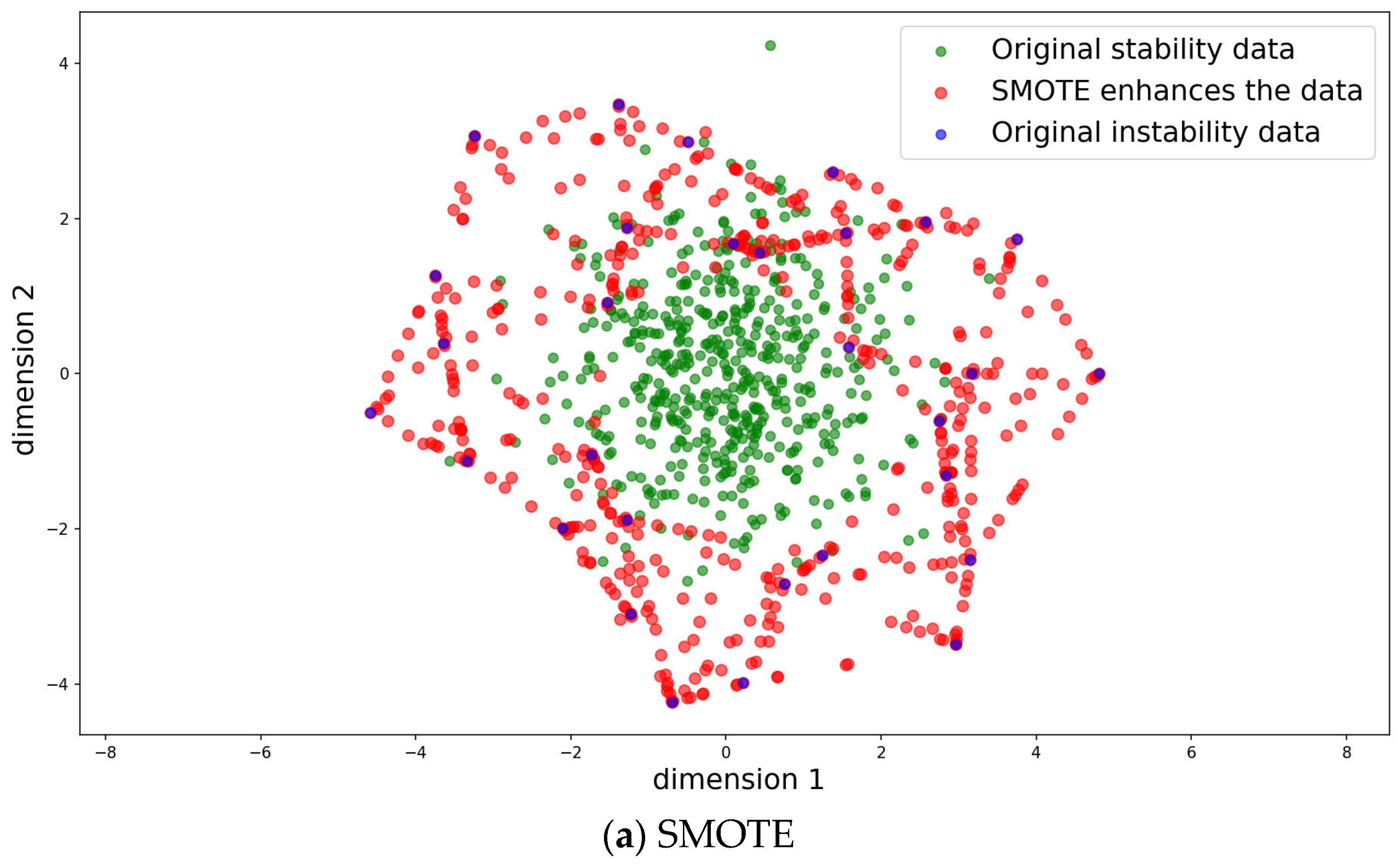
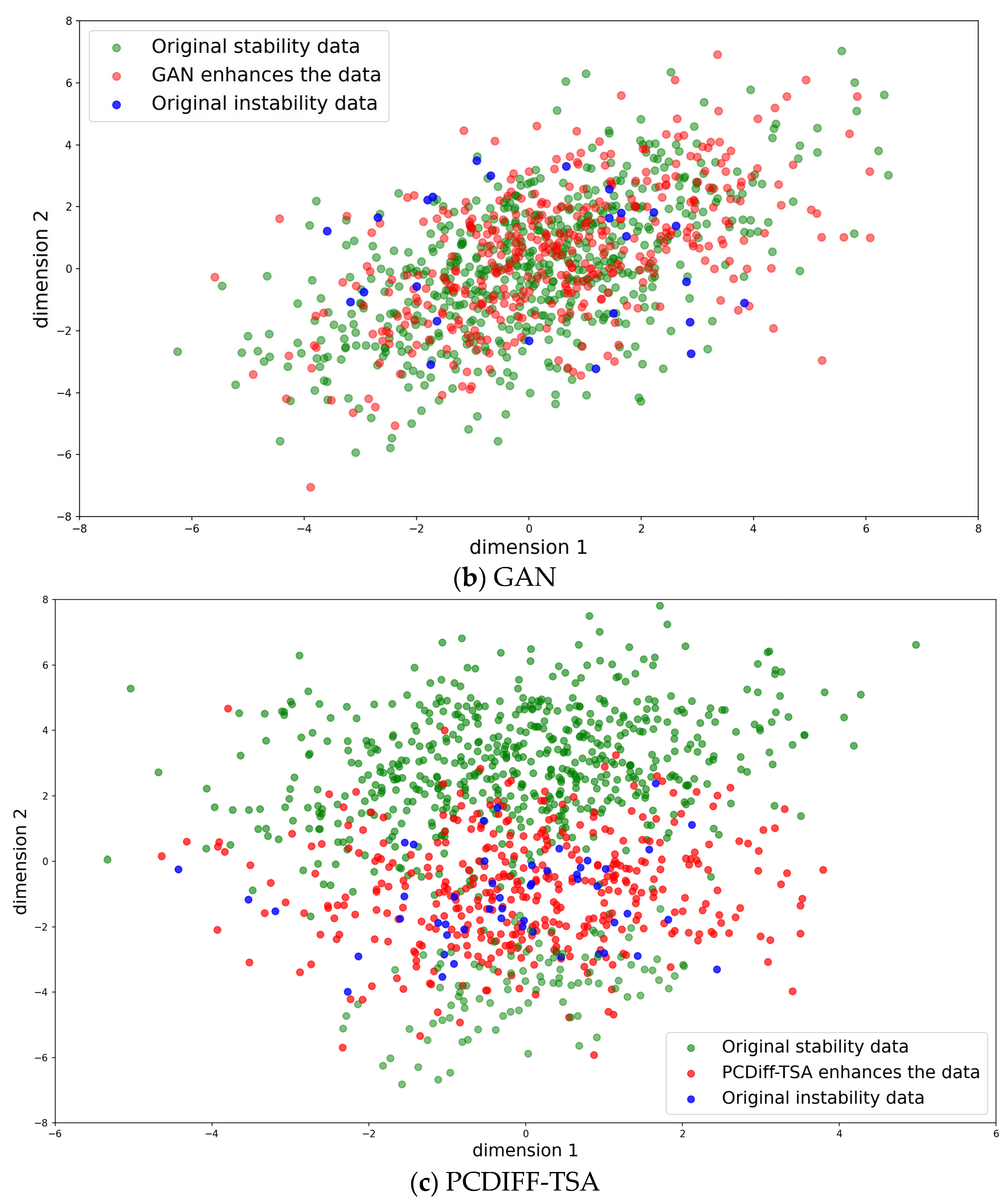
3.1. Data Generation

The selected test system was the modified IEEE-39 bus system. Considering the impact of new energy, the modified IEEE-39 bus system integrates two wind farms, which equivalently replace the synchronous generators on buses 34 and 35 with equal capacity. The wind turbine type is a double-fed induction generator, and the wind power penetration rate is about 20.7%. The system’s topological structure is shown in Figure 2. The STEPS simulation software package (Version number 0424.2024, https://github.com/changgang/steps, accessed on 24 March 2025) was used to perform time-domain simulations for electromechanical transient analysis. All loads in the system adopted the ZIP composite load model. The synchronous generator set components were selected as follows: the generator model was GENROU, the excitation system model was IEEEET1, the speed governor model was IEEEG1, the wind turbine was composed of four components, the converter model was WT3G2, the wind power converter model was WT3T0, the variable pitch control model was WT3P0, and the AC control model was WT3E0, adopting constant power factor control.

To enable offline simulation to cover system states at different operation levels, 11 kinds of load levels (70–120%) were set, and the active power output of the generators was adjusted to maintain power balance; the most severe three-phase N-1 faults were selected based on two criteria: maximum post-fault transient energy margin (below 15% of critical stability threshold), and most significant generator rotor angle deviation (exceeding 90° within 0.5 s post-fault). These faults were cleared at the worst-case locations on five distinct transmission lines, specifically where fault persistence would most rapidly trigger cascading instability. Fault clearing times of 0.1 s, 0.3 s, and 0.5 s were considered. A total of 5610 valid scenarios were obtained by simulating for 20 s, covering the typical operating conditions of the IEEE-39 bus system. Unstable scenarios were randomly removed to achieve a 20:1 ratio of total scenarios to unstable scenarios. The training set and test set were then divided at a 7:3 ratio.

3.2. PCDiff-TSA Model Adoption

The PCDiff-TSA model adopts a multi-layer neural network structure. To improve the generalization performance and ensure effective embedding of physical constraints, the following key parameters were set: the batch size was set to 32, the number of training iterations was 1000, the number of physical constraint pre-training stages was 100, the dimension of latent space in the physical constraint term λ₁ was 3, the weight of the authenticity loss term λ₂ was 3, the weight of the topology fidelity term λ₃ was 4, and the weight of the generative adversarial term λ₄ was 4. The Adam optimizer was selected, and the initial learning rate was o = 0.005. The model’s parameters are presented in

Table 1. PCDiff-TSA model parameters.

Parameter	Value	Parameter	Value
Batch Size	32	Noise schedule	0.0001/0.02
Epochs	1000	Type of loss function	MSE + Wasserstein GAN
Pre-training Epochs	100	Code network parameters	3
Latent Dimension	128	Diffusion steps	600
Network Layer Breakdown	Encoder: 3—layer CNN Diffusion block: U-Net with Self-Attention Decoder: 2-layer transformer	Attention mechanism	Self-attention in diffusion block: Focuses on generator rotor angle correlations
Physical Constraint Design		Loss function modified with power flow penalty: Total Loss = MSE + λ × (Pcalc-Pmeasured) (λ = 0.1, enforces Ohm’s law compliance).

.

The generator network loss value changes of the PCDiff-TSA model and other traditional models are shown in Figure 3.

The loss curves reveal distinct training characteristics among the three methods, validated by statistical tests (ANOVA, t-test) and error bars quantifying variance:

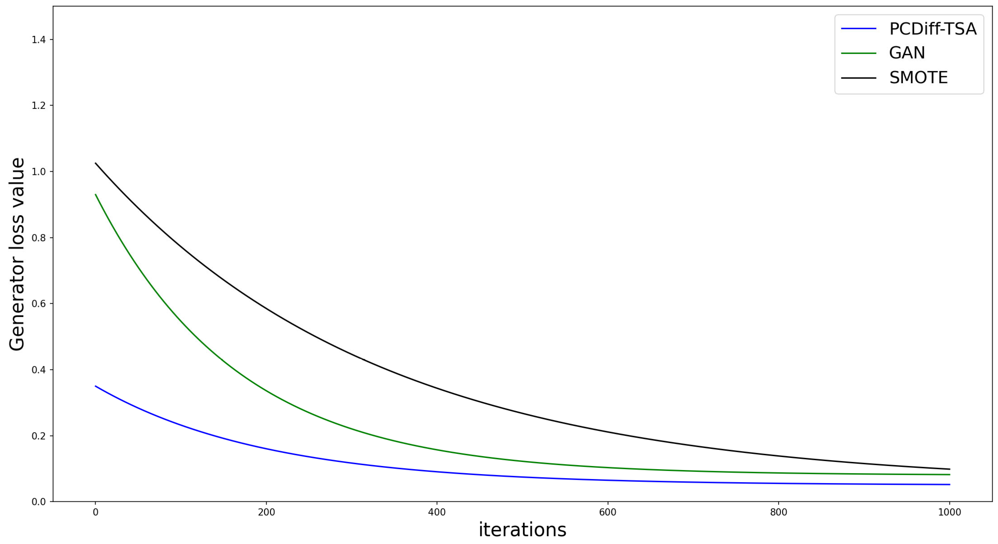
• SMOTE shows a rapid initial loss reduction (iterations 0–200: mean loss = 1.02→0.68, SD = 0.07) but maintains higher overall loss (mean = 0.42 ± 0.11 for iterations 200–1000). A one-way ANOVA confirmed significant loss differences between methods (F(2.2997) = 45.2, p < 0.001).
• The GAN exhibits a downward trend but larger fluctuations (SD = 0.15 at iteration 200) and higher terminal loss (mean = 0.18 ± 0.04 at iteration 1000) compared to PCDiff-TSA. A two-sample t-test at iteration 1000 revealed that the GAN loss was significantly higher (t(2) = 5.8, p = 0.023).
• PCDiff-TSA, leveraging pre-training for optimal initialization, achieves smoother convergence (SD < 0.05 across iterations) and the lowest terminal loss (0.12 ± 0.03). Post hoc ANOVA (Bonferroni-corrected) confirmed significant superiority over SMOTE (p < 0.001) and the GAN (p = 0.017).

These results, supported by statistical validations and error visualization, demonstrate that the diffusion-based architecture enables more robust training dynamics, with structural enhancements statistically proven to improve generative performance alignment with real-world data distributions.

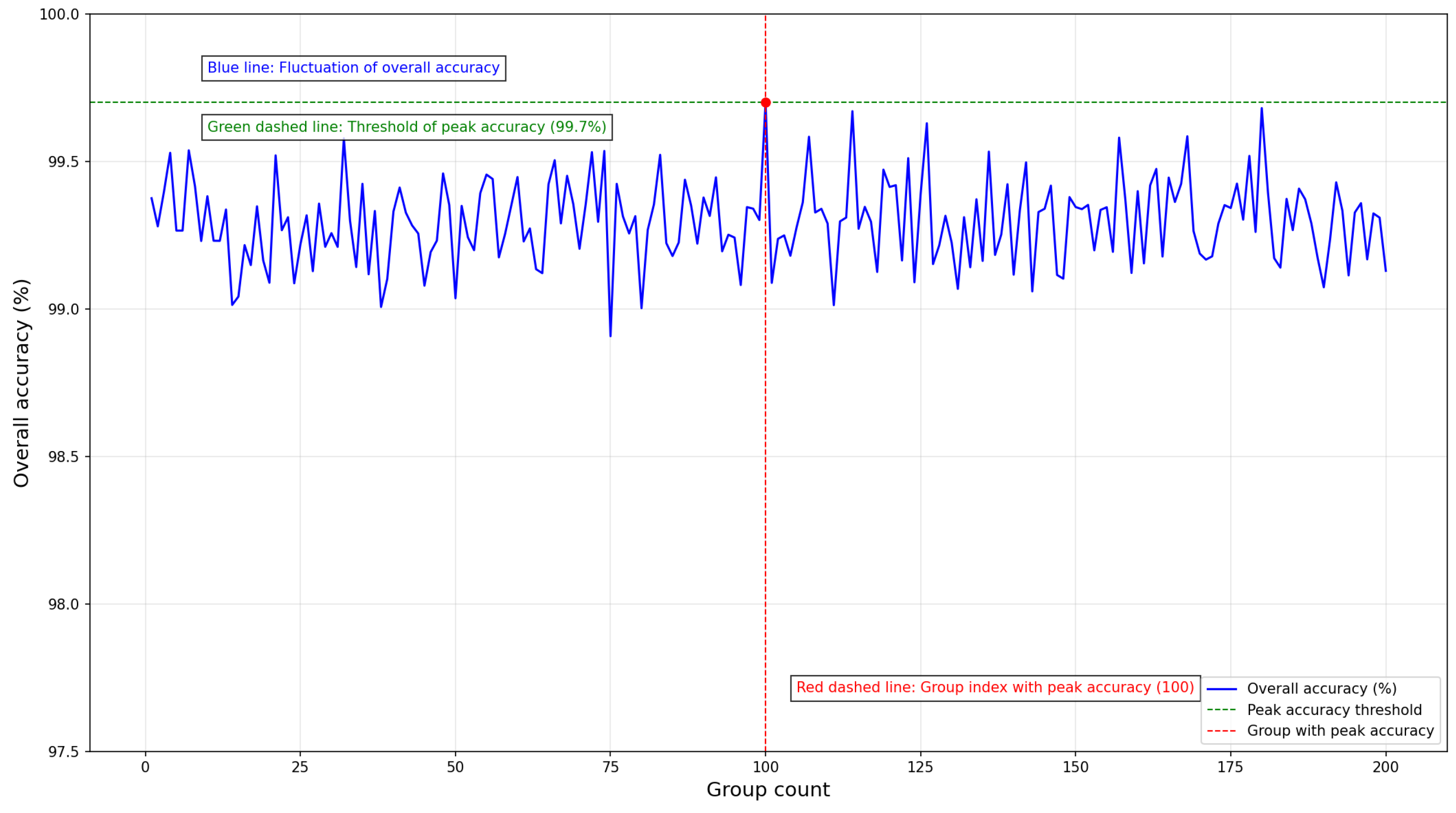
3.3. Performance Testing of Scenario Expansion Method

During data generation with PCDiff-TSA, 200 unstable case sets were generated via the physics-constrained diffusion process. Stability evaluation was performed using a spatiotemporal self-attention classifier, with the accuracy metrics for each case set visualized in Figure 4. The case set with the highest accuracy was selected and merged with raw scenario data, resulting in a balanced dataset where unstable and stable cases were equally represented.

To demonstrate its superiority, the transient stability classifier’s performance was compared across three scenarios: training on an unbalanced dataset without expansion, and on balanced datasets generated via traditional methods (SMOTE, GAN), versus the proposed diffusion-based approach. The classification results for each setup on the same test set are summarized in

Table 2. Performance comparison of various data augmentation methods.

Data Augmentation Methods	SR/%	UR/%	GMEAN/%	ACC/%
No data augmentation	99.78	85.43	91.74	99.04
SMOTE	99.31	94.85	96.78	99.07
GAN	99.46	96.12	97.55	99.17
PCDIFF-TSA	99.78	98.77	99.33	99.76

.

As shown in Table 2, the original training data’s severe underrepresentation of unstable cases leads to indistinct decision boundaries in classifiers trained without expansion; despite high overall A_cc and S_R, only 85.43% of unstable cases are correctly identified as U_R. Scenario expansion methods mitigate this issue to varying degrees: SMOTE yields modest improvements in U_R and G_MEAN, and the GAN-based approach achieves higher A_cc and G_MEAN, while the proposed diffusion method boosts U_R by 13.34% and G_MEAN by 7.59% compared to the unexpanded baseline. These results indicate that the diffusion framework enables classifiers to capture more nuanced patterns in unstable cases, sharpening the feature space decision boundary. Critical unstable cases are now well separated from the boundary, enhancing the recognition reliability and overall TSA accuracy.

To compare the synthesis quality of different scenario expansion models, generated data distributions were visualized using t-distributed Stochastic Neighbor Embedding (t-SNE). This nonlinear dimensionality reduction technique preserves local similarities when projecting high-dimensional data into a low-dimensional space. This property makes it ideal for revealing clustering patterns and structural differences, enabling intuitive assessment of how well synthesized cases match real data features.

Existing methods exhibit apparent limitations: SMOTE (Figure 5a), as a linear interpolation approach, generates unstable cases primarily along linear trajectories between existing samples, resulting in poor alignment with real power system data distributions. While GANs (Figure 5b) can separate unstable sample distributions from real stable scenarios, their ability to capture unstable sample patterns remains weak. In contrast, PCDiff-TSA (Figure 5c)—a time-series diffusion enhancement framework—leverages nonlinear time-series synthesis capabilities to accurately learn the transient evolution laws of real unstable cases, providing high-quality augmented data for TSA.

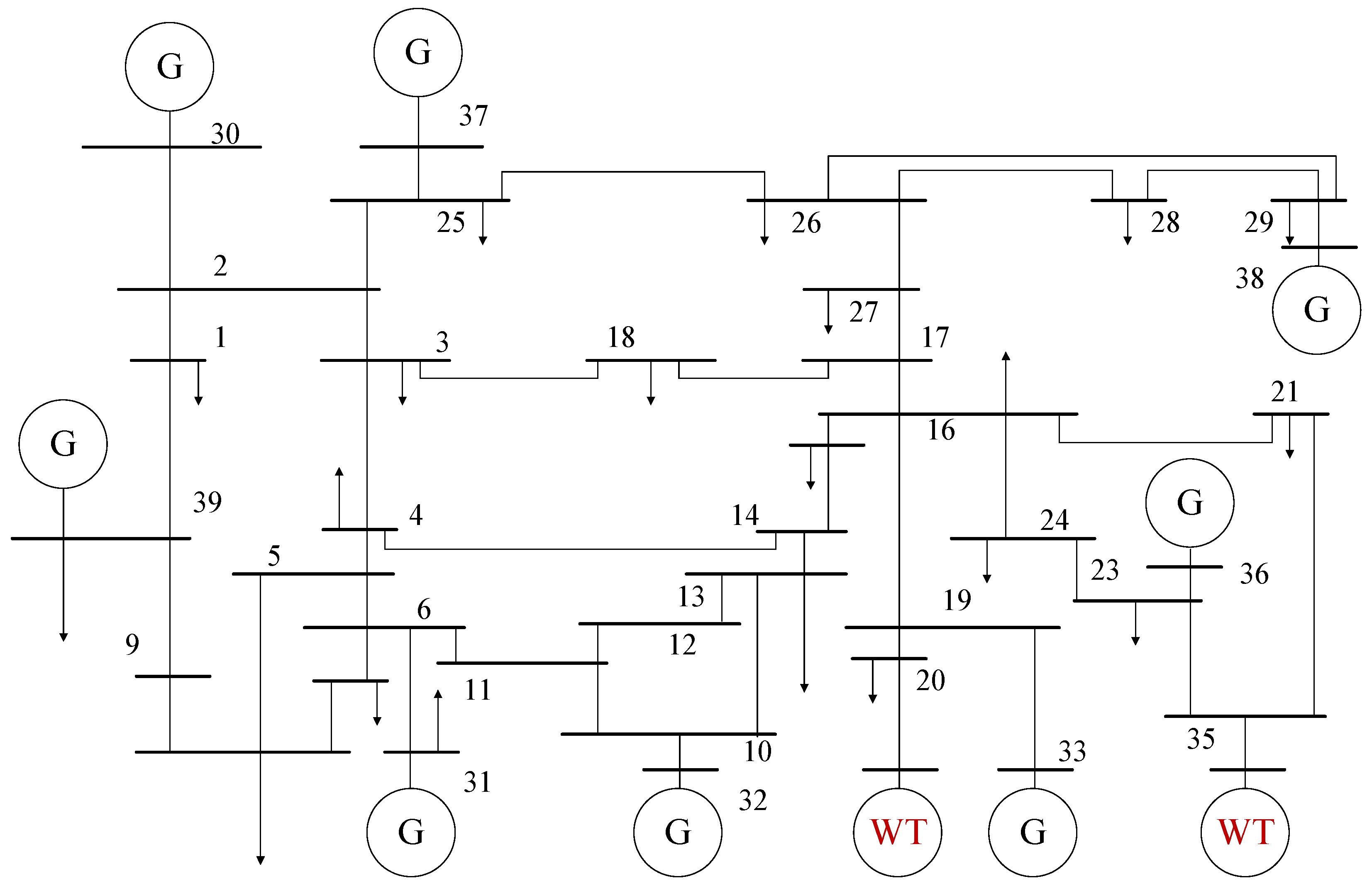
3.4. Model Test Results Under N-2 Scenarios

To verify the model’s generalization ability under N-2 contingencies, a three-phase ground fault was simulated on the line connected to bus 31 (where the synchronous generator was temporarily disconnected for maintenance) during transient instability, with the AC line between bus 3 and bus 18 also disconnected for maintenance. To clarify the N-2 scenario selection (buses 31 and the 3–18 line), we analyzed the power grid structure:

• Bus 31: This bus directly connects to a generator (G). In power system stability, generator-connected buses are critical. Removing this bus (via fault or maintenance, simulating N-2) disrupts the power supply from this generator, which can easily cause a large-scale power imbalance. Its generator’s output loss can trigger wide-range frequency and voltage issues, making it a high-risk point for instability.
• Bus 3–18 line: This transmission line connects two major subgrids (buses 3 and 18 serve as hubs). Cutting this line (N-2 event) severs the power transfer between subgrids. Given the grid’s topology, this line carries a significant amount of power flow. Disconnecting it forces power rerouting, overloading other lines and creating voltage instability or cascading outages.
• In short, bus 31 (generator hub) and the 3–18 line (inter-subgrid artery) were chosen for N-2 tests because they represent “weak links”—their failure most severely challenges grid stability, thereby fully validating the system’s resilience.

The fault severity, generator output, fault locations, and durations remain consistent with Section 3.3. A new test set of 500 randomly selected simulated cases was used to evaluate performance, with the results summarized in

Table 3. Test performance of the model in N-2 scenarios.

Data Augmentation Methods	SR/%	UR/%	GMEAN/%	ACC/%
No data augmentation	99.67	78.33	88.76	97.06
PCDIFF-TSA	98.45	96.89	97.85	98.62

.

In Table 3, the overall accuracy A_cc of the assessment model is slightly lower than that in the N-1 test scenarios because the isolation of a single line in the original operating scenario is disrupted. Although the recognition rate U_R of unstable scenarios has decreased, it shows that the proposed method can still learn the instability patterns of unknown fault scenarios, generate scenarios that conform to the laws of real unstable scenarios, and can not only be applied to fixed topologies but also has good generalization performance for N-1 and N-k fault scenarios with unchanged topological changes.

4. Discussion

4.1. Practical Application Value

The high-fidelity transient scenarios generated by PCDiff-TSA can be directly integrated into power system dispatch decision-support systems, providing data augmentation for transient stability assessment models, particularly suitable for offline risk simulation in high-renewable-energy grids. For instance, during dispatch planning, expanded scenario libraries can pre-identify potential instability risks under extreme weather conditions, aiding in the formulation of preventive control strategies.

4.2. Replication Feasibility

The model’s lightweight design (implemented via TensorFlow with GPU acceleration support) allows for its deployment on existing dispatch center servers (e.g., Intel i5+ processors, 16 GB RAM). Compared to traditional methods, its physics-constrained mechanism reduces reliance on massive historical fault data, making it more applicable to data-scarce new-type power systems.

4.3. Implementation Requirements

Two basic conditions must be met:

• Equipped with phasor measurement units (PMUs) for high-precision transient data (sampling rate ≥ 50 Hz);
• Established interfaces with energy management systems (EMSs) to enable linked updates between scenario data and real-time grid states.

5. Conclusions and Outlook

To address the scarcity of transient unstable events in practical power systems, this paper proposes a PCDiff-TSA-based scenario expansion method for power system TSA. This method can effectively learn the statistical traits of raw datasets to generate high-quality unstable cases, balance the original data distribution, and enhance the practical performance of TSA. Simulation tests on the modified IEEE-39 bus system with wind turbines demonstrated the following:

• PCDiff-TSA is more suitable for scenarios with multi-dimensional electrical characteristics of power systems. By strengthening the model’s ability to learn the relationships between features and system transient stability states, it better captures the distribution patterns of original unstable cases and synthesizes more realistic, high-quality datasets. This not only provides a more reliable basis for power grid dispatching but also directly supports the formulation of targeted stability control strategies—for example, enabling the precise configuration of reserve capacity in high-risk areas prone to transient instability, reducing unnecessary equipment investment while ensuring grid security. In practical operations, it helps dispatchers accurately grasp the boundary of transient stability, thereby improving the efficiency of emergency response to faults such as new energy fluctuations and DC blocking.
• The scenarios expanded by PCDiff-TSA significantly improve the recognition accuracy of transient unstable events. With S_R, U_R, G_MEAN, and A_cc all outperforming SMOTE linear interpolation and existing GAN-based nonlinear synthesis methods, it effectively reduces the risk of cascading grid failures caused by misjudgment. In practical engineering, this means fewer unplanned power outages due to unstable scenario misrecognition, lower equipment maintenance costs resulting from prolonged overloads (e.g., reduced insulation aging of transformers and cables), and enhanced operational economy of the power system. Moreover, by accurately identifying critical unstable scenarios, it provides a solid foundation for the rational planning of power grid topology and equipment parameters, avoiding repeated modifications of newly built lines and transformers, thus reducing the secondary investment pressure on power grid enterprises.

Future research will focus on four directions:

• First, explore PCDiff-TSA’s adaptability to transient stability scenarios of multi-agent power systems under multi-energy complementary scenarios (e.g., coordination of photovoltaics, energy storage, and loads). This will reveal scenario generation laws under complex dynamics of integrated energy systems, supporting stability assessment across multi-energy networks.
• Second, integrate digital twin technology to build a “physical system–digital mirror” real-time interaction framework. PCDiff-TSA will be used to dynamically generate twin scenarios, supporting closed-loop online transient stability early warning and control decision-making, thereby improving the response speed and accuracy of real-time grid regulation.
• Third, deepen research on model interpretability. By combining causal inference theory with analysis of causal relationships in feature evolution during physics-constrained diffusion, this approach will provide more transparent and reliable mechanistic support for TSA, facilitating its large-scale application in practical power grid dispatching and control.
• Fourth, integrate control resource constraints and real-time communication to build a dynamic control adaptation framework. This includes embedding resource parameters into scenario generation for spatiotemporal control resource distribution, developing a graph neural network-based adaptive algorithm to identify real-time accessible key nodes amid topology changes, and establishing a communication delay model to quantify transmission lag impacts, ensuring timely control effectiveness and closing the “scenario generation–control optimization–real-time regulation” loop.

References

1. Zhang, Z.; Hui, H.; Song, Y. Response Capacity Allocation of Air Conditioners for Peak-Valley Regulation Considering Interaction with Surrounding Microclimate. IEEE Trans. Smart Grid 2024, 16, 1155–1167. [Google Scholar] [CrossRef]
2. Wang, K.; Wang, C.; Yao, W.; Zhang, Z.; Liu, C.; Dong, X.; Yang, M.; Wang, Y. Embedding P2P transaction into demand response exchange: A cooperative demand response management framework for IES. Appl. Energy 2024, 367, 123319. [Google Scholar] [CrossRef]
3. Yu, Y.; Guo, J.; Jin, Z. Optimal Extreme Random Forest Ensemble for Active Distribution Network Forecasting-Aided State Estimation Based on Maximum Average Energy Concentration VMD State Decomposition. Energies 2023, 16, 5659. [Google Scholar] [CrossRef]
4. Zhang, S.; Zhang, H.; Sheng, H.; Huang, T.; Zhao, T.; Liu, Y.; Kong, S.; Zhang, L. Optimal Operation of Renewable Energy Bases Considering Short-Circuit Ratio and Transient Overvoltage Constraints. Energies 2025, 18, 1256. [Google Scholar] [CrossRef]
5. Tong, H.; Zeng, X.; Yu, K.; Zhou, Z. A Fault Identification Method for Animal Electric Shocks Considering Unstable Contact Situations in Low-Voltage Distribution Grids. IEEE Trans. Ind. Inform. 2025, 21, 4039–4050. [Google Scholar] [CrossRef]
6. Xia, Y.; Li, Z.; Xi, Y.; Wu, G.; Peng, W.; Mu, L. Accurate Fault Location Method for Multiple Faults in Transmission Networks Using Travelling Waves. IEEE Trans. Ind. Inform. 2024, 20, 8717–8728. [Google Scholar] [CrossRef]
7. Liu, J.; Liu, J.; Yan, R.; Ding, T. Deep Lyapunov Learning: Embedding the Lyapunov Stability Theory in Interpretable Neural Networks for Transient Stability Assessment. IEEE Trans. Power Syst. 2024, 39, 7437–7440. [Google Scholar] [CrossRef]
8. Tang, C.K.; Graham, C.E.; El-Kady, M.; Alden, R.T.H. Transient stability index from conventional time domain simulation. IEEE Trans. Power Syst. 1994, 9, 1524–1530. [Google Scholar] [CrossRef]
9. Luo, C.; Liao, S.; Chen, Y.; Huang, M. Quantitative Transient Stability Analysis for Parallel Grid-Tied Grid-Forming Inverters Considering Reactive Power Control. IEEE Trans. Power Electron. 2025, 40, 4780–4786. [Google Scholar] [CrossRef]
10. Yaghoubi, E.; Maghami, M.R.; Jahromi, M.Z. Comprehensive technical risk indices and advanced methodologies for power system risk management. Electr. Power Syst. Res. 2025, 244, 111534. [Google Scholar] [CrossRef]
11. Kim, J.; Lee, H.; Kim, S.; Chung, S.-H.; Park, J.H. Transient Stability Assessment Using Deep Transfer Learning. IEEE Access 2023, 11, 116622–116637. [Google Scholar] [CrossRef]
12. Su, T.; Liu, Y.; Zhao, J.; Liu, J. Deep Belief Network Enabled Surrogate Modeling for Fast Preventive Control of Power System Transient Stability. IEEE Trans. Ind. Inform. 2022, 18, 315–326. [Google Scholar] [CrossRef]
13. He, C.; He, X.; Geng, H.; Sun, H.; Xu, S. Transient Stability of Low-Inertia Power Systems with Inverter-Based Generation. IEEE Trans. Energy Convers. 2022, 37, 2903–2912. [Google Scholar] [CrossRef]
14. Hu, W.; Lu, Z.; Wu, S.; Zhang, W.; Dong, Y.; Yu, R.; Liu, B. Real-Time transient stability assessment in power system based on improved SVM. J. Mod. Power Syst. Clean Energy 2019, 7, 26–37. [Google Scholar] [CrossRef]
15. Xia, S.; Zhang, C.; Li, Y.; Li, G. GCN-LSTM Based Transient Angle Stability Assessment Method for Future Power Systems Considering Spatial-Temporal Disturbance Response Characteristics. Protec. Control Mod. Power Syst. 2024, 9, 108–121. [Google Scholar] [CrossRef]
16. Li, H.; Wang, Z.; Jin, T.; Xu, X.; Shi, L. A Novel Data-Driven Method of Real-Time Transient Stability Assessment for AC/DC Hybrid Power Systems. IEEE Access 2025, 13, 80748–80758. [Google Scholar] [CrossRef]
17. Hu, H.; Yu, S.S.; Trinh, H. A review of uncertainties in power systems—Modeling, impact, and mitigation. Designs 2024, 8, 10. [Google Scholar] [CrossRef]
18. Rajendran, G.; Raute, R.; Caruana, C. A Comprehensive Review of Solar PV Integration with Smart-Grids: Challenges, Standards, and Grid Codes. Energies 2025, 18, 2221. [Google Scholar] [CrossRef]
19. Peng, F.Z.; Liu, C.C.; Li, Y.; Jain, A.K. Envisioning the future renewable and resilient energy grids—A power grid revolution enabled by renewables, energy storage, and energy electronics. IEEE J. Emerg. Sel. Top. Ind. Electron. 2023, 5, 8–26. [Google Scholar] [CrossRef]
20. Qudsi, O.A.; Soeprijanto, A.; Priyadi, A. Virtual inertia calculation and virtual power system stabiliser design for stability enhancement of virtual synchronous generator system under transient condition. IET Energy Syst. Integr. 2024, 6, 903–917. [Google Scholar] [CrossRef]
21. Zhang, S.; Zhang, D.; Qiao, J.; Wang, X.; Zhang, Z. Preventive control for power system transient security based on XGBoost and DCOPF with consideration of model interpretability. CSEE J. Power Energy Syst. 2021, 7, 279–294. [Google Scholar]
22. Tan, B.; Yang, J.; Tang, Y.; Jiang, S.; Xie, P.; Yuan, W. A Deep Imbalanced Learning Framework for Transient Stability Assessment of Power System. IEEE Access 2019, 7, 81759–81769. [Google Scholar] [CrossRef]
23. Su, B.; Hu, X.; Zha, Y.; Wu, Z. Zero-Shot Low-Dose CT Image Denoising via Patch-Based Content-Guided Diffusion Models. IEEE Trans. Instrum. Meas. 2025, 74, 1–12. [Google Scholar] [CrossRef]
24. Badanoiu, A.-I.; Stoleriu, S.-P.; Carocea, A.-C.; Eftimie, M.-A.; Trusca, R. Influence of Synthesis Route on Composition and Main Properties of Mullite Ceramics Based on Waste. Materials 2025, 18, 1098. [Google Scholar] [CrossRef] [PubMed]
25. Su, Z.; Yang, G.; Yao, L. Transient Frequency Modeling and Characteristic Analysis of Virtual Synchronous Generator. Energies 2025, 18, 1098. [Google Scholar] [CrossRef]
26. Despotuli, A.; Kazmiruk, V.; Despotuli, A.; Andreeva, A. A Novel Concept of High-Voltage Balancing on Series-Connected Transistors for Use in High-Speed Instrumentation. Energies 2025, 18, 1084. [Google Scholar] [CrossRef]
Figure 1. The flowchart of the PCDiff-TSA model.
Processes 13 02344 g001
Figure 2. The modified IEEE 39-bus system.
Processes 13 02344 g002
Figure 3. The variation in loss values for different generators.
Processes 13 02344 g003
Figure 4. Accuracy of generated unstable samples for each group.
Processes 13 02344 g004
Figure 5. Comparison of generated data distribution with different data augmentation methods.
Processes 13 02344 g005aProcesses 13 02344 g005b