Automatic Delineation of Resistivity Contrasts in Magnetotelluric Models Using Machine Learning

Abstract

The precise identification of hydrocarbon-rich zones is crucial for optimizing exploration and production processes in the oil industry. Magnetotelluric (MT) surveys play a fundamental role in mapping subsurface geological structures. This study presents a novel methodology for automatically delineating resistivity contrasts in MT models by employing advanced machine learning and computer vision techniques. This approach commences with data augmentation to enhance the diversity and volume of resistivity data. Subsequently, a bilateral filter was applied to reduce noise while preserving edge details within the resistivity images. To further improve image contrast and highlight significant resistivity variations, contrast-limited adaptive histogram equalization (CLAHE) was employed. Finally, k-means clustering was utilized to segment the resistivity data into distinct groups based on resistivity values, enabling the identification of color features in different centroids. This facilitated the detection of regions with significant resistivity contrasts in the reservoir. From the clustered images, color masks were generated to visually differentiate the groups and calculate the area and proportion of each group within the pictures. Key features extracted from resistivity profiles were used to train unsupervised learning models capable of generalizing across different geological settings. The proposed methodology improves the accuracy of detecting zones with oil potential and offers scalable applicability to different datasets with minimal retraining, applicable to different subsurface environments. Ultimately, this study seeks to improve the efficiency of petroleum exploration by providing a high-precision automated framework with segmentation and contrast delineation for resistivity analysis, integrating advanced image processing and machine learning techniques. During initial analyses using only k-means, the resulting optimal value of the silhouette coefficient K was 2. After using bilateral filtering together with contrast-limited adaptive histogram equalization (CLAHE) and validation by an expert, the results were more representative, and six clusters were identified. Ultimately, this study seeks to improve the efficiency of petroleum exploration by providing a high-precision automated framework with segmentation and contrast delineation for resistivity analysis, integrating advanced image processing and machine learning techniques.

1. Introduction

Magnetotellurics (MT) has advanced significantly in recent decades and is a powerful geophysical tool for acquiring high-resolution information on lateral and vertical variations in electrical conductivity. These variations, which can be linked to geological resources and processes, are identified by simultaneously measuring natural fluctuations in electric and magnetic fields [1]. Such measurements cover a wide spectrum of frequencies, typically between 0.0001 Hz and 1000 Hz, enabling the study of the Earth’s structure from the upper kilometers of the crust to depths within the upper mantle [2,3,4]. A key advantage of this method is its noninvasive nature; as it does not require an active source to generate data, it offers substantial environmental benefits [2,5]. MT data interpretation involves converting electromagnetic signals from the time domain to the frequency domain. This conversion facilitates the determination of impedance values that are subsequently transformed into electrical resistivities at depth using inversion techniques [6].

Magnetotelluric resistivity profiles offer a detailed depiction of subsurface electrical properties [7,8], enabling the delineation of key geological features, such as the identification of subsurface fluids that can be linked to hydrocarbon reservoirs or magmatic and hydrothermal processes in the crust and mantle. Liu et al. [6]. reported that MT data may have limited resolution, especially at large depths, making it difficult to accurately distinguish boundaries between different geological units, particularly if the electrical properties of these units are similar [6]. While MT offers a technique that can provide answers to exploration questions in areas where interpretable seismic data is very difficult to acquire, it is difficult for MT to map buried resistive units within a highly conductive section [9]. The inherent limitations and uncertainties associated with magnetotelluric (MT) data require expert interpretation to reduce ambiguity. This study introduces an automated approach designed to augment this process, offering a robust method to assist and potentially standardize the delineation of subsurface boundaries.

MT interpretation faces several challenges reported in the literature, such as the nonuniqueness of the inversion problem, where multiple resistivity models can fit the data, making it difficult to obtain a unique solution [10,11,12]. Also, the geological heterogeneity generates a distortion of the electromagnetic signals and complicates the accuracy of the model [13,14]. To reduce these difficulties, different alternatives based on machine learning have been explored, including different machine learning algorithms, a sample-compressed neural network and an adaptive clustering analysis algorithm [6], representative massive resistivity models that employ advanced Deep Learning techniques adapted with Swin Transformer (SwinT) to improve inversion efficiency [15], DNN for producing accurate tomography inversion [16], convolutional neural networks (CNNs) for performing seismic impedance inversion [17], a deep residual CNN for one-dimensional audio magnetotelluric (AMT) inversion [18], and boundary demarcation including adaptive clustering analysis to segment regions in spatial data or images where the number of areas is not predefined by grouping the data into clusters based on distance to centroids [15]. But these approaches are particularly applied in the investment process. The application of computer vision techniques as a preprocessing stage, before the utilization of clustering algorithms on the geophysical models resulting from the inversion, is considerably advantageous. This approach can significantly improve the quality of the resulting segmentation and address inherent limitations in the direct application of algorithms like k-means to image data. K-means groups pixels based on feature similarities (e.g., intensity or color, which in this context represent resistivity values), but inherently lacks mechanisms to consider the spatial position or contiguity of these pixels.

In this context, we propose the development of an approach capable of processing large volumes of resistivity data using advanced computer vision algorithms, leveraging OpenCV in the RGB color space [16,17,18,19]. The goal was to create masks that can identify areas that exhibit significant resistivity contrasts. Using RGB images enables the extraction of rich, multidimensional information, thereby enhancing the classification accuracy of subsurface structures [20]. Previous studies have reported identification using image processing techniques, including fracture detection in satellite images [21,22,23], mineral identification from hyperspectral images [24,25], and soil classification in remote sensing studies [26,27]. Based on existing resistivity data, subsurface imaging from regions with hydrocarbon potential was automatically detected through machine learning models applied to resistivity profiles. These models are expected to generate semi-automatic frameworks with robust generalization capabilities across the resistivity ranges under investigation, allowing for the subsequent quantification of areas with contrasting resistivity that can be linked to the presence of hydrocarbons or other complex variations in rock properties, such as the presence of faults or rocks with different densities and fluids. The inherent limitations and uncertainties associated with the conventional processing of magnetotelluric (MT) data require expert interpretation to reduce ambiguity. Hence, to overcome this situation, this study introduces an automated approach designed to augment the data and the capacity of cluster identification, offering a robust method to assist and potentially standardize the delineation of subsurface boundaries. This research addressed the challenge of integrating advanced computer vision preprocessing (bilateral filtering, CLAHE) with clustering (k-means), specifically for MT resistivity model images, to improve contrast delineation without requiring large and labeled datasets. Additionally, there are no reported applications in the literature that integrate these methodologies and allow for standardizing the analysis process. This contrasts with some existing machine learning approaches, which can rely heavily on extensive image processing techniques before unsupervised clustering. This integrated sequence comprised several key stages: initial data augmentation; targeted image preprocessing, which employs bilateral filtering and contrast-limited adaptive histogram equalization (CLAHE) specifically adapted for MT resistivity images; and subsequent k-means. The overarching aim of this methodology is to effectively enhance subtle contrasts and automatically delineate features without reliance on pretrained models or extensive labeled datasets, thereby offering a potentially more flexible and efficient workflow for initial geophysical exploration.

2. Methods

This paper proposes a systematic methodology for the automatic delineation of resistivity contrasts in magnetotelluric models. By employing computer vision techniques, we aimed to improve the generalization capacity of classification models, facilitating the identification of areas with hydrocarbon production potential. The steps undertaken during the implementation are detailed below, and a general summary is presented in Figure 1.

2.1. Collection and Preparation of Resistivity Data

Magnetotelluric images from the subsurface were obtained from a magnetotelluric (MT) survey conducted in the Colombian Central Foothills, specifically in the Casanare and Boyacá regions. The field campaign utilized a linear array of 44 broadband induction coil MT stations distributed throughout 15 km, with an inter-station spacing of approximately 3.5 km. A remote reference station was located 38 km away in a low-noise area to improve data quality, and 16 vertical electrical soundings (VESs) were conducted. At each MT station, the north–south and east–west components of the electric and magnetic fields, along with the vertical magnetic field component, were independently measured, with a recording duration of approximately 20 h per station.

Data were collected using a Metronix ADU-07e system equipped with MFS-06e or MFS-07e coils, covering a frequency range of 0.1 to 1000 Hz. The initial sampling was conducted at 1024 Hz for the first 30 min, followed by a sampling rate of 128 Hz for the remaining acquisition period. Data processing was performed using the MAPROS software Ver. 0.87b, incorporating the Bounded Influence Remote Referencing (BIRRP) method [28]. This robust technique leverages remote referencing (RR) to reduce noise by ensuring synchronized acquisition between the remote station and each survey site, thereby enhancing the reliability of the impedance data through statistically robust processing techniques at selected frequencies. Galvanic distortion, commonly observed in MT data owing to near-surface conductivity heterogeneities [29], was mitigated using MAPROS, which applies spectral correlation and robust processing to eliminate incoherent noise. The final data inversion was conducted using WinGLink V.2.21, where 1D and 2D resistivity and phase models were generated. This process included editing the curves to remove outliers and applying joint inversion techniques, which corrected the inherent galvanic distortion, thereby refining the subsurface resistivity models.

2.2. Data Augmentation

Unsupervised data augmentation implies that the augmentation methods are not related to the data labels; they simply employ techniques that facilitate the generation of images that are later resized to ensure comparison in the classifiers [30]. For image classification tasks, image transformation methods without categories were used to generate new samples from the training set [31]. The image transformation methods used in this study are cropping, rotation, and flipping. The augmentation primarily served to test the algorithm’s invariance to these transformations and increase data points for evaluating the clustering consistency, resizing images post transformation to maintain consistent dimensions for analysis. However, specific geological complexities were not the aim of this augmentation strategy.

2.3. Image Preprocessing and Image Conversion and Restructuring

Image preprocessing, conversion, and restructuring are critical steps that prepare post-resistivity inversion data for effective analysis using machine learning and computer vision techniques [32]. These steps improve data quality, reduce noise, and format the data in a manner suitable for clustering algorithms such as k-means. A detailed description and mathematical demonstration of these processes follows:

Bilateral Filtering is an edge-preserving filter that can smoothen images and reduce noise. The pixel value of an output image is the weighted average of nearby pixels in the input image [33].

The bilateral filter can be formulated as follows:

$${\mathrm{BF}\left[\mathrm{I}\right]}_{\mathrm{p}}={\displaystyle \frac{1}{{\mathrm{W}}_{\mathrm{p}}}}{\displaystyle \sum }_{\mathrm{q}\mathrm{\in }\mathrm{S}}{\mathrm{G}}_{\mathrm{s}}\left(\Vert \mathrm{p}\text{-}\mathrm{q}\Vert \right){\mathrm{G}}_{\mathrm{r}}\left(\Vert {\mathrm{I}}_{\mathrm{p}}{\text{-}\mathrm{I}}_{\mathrm{q}}\Vert \right){\mathrm{I}}_{\mathrm{q}}$$

where

-

p and q are pixel locations in the image.

-

S is the neighborhood of pixel p.

-

G_s (ǁp-qǁ) is the spatial Gaussian kernel that decreases the influence of distant pixels in the spatial domain.

-

G_r (ǁI_p-I_qǁ) is the range Gaussian kernel, which decreases the influence of pixels with different intensities (resistivity values).

-

W_p is the normalization factor.

Contrast-limited adaptive histogram equalization (CLAHE) enhances the contrast of images by performing histogram equalization in small regions (tiles) of the image. This limits the amplification of noise by clipping the histogram to a predefined value (the contrast limit) [34]. The probability function P_x(i) considers any grayscale image (x), with n_i as the number of pixels with intensity level i, n as the total number of pixels, and L as the number of intensity levels in the image (x).

$${\mathrm{p}}_{\mathrm{x}}\left(\mathrm{i}\right)=\mathrm{p}\left(\mathrm{x}=\mathrm{i}\right)={\displaystyle \frac{{\mathrm{n}}_{\mathrm{i}}}{\mathrm{n}}}, 0 \le \mathrm{i} < \mathrm{L}$$

The above, with the respective conversions, allows the same analogy to be carried out in RGB channels.

2.4. Segmentation Using K-Means Clustering

There are different methods, and one of the most popular is the k-means clustering algorithm. The k-means clustering algorithm is unsupervised, and its main objective is to divide a dataset into a specific number of groups (clusters) where the objects within each group are as similar as possible; in the first phase, it calculates the k centroid, and in the second phase, each point is assigned to the cluster that has the nearest centroid from the respective data point [35]. There are different methods for defining the distance of the nearest centroid, and one of the most used methods is the Euclidean distance. K-means iteratively recalculates the centroids of each cluster and reassigns points to the cluster with the closest centroid based on Euclidean distance. K-means clustering was chosen due to its widespread use, computational efficiency, and effectiveness in partitioning data into a specified number of groups based on feature similarity (in this case, pixel color values in the processed images). Through this process, k-means minimizes the sum of the distances from each point to its centroid, thereby optimizing the cluster formation [36]. The k-means clustering algorithm is as follows [37]:

• Initialize the number of clusters k, and the center.
• For each pixel of an image, the Euclidean distance d between the center and each pixel of an image is calculated using the relationship given below:

$$\mathrm{d}=\Vert \mathrm{p}\left(\mathrm{x},\mathrm{y}\right){\text{-}\mathrm{c}}_{\mathrm{k}}\Vert$$

• Assign all the pixels to the nearest center based on distance d.
• After all the pixels have been assigned, the new position of the center is recalculated using the relationship given below:

$${\mathrm{c}}_{\mathrm{k}}={\displaystyle \frac{1}{\mathrm{k}}}{\displaystyle \sum }_{\mathrm{y}\mathrm{\in }{\mathrm{c}}_{\mathrm{k}}}{\displaystyle \sum }_{\mathrm{x}\mathrm{\in }{\mathrm{c}}_{\mathrm{k}}}\mathrm{p}(\mathrm{x},\mathrm{y})$$

This iterative process continues until convergence is reached, ensuring that the centroids stabilize and the segmentation accurately reflects the underlying patterns within the data. As a result, k-means effectively partitions the image into distinct regions, making it a powerful tool for feature extraction and classification in various applications.

3. Results

This section presents the results obtained in the analysis and identification of clusters in each processed image, highlighting the importance of using computer vision techniques that allow the processing of information, even with little data in this type of study. This section aims not only to describe the results but to offer an analysis of their accuracy and applicability in relation to the problem posed.

3.1. Cropping, Rotation, and Flipping

Image cropping, rotation, and flipping are effective data augmentation techniques that increase the dataset size. After applying these transformations, each image is resized based on field-collected information to maintain consistent dimensions and ensure a standardized format for analysis. These techniques enhance the model’s ability to recognize visual patterns across varying orientations and scales, thereby optimizing its performance in image classification and recognition tasks.

Figure 2 shows the division used in each image to identify the generalization capacity of the developed model. The dimensions for each cut were set at 4125 × 3333 pixels for later resizing to the real and representative spatial conditions of the information collection points in the field, as well as the scale of resistance recorded during the study.

Rotation, as a common method in data augmentation, allows rotation at a certain angle. In this case, 180° rotation was used, as shown in Figure 3a,b. This transformation allows for the observation of the application of the clusters and their concordance, regardless of the final orientation of the image. In many cases, after rotation, the dimensions of the image may change (particularly if the rotation angle is not a multiple of 90°) [38]. To avoid this and ensure that the model receives images of uniform size, the rotated images are resized to the original dimensions.

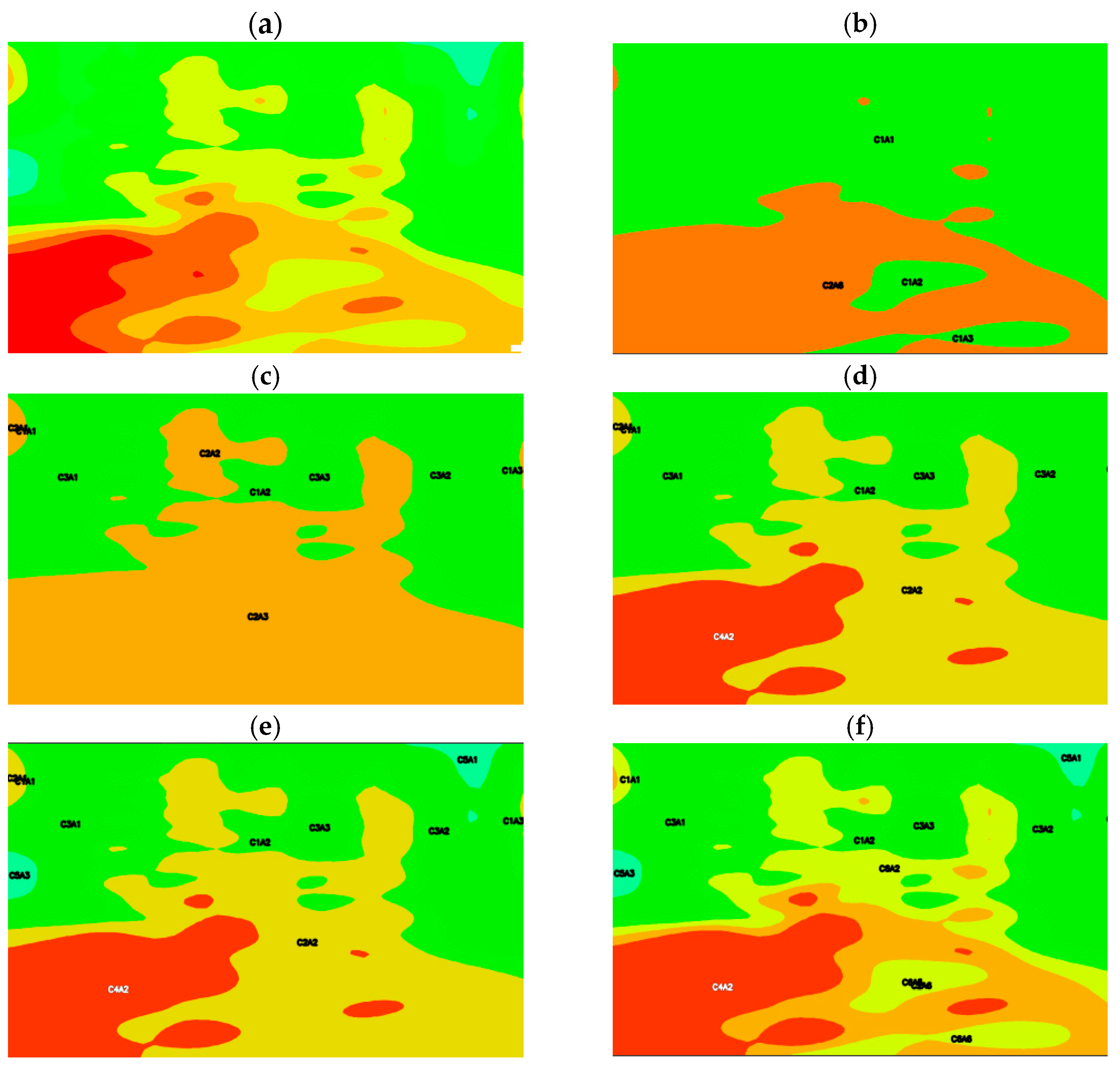
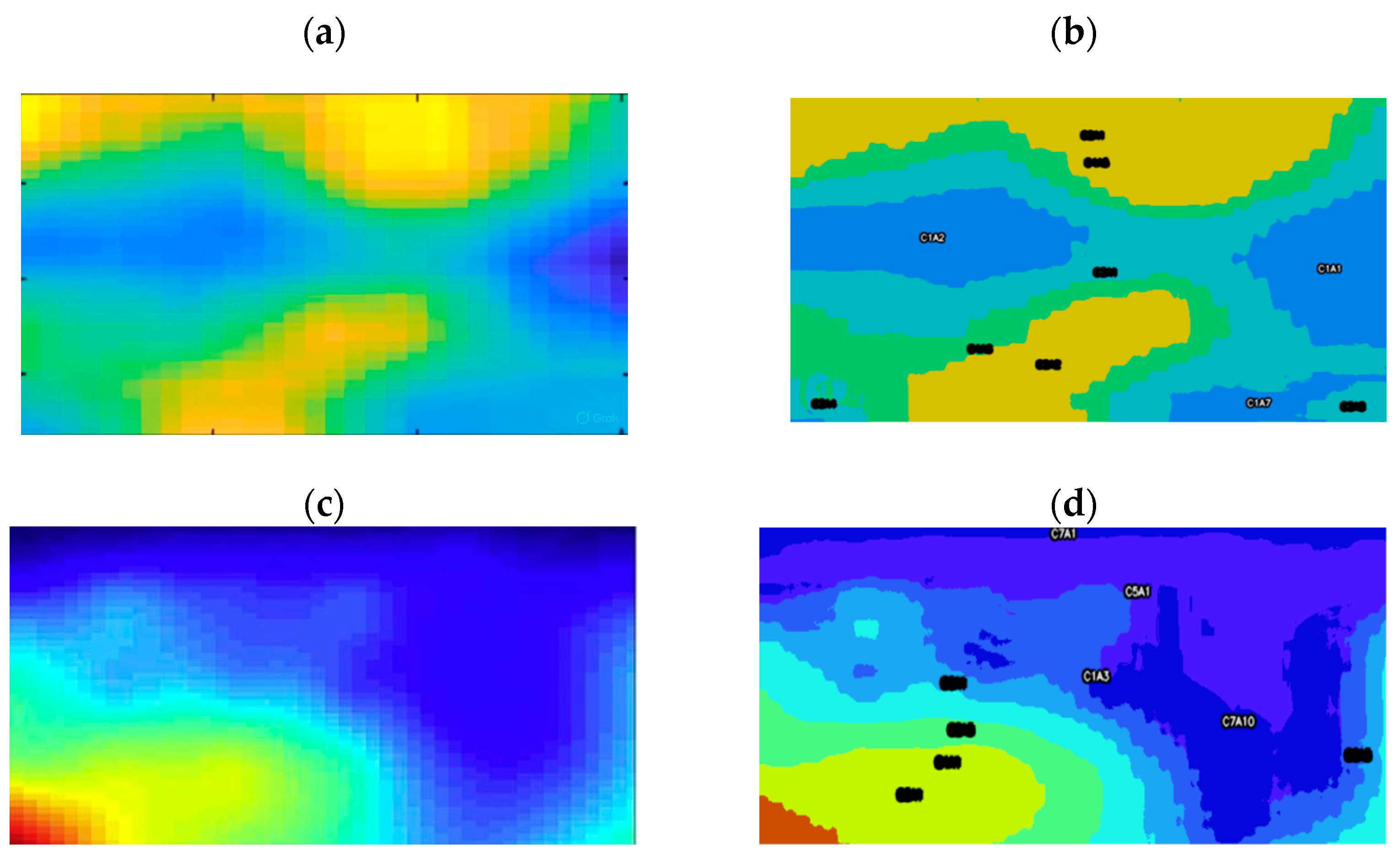
3.2. Classification by Resistivity Ranges Using K-Means

The use of k-means in conjunction with computer vision techniques is an alternative that has not yet been explored for this type of application. This anchoring allowed for the progressive identification of clusters, increasing the number of groups to highlight areas with a minimum of two clusters and a maximum of 10, using masks to identify the variation in the color channels in similar resistivity ranges in the images of interest.

A key advantage of this methodology is that it allows for the segmentation and grouping of pixels in different color ranges without the need for a large volume of training data or additional images, showing excellent results in the identification of areas for pictures without the need to train a dataset, considering the ability of computer vision techniques to identify groups of key features. This shows that by anchoring computer vision techniques to a clustering model such as k-means, it is possible to optimize the use of limited data volumes because segmentation and grouping reduce the dependence on large datasets. A key strength of this study is its ability to detect specific features within color channels that correlate with resistivity ranges observed in fieldwork, allowing for a more precise characterization of each area’s properties. However, one of the most important aspects to highlight is flexibility, scalability, and reduction in computational resources, as the application is facilitated to other images with identification characteristics that fit the maximum number of clusters defined (10). It is worth mentioning that the maximum number of clusters defined was 10 in this case, but the base code is adaptable to meet needs if expansion is required. The lower bound of K = 2 was chosen to explore segmentation at its broadest level, distinguishing major contrasting zones. The upper limit of K = 10 was established primarily to preserve the interpretative clarity of the results due to an excessive number of clusters tending to generate patterns that can be interpreted as noise. This was defined due to the frequency range of the equipment used to collect the data, which ranges from 0.1 Hz to 1000 Hz. This methodology is efficient in terms of processing and parallelization, indicating that it can be applied to multiple images without requiring intensive processing. Additionally,

Table 1. Cluster Distribution: Clusters, Pixel Count, Equivalent Area, and Total Percentage.

Cluster	Zone	Num. Pixels	Area (km2)	Percentage (%)
	C1A1	12,792	1364.19	0.83
	C1A2	225,623	24,061.40	14.58
	C1A3	13,412	1430.31	0.87
	C2A6	274,717	29,296.99	17.76
	C3A1	145,568	15,523.99	9.41
	C3A2	210,648	22,464.40	13.61
	C3A3	29,927	3191.54	1.93
	C4A2	238,898	25,477.10	15.44
	C5A1	16,483	1757.82	1.07
	C5A3	11,180	1192.28	0.72
	C6A2	250,254	26,688.15	16.17
	C6A5	39,458	4207.97	2.55
	C6A6	41,249	4398.97	2.67

provides a summary of each group identified in the image. To prevent excessive data saturation within the visualization, a filtering criterion was applied, retaining only regions that occupy more than 0.5% of the total image area. Therefore, the sum of these data was 97% of the total area (Figure 4).

Figure 5 shows a bar graph representing the proportion of pixels (or areas) corresponding to each cluster identified in the final resistivity analysis process. The vertical axis shows the proportion of pixels (relationship to the total pixels), and the horizontal axis shows different clusters. Cluster 3 had the highest proportion of pixels, with 24.95% of the total area, followed by Clusters 4, 6, and 5. In this case, Cluster 4 stands out, as it is the area that, depending on the type of rock, porosity, and the observed resistivity range, allows us to infer an area in the presence of hydrocarbons, taking into account the resistivity value identified in the study area. Cluster 1 had the lowest proportion of pixels (9.77%). This graph provides a clear visualization of how the total area is distributed among different clusters, which allows the regions of interest within the dataset to be automatically delimited. The established geological interpretation of the area allows for the detected resistivity ranges to be correlated with the groups described in

Table 2. Geological Interpretation of Delineated Resistivity Clusters.

Cluster	Zone	Geological Interpretation
	C1A1	Clay
	C1A2	Clay
	C1A3	Clay
	C2A6	Sandstone bearing oil
	C3A1	Shale
	C3A2	Shale
	C3A3	Shale
	C4A2	High-saturation hydrocarbon-bearing sandstone
	C5A1	Fresh Water
	C5A3	Fresh Water
	C6A2	Sandstone
	C6A5	Sandstone
	C6A6	Sandstone

for this zone.

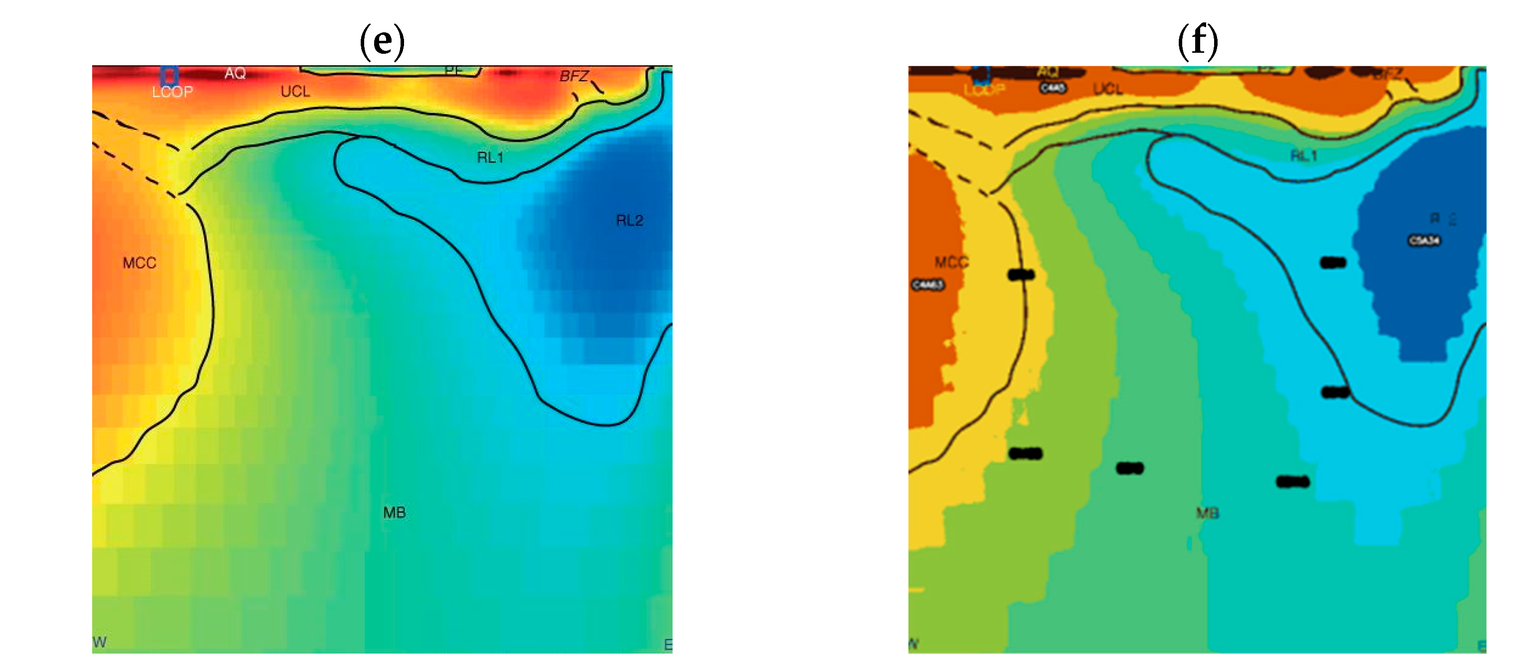
3.3. Model Validation and Generalization Capability

This section presents the validation results obtained by applying the developed model to previously published images. The aim of the adaptive clustering algorithm was not only to identify the number of clusters, but also to demarcate the boundaries of these clusters. In Article A. Liu et al. (2020) [6], Application of Sample-Compressed Neural Network and Adaptive-Clustering Algorithm for Magnetotelluric Inverse Modeling, the dimensions were 1000 m horizontally and 500 m vertically with a resistivity range of 0–280 [Ω m]. In Article B. Giuseppe et al. (2014) [15], K-Means Clustering as a Tool for Multivariate Geophysical Data Analysis, the dimensions were 290 m horizontally and 100 m vertically, with a resistivity range of 0–5000 [Ω m]. An application to shallow fault zone imaging, Article C. Beka et al. (2015) [39], The First Magnetotelluric image of the Lithospheric-Scale Geological Architecture in Aentral Svalbard, Arctic Norway, the dimensions were 27,000 m horizontally and 30,000 m vertically with a resistivity range of 0–4000 [Ω m]. These studies were selected due to their value for the understanding of the subsurface history and the relevance of their data for assessing the generalization capabilities of the proposed method. Figure 6a,c,e illustrate the original images from the referenced articles, while Figure 6b,d,f display the corresponding outputs processed by the model developed in this study.

The results demonstrate the developed model’s capacity to accurately identify and delineate resistivity contrasts described in the original studies. The approximate processing time for the complete workflow (preprocessing and clustering) on a representative MT image, utilizing standard computational resources, is 0.13 s. This processing efficiency underscores the method’s suitability for rapid analysis. Furthermore, this validation exercise underscores the robustness of the model in adapting to diverse geological scenarios and its ability to reproduce key observations reported in independent studies, thereby supporting its potential for broader applicability.

4. Conclusions

The integration of specific computer vision preprocessing techniques (bilateral filtering, CLAHE) with unsupervised clustering (k-means) adapted for MT resistivity profile images allows for the enhanced, automated delineation of resistivity contrasts, potentially using limited data and without complex model training, offering a practical workflow addition to existing MT interpretation tools. A rigorous data quality control process was implemented, encompassing the sensor calibration and data coherence verification. The proposed methodology enhances the precision of identifying potential hydrocarbon-bearing zones and provides a scalable solution applicable to diverse geological settings. This is achieved by integrating image processing and machine learning techniques, employing computer vision methods such as bilateral filtering for noise reduction, and contrast-limited adaptive histogram equalization (CLAHE) for image contrast enhancement. Subsequently, the processed images underwent pixel-based thresholding clustering using k-means to segment resistivity data into distinct groups based on resistivity values, facilitating the detection of regions with significant contrasts. The methodology demonstrated its ability to optimize the utilization of limited data, exhibiting promising results in identifying target areas without requiring extensive training data. The interpretability challenge common to unsupervised methods like k-means, that the resulting clusters are based on data patterns (color/resistivity values in the image) and do not guarantee direct correspondence to specific geological units without further interpretation.

References

1. Chave, A.D.; Jones, A.G. The Magnetotelluric Method: Theory and Practice; Cambridge University Press: Cambridge, UK, 2012. [Google Scholar]
2. Simpson, F.; Bahr, K. Practical Magnetotellurics; Cambridge University Press: Cambridge, UK, 2005. [Google Scholar]
3. Rycroft, M.J.; Harrison, R.G.; Nicoll, K.A.; Mareev, E.A. An overview of Earth’s global electric circuit and atmospheric conductivity. Planet. Atmos. Electr. 2008, 137, 83–105. [Google Scholar]
4. Everett, M.E. Near-Surface Applied Geophysics; Cambridge University Press: Cambridge, UK, 2013. [Google Scholar]
5. Spichak, V.V. Advances in electromagnetic techniques for exploration, prospecting, and monitoring of hydrocarbon deposits. First Break 2018, 36, 75–81. [Google Scholar] [CrossRef]
6. Liu, W.; Lü, Q.; Yang, L.; Lin, P.; Wang, Z. Application of sample-compressed neural network and adaptive-clustering algorithm for magnetotelluric inverse modeling. IEEE Geosci. Remote Sens. Lett. 2020, 18, 1540–1544. [Google Scholar] [CrossRef]
7. Lin, W.; Yang, B.; Han, B.; Hu, X. A review of subsurface electrical conductivity anomalies in magnetotelluric imaging. Sensors 2023, 23, 1803. [Google Scholar] [CrossRef] [PubMed]
8. Liu, X.; Craven, J.A.; Tschirhart, V. Retrieval of Subsurface Resistivity from Magnetotelluric Data Using a Deep-Learning-Based Inversion Technique. Minerals 2023, 13, 461. [Google Scholar] [CrossRef]
9. Christopherson, K.R. Applications of magnetotellurics to petroleum exploration in Papua New Guinea: A model for frontier areas. Lead. Edge 1991, 10, 21–27. [Google Scholar] [CrossRef]
10. Gallardo, L.A.; Meju, M.A. Joint two-dimensional cross-gradient imaging of magnetotelluric and seismic traveltime data for structural and lithological classification. Geophys. J. Int. 2007, 169, 1261–1272. [Google Scholar] [CrossRef]
11. Yin, C. Inherent nonuniqueness in magnetotelluric inversion for 1D anisotropic models. Geophysics 2003, 68, 138–146. [Google Scholar] [CrossRef]
12. Muñoz, G.; Rath, V. Beyond smooth inversion: The use of nullspace projection for the exploration of non-uniqueness in MT. Geophys. J. Int. 2006, 164, 301–311. [Google Scholar] [CrossRef]
13. Park, S.K. Mantle heterogeneity beneath eastern California from magnetotelluric measurements. J. Geophys. Res. Solid Earth 2004, 109, B9. [Google Scholar] [CrossRef]
14. Plotkin, V. Inversion of heterogeneous anisotropic magnetotelluric responses. Russ. Geol. Geophys. 2012, 53, 829–836. [Google Scholar] [CrossRef]
15. Di Giuseppe, M.G.; Troiano, A.; Troise, C.; De Natale, G. k-Means clustering as tool for multivariate geophysical data analysis. An application to shallow fault zone imaging. J. Appl. Geophys. 2014, 101, 108–115. [Google Scholar] [CrossRef]
16. Kumar, E.B.; Thiagarasu, V. Color channel extraction in RGB images for segmentation. In Proceedings of the 2nd International Conference on Communication and Electronics Systems (ICCES), Coimbatore, India, 19–20 October 2017; pp. 234–239. [Google Scholar]
17. Rajinikanth, V.; Couceiro, M. RGB histogram based color image segmentation using firefly algorithm. Procedia Comput. Sci. 2015, 46, 1449–1457. [Google Scholar] [CrossRef]
18. Kulkarni, N. Color thresholding method for image segmentation of natural images. Int. J. Image Graph. Signal Process. 2012, 4, 28. [Google Scholar] [CrossRef]
19. Henderson, J.; Purves, S.J.; Fisher, G.; Leppard, C. Delineation of geological elements from RGB color blending of seismic attribute volumes. Lead. Edge 2008, 27, 342–350. [Google Scholar] [CrossRef]
20. Savelonas, M.A.; Veinidis, C.N.; Bartsokas, T.K. Computer Vision and Pattern Recognition for the Analysis of 2D/3D Remote Sensing Data in Geoscience: A Survey. Remote Sens. 2022, 14, 6017. [Google Scholar] [CrossRef]
21. Zeeb, C.; Göckus, D.; Bons, P.; Al Ajmi, H.; Rausch, R.; Blum, P. Fracture flow modelling based on satellite images of the Wajid Sandstone, Saudi Arabia. Hydrogeol. J. 2010, 18, 1699. [Google Scholar] [CrossRef]
22. Rubanga, D.P.; May-Cuevas, S.A.; Arvelyna, Y.; Shimada, S. Fracture-fault detection using deep learning with stepwise elimination from satellite images in Djibouti. GEOMATE J. 2023, 25, 241–248. [Google Scholar]
23. Koike, K.; Nagano, S.; Kawaba, K. Construction and analysis of interpreted fracture planes through combination of satellite-image derived lineaments and digital elevation model data. Comput. Geosci. 1998, 24, 573–583. [Google Scholar] [CrossRef]
24. Okada, N.; Maekawa, Y.; Owada, N.; Haga, K.; Shibayama, A.; Kawamura, Y. Automated identification of mineral types and grain size using hyperspectral imaging and deep learning for mineral processing. Minerals 2020, 10, 809. [Google Scholar] [CrossRef]
25. Sudharsan, S.; Hemalatha, R.; Radha, S. A survey on hyperspectral imaging for mineral exploration using machine learning algorithms. In Proceedings of the 2019 International Conference on Wireless Communications Signal Processing and Networking (WiSPNET), Chennai, India, 21–23 March 2019; pp. 206–212. [Google Scholar]
26. Vibhute, A.D.; Kale, K.; Dhumal, R.K.; Mehrotra, S. Soil type classification and mapping using hyperspectral remote sensing data. In Proceedings of the 2015 International Conference on Man and Machine Interfacing (MAMI), Bhubaneswar, India, 17–19 December 2015; pp. 1–4. [Google Scholar]
27. Demanet, D.; Pirard, E.; Renardy, F.; Jongmans, D. Application and processing of geophysical images for mapping faults. Comput. Geosci. 2001, 27, 1031–1037. [Google Scholar] [CrossRef]
28. Chave, A.D.; Thomson, D.J. A bounded influence regression estimator based on the statistics of the hat matrix. J. R. Stat. Soc. Ser. C Appl. Stat. 2003, 52, 307–322. [Google Scholar] [CrossRef]
29. Bibby, H.; Caldwell, T.; Brown, C. Determinable and non-determinable parameters of galvanic distortion in magnetotellurics. Geophys. J. Int. 2005, 163, 915–930. [Google Scholar] [CrossRef]
30. Shijie, J.; Ping, W.; Peiyi, J.; Siping, H. Research on data augmentation for image classification based on convolution neural networks. In Proceedings of the 2017 Chinese Automation Congress (CAC), Tianjin, China, 20–22 October 2017; pp. 4165–4170. [Google Scholar]
31. Ioffe, S. Batch normalization: Accelerating deep network training by reducing internal covariate shift. arXiv 2015, arXiv:1502.03167. [Google Scholar]
32. Rama, J.; Nalini, C.; Kumaravel, A. Image pre-processing: Enhance the performance of medical image classification using various data augmentation technique. Accent. Trans. Image Process. Comput. Vis. 2019, 5, 7. [Google Scholar] [CrossRef]
33. Lin, T.H.; Way, D.L.; Shih, Z.C.; Tai, W.K.; Chang, C.C. An efficient structure-aware bilateral texture filtering for image smoothing. In Computer Graphics Forum; Wiley Online Library: Hoboken, NJ, USA, 2016; Volume 35, pp. 57–66. [Google Scholar]
34. Yadav, G.; Maheshwari, S.; Agarwal, A. Contrast limited adaptive histogram equalization based enhancement for real time video system. In Proceedings of the 2014 International Conference on Advances in Computing, Communications and Informatics (ICACCI), Bangalore, India, 19–20 September 2014; pp. 2392–2397. [Google Scholar]
35. Khan, S.S.; Ahmad, A. Cluster center initialization algorithm for K-means clustering. Pattern Recognit. Lett. 2004, 25, 1293–1302. [Google Scholar] [CrossRef]
36. Dhanachandra, N.; Manglem, K.; Chanu, Y.J. Image segmentation using K-means clustering algorithm and subtractive clustering algorithm. Procedia Comput. Sci. 2015, 54, 764–771. [Google Scholar] [CrossRef]
37. Salihah, A.-N.A.; Yusoff, M.; Zeehaida, M. Colour image segmentation approach for detection of malaria parasites using various colour models and k-means clustering. WSEAS Trans. Biol. Biomed. 2013, 10, 41–55. [Google Scholar]
38. Szeliski, R. Shape from Rotation; Citeseer: Cambridge, MA, USA, 1990. [Google Scholar]
39. Beka, T.I.; Smirnov, M.; Bergh, S.G.; Birkelund, Y. The first magnetotelluric image of the lithospheric-scale geological architecture in central Svalbard, Arctic. Norway Polar Res. 2015, 34, 26766. [Google Scholar] [CrossRef]
Figure 1. Flowchart of the Proposed Methodology.
Processes 13 02263 g001
Figure 2. Image division and associated resistivity distribution.
Processes 13 02263 g002
Figure 3. Rotation and data volume increase: (a) presents the original or reference image. (b) presents the original image rotated 180° and resized.
Processes 13 02263 g003
Figure 4. Summary of evaluated clusters to image A23. (a) original, (b) 2 clusters, (c) 3 clusters, (d) 4 clusters, (e) 5 clusters, and (f) 6 clusters.
Processes 13 02263 g004
Figure 5. Cluster Area Distribution in Resistivity Analysis.
Processes 13 02263 g005
Figure 6. Comparison between original images (a,c,e) and processed results (b,d,f). The original images are taken from [6,15,39], while the results show the automatic identification of resistivity contrasts using the proposed model.
Processes 13 02263 g006aProcesses 13 02263 g006b