1. Introduction
Since the proposal of the “dual-carbon” goal, China has actively advanced the development of renewable energy to address climate change and enhance energy security. Among these sources, wind power plays a crucial role due to its renewable nature, low cost, and zero emissions, leading to its growing presence in the national energy mix [
1]. Nevertheless, the inherent variability and unpredictability of wind power often result in generation intermittency, which complicates energy utilization and poses technical challenges for grid integration. Accurate forecasting of wind power can help overcome these issues by supporting effective grid scheduling and ensuring the stable operation of wind-connected systems [
2,
3].
Short-term wind power forecasting models are generally categorized into three types: physical models, statistical models, and hybrid (combined) models [
4]. Physical models [
5] rely on meteorological forecasts and turbine characteristics specific to geographic locations. Although useful for long-term predictions, their reliance on extensive and complex weather data limits their accuracy and practicality for short-term forecasting. Statistical models [
6], on the other hand, establish data-driven relationships between inputs—such as numerical weather forecasts and historical generation data—and predicted outputs. These models are simpler to construct and often yield better accuracy and generalization than physical models. However, their performance can vary across different time scales, especially when handling nonlinear patterns, potentially resulting in larger prediction errors. To overcome the limitations of both approaches, hybrid models integrate optimization algorithms with prediction techniques [
7], enabling more accurate modeling of wind speed and power fluctuations. By tuning model parameters through optimization, these combined approaches enhance forecasting accuracy and robustness, meaning that they are widely adopted in modern wind power prediction tasks.
At present, conventional single prediction models include the neural network prediction model [
8], the integrated learning [
9] prediction model and the Random Forest [
10] (RF) prediction model. Optimization algorithms mainly include Particle Swarm Optimization [
11] (PSO), Genetic Algorithm (GA) and Differential Evolution (DE).
An enhanced PSO-BP model was introduced [
12], where Particle Swarm Optimization (PSO) was used to optimize the weights and thresholds of the BP neural network. However, due to the BP network’s reliance on gradient descent, it is prone to getting trapped in local optima, indicating the need for more advanced neural network architectures to address this limitation. In [
13], a forecasting method utilizing the Spotted Hyena Algorithm (SHA) was proposed to optimize the penalty coefficients and kernel parameters of the Support Vector Machine (SVM), resulting in notable improvements in prediction accuracy and stability. Ref. [
14] presented a wind power prediction model combining the Sparrow Search Algorithm (SSA) with a Gated Recurrent Unit (GRU), where SSA is employed to fine-tune model parameters through iterative optimization, enhancing forecasting performance. These hybrid approaches illustrate the effectiveness of integrating optimization algorithms with predictive models to address the uncertainty and volatility inherent in wind power forecasting.
Given the stochastic, volatile, and long-tailed characteristics of wind power sequences, many current hybrid models incorporate signal decomposition techniques to simplify data structure and enhance forecasting accuracy. These methods help reduce the complexity and randomness of the original signal, making them widely adopted in wind power data preprocessing. Common techniques include Fourier Transform [
15] (Fast Fourier Transform, FFT), Empirical Mode Decomposition (EMD) [
16], and others. For instance, Ref. [
17] presents an EMD-based hybrid model that integrates an improved GA-BP algorithm with Adaboost, introducing a novel hidden layer node selection strategy. By applying EMD to obtain decomposed input data, the model improves prediction accuracy by capturing relationships between components and the output. However, EMD, despite its suitability for nonlinear and non-smooth signals, suffers from issues like mode mixing and sensitivity to boundary effects, limiting its robustness. In contrast, Variational Mode Decomposition (VMD) [
18] offers a more stable approach by breaking down highly volatile and random sequences into multiple smooth and regular subcomponents, effectively preserving the intrinsic power characteristics of the original data while enhancing consistency.
To address the challenge of improving both accuracy and stability in short-term wind power forecasting, this study proposes a hybrid prediction model that integrates the Northern Goshawk Optimization (NGO) algorithm and an Improved Snow Ablation Optimizer (ISAO) within a VMD-LSTM framework. First, Variational Mode Decomposition (VMD) is applied to break down the original wind power sequence into multiple components. The NGO algorithm is employed to optimize the key VMD parameters [k,α], using minimum alignment entropy as the fitness criterion, thus enhancing the decomposition’s effectiveness by reducing noise and ensuring more stable input for the forecasting stage. Next, a separate LSTM model is constructed for each decomposed component, with ISAO used to fine-tune the LSTM hyperparameters, resulting in the ISAO-LSTM forecasting model. After training with the optimized parameters, the final output is generated through the reconstruction of individual predictions. Experimental results confirm that the proposed approach significantly enhances forecasting accuracy and robustness.
3. Short-Term Wind Power Forecasting Model Based on NGO-VMD-ISAO-LSTM
Accurate and reliable wind power forecasting is crucial for the efficient scheduling of microgrids, as it directly influences energy management, storage planning, and operational costs. However, due to the nonlinear, non-stationary, and noisy nature of wind power data, traditional approaches—such as physical models, statistical methods, and standalone artificial intelligence techniques—often struggle with limited generalization and inconsistent performance, making them inadequate for real-time microgrid operations. In contrast, hybrid models that integrate signal decomposition with optimization algorithms address these challenges more effectively. By extracting components at different frequency levels and simultaneously tuning model parameters, these approaches overcome the shortcomings of individual models and significantly enhance forecasting accuracy and stability. Therefore, advancing research on such combined models holds both theoretical and practical value for improving prediction precision, refining microgrid scheduling strategies, and boosting overall system efficiency.
3.1. Snow Ablation Optimizer
The Snow Ablation Optimizer (SAO) [
24], introduced by Lingyun Deng et al. in 2023, is a meta-heuristic algorithm inspired by the natural processes of snow sublimation and melting. Its design aims to balance global exploration and local exploitation within the solution space. SAO operates through four key stages: initialization, exploration, exploitation, and a dual-population strategy to enhance search efficiency and diversity.
- (1)
Initialization phase
In SAO, the iterative process begins with a randomly generated population. Equation (11) describes the entire population, which is usually modeled as a matrix containing an operation vector and rows and columns.
where
and
are the lower and upper bounds of the solution space, respectively, and
denote the random numbers generated in [0, 1].
- (2)
Exploration phase
During the transition of snow or meltwater into vapor, the resulting movement is irregular and highly dispersed. This behavior is mimicked in the exploration phase of the algorithm through Brownian motion, which captures the randomness observed in the sublimation process.
In standard Brownian motion, the step size is determined using a probability density function derived from a normal distribution with a mean of zero and a variance of one. Consequently, the displacement at any moment follows this distribution, and is mathematically described as
Brownian motion utilizes dynamics and uniform step sizes, making it an exploration tool for exploring potential regions in space, which can be well modeled in the process of vapor diffusion. The position of the exploration process is calculated as
where
is the position of the first particle in the first iteration;
is a vector of random numbers based on Gaussian distribution to represent the Brownian motion;
is the multiplication by rows;
is the random number generated in [0, 1].
The solution formula for the location of the center of mass of the group is
where
is the current optimal particle;
is a random individual among several elite groups in the overall population;
is the center-of-mass position of the individual whose fitness value is ranked in the top 50% of the whole population;
and
, denote the second and third best individuals in the current population, respectively.
In each iteration, a selection is made at random from a set that includes the current best solution, the second and third top-performing individuals, and the center-of-mass position of the leading factor.
- (3)
Development phase
When snow melts into liquid water, the process is often modeled around the current optimal solution using snowmelt simulation techniques. A widely used approach for capturing this behavior is the classical degree-day method, which effectively represents the dynamics of snowmelt. The position update equation for this stage is
where
is a random number in [−1, 1]; and
is the degree-day snowmelt model.
The general form of the method is
where
is the current iteration number; and
is the maximum iteration number.
In each iteration, update the expression for the degree-day factor (DDF) as
where
is the degree-day factor, which ranges from 0.35 to 0.6.
- (4)
Dual-population mechanism
The SAO algorithm distinguishes itself from other optimization methods through its dual-population mechanism, effective exploration–exploitation strategy, and adaptable position-update process. These characteristics enhance its ability to maintain a strong balance between global and local searches, improve convergence efficiency, and adapt to complex challenges, particularly in multi-modal and high-dimensional scenarios like short-term wind power forecasting.
3.2. Improved Snow Abatement Optimizer
Although the SAO algorithm demonstrates strong performance in optimization tasks, it still faces challenges such as limited convergence accuracy and a tendency to fall into local optima. To address these issues, this section introduces an Improved Snow Ablation Optimizer (ISAO), which enhances global search ability and convergence precision through the integration of multiple optimization strategies. These improvements effectively mitigate the original algorithm’s shortcomings and offer a more robust and efficient approach for solving complex optimization problems.
- (1)
Sinusoida Chaos Mapping Initialization
In traditional SAO, random initialization often leads to limited initial population diversity due to the lack of uniform distribution characteristics, which in turn leads to premature convergence problems. In this study, Sinusoida chaotic mapping was introduced to improve the initialization process of SAO. Sinusoida chaotic mapping generates pseudo-random sequences with ergodicity and non-repeatability through nonlinear iterative equations. Its mathematical expression is
where the system exhibits typical chaotic properties for the control parameter
∈ [0, 2.3]. Compared with other traditional chaotic models, Sinusoida mapping exhibits better traversal uniformity and dynamic range coverage ability in the parameter space.
- (2)
Levy flight strategy
In traditional SAO, when reaching a certain number of iterations, the exploration phase will be transformed into the development phase, and at this time, the fitness function value is no longer changed. In order to avoid falling into the local optimum, the Levy flight mechanism was introduced to update the exploration and development phases in order to improve the global search capability. The specific implementation is as follows.
The Mantegna algorithm is used to generate the Levy step, and the mathematical expression is
where
,
is the independent normally distributed random vector;
is the Levy index; and
is the scaling factor.
The original Brownian motion based on Gaussian distribution was replaced with a Levy flight, and the original exploration phase formula was updated to
where
is the step vector generated by the Levy flight;
[0, 1] is a uniform random number; and
is the center of mass of the elite population.
The long-jump property of the Levy flight was combined with a local dense search to effectively balance global dispersion and local concentration in the exploration phase. By adjusting the scaling factor of s (e.g., 0.01), the step size magnitude can be controlled to avoid excessive deviation from the potential optimal region.
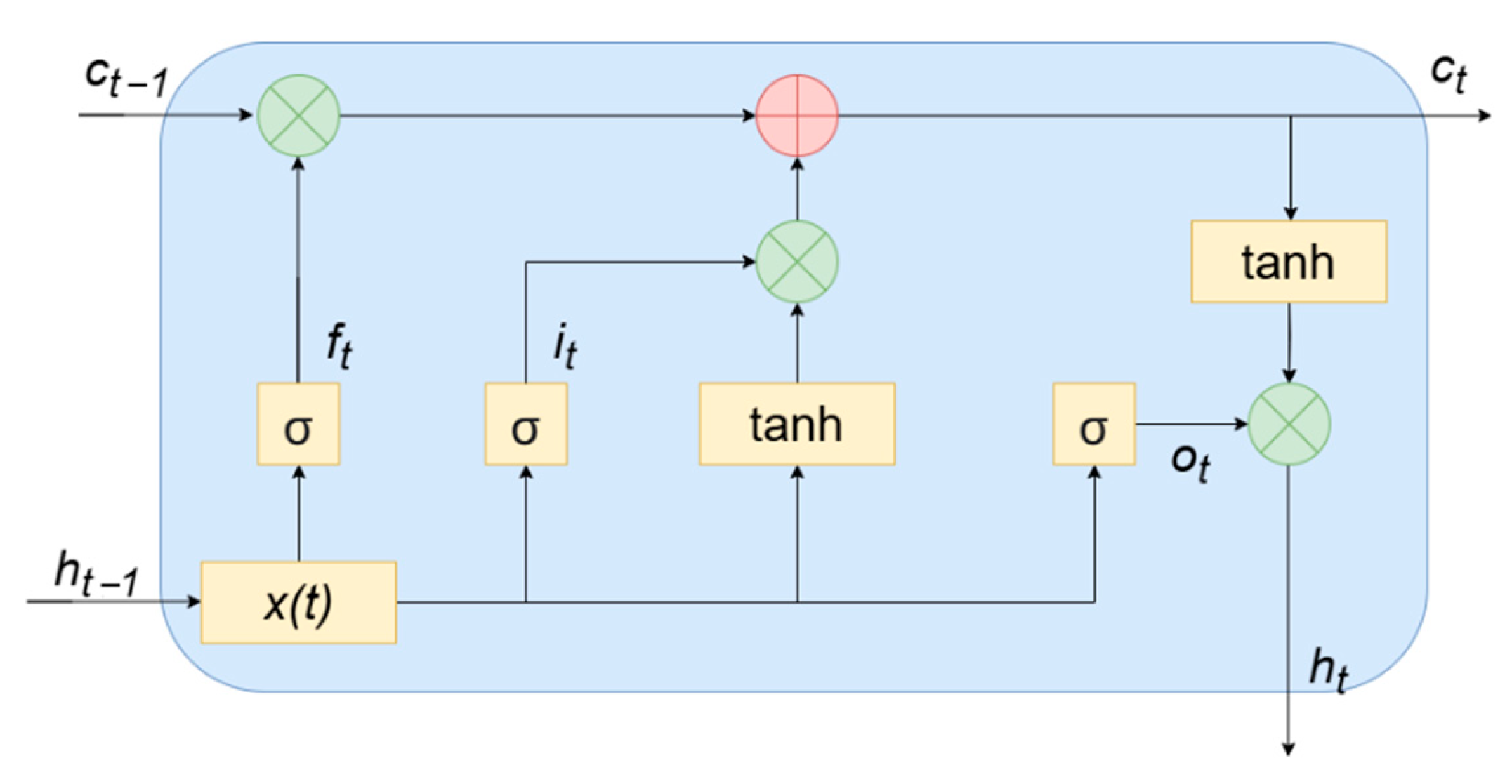
3.3. Long- and Short-Term Memory Networks
Long Short-Term Memory (LSTM) [
25] is a variant of Recurrent Neural Networks (RNNs), which enables the management of memory units by introducing special storage units and gate mechanisms to better capture long-term dependencies in sequential data.
The basic structure of LSTM is shown in
Figure 2. The LSTM cell contains the states of the memory cells as well as three gate control structures: forgetting gates, input gates, and output gates. The input forgetting gate performs selective forgetting, decides which information gets stored by computation, and acquires new cells by constantly updating the computation.
In
Figure 2,
,
are the hidden layer vectors at the time
and the time
, respectively;
,
are the cell states at the time
and the time
, respectively;
is the input at the time
;
is the Sigmoid activation function, with the value domain of [0, 1]; and tanh is the hyperbolic tangent activation function, with the value domain of [−1, 1]. The formulas for the input gate, forget gate and output gate are shown below.
where
,
is the weight assigned to the input gate;
is the bias of the input gate;
,
is the weight assigned to the forget gate;
is the bias of the forget gate;
,
is the weight assigned to the output gate; and
is the bias of the output gate.
The metameric state is updated at time
. The state is computed as
Candidates for the new cell state information store are
where
,
is the weight assigned to the candidate representative; and
is the bias of the candidate representative.
The implicit layer state at the time output is computed as
3.4. ISAO-Optimized LSTM
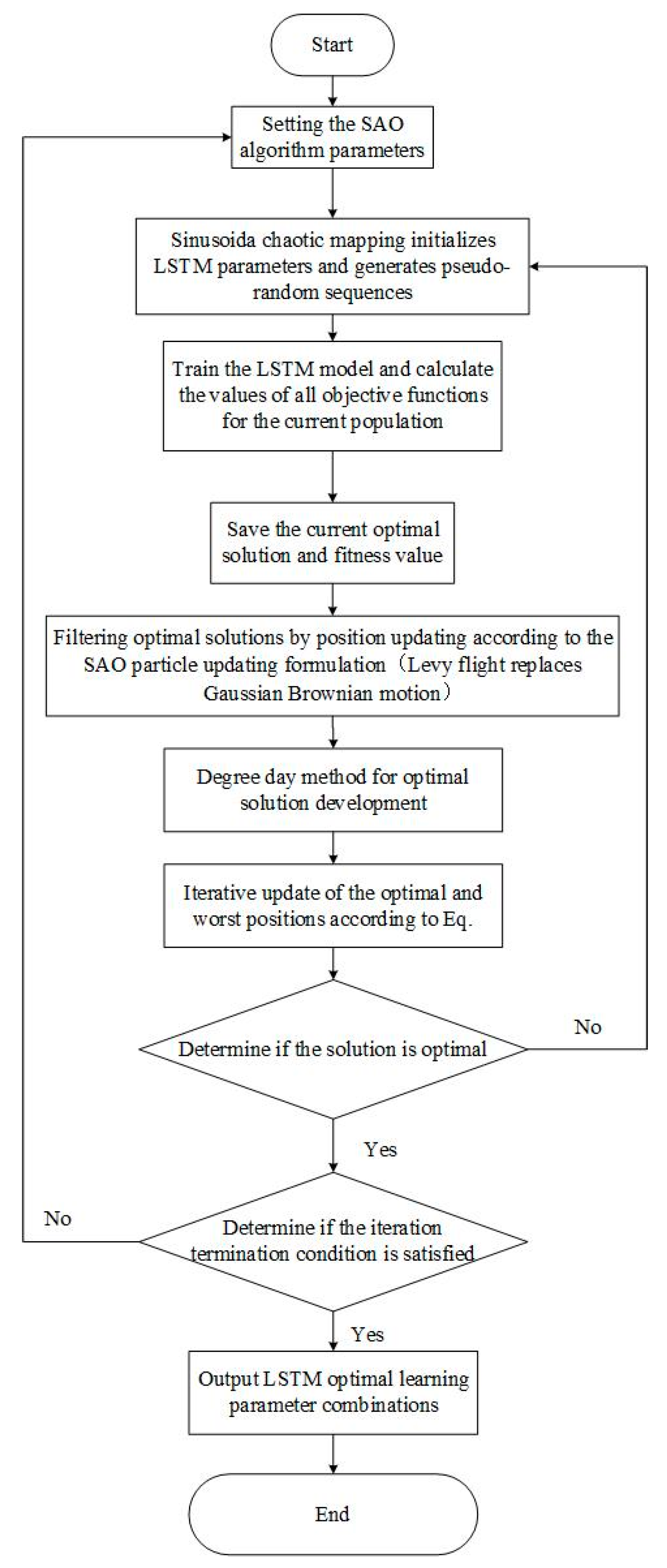
There are difficulties in the selection of certain hyperparameters in LSTM, and the correct selection of hyperparameters often affects the overall prediction accuracy. Traditional methods usually learn the parameters initially and cross-validate them based on experience. In this study, we used the ISAO algorithm to optimize the parameters of LSTM, adaptively search for appropriate neural network parameters, reduce the difficulty of learning and prediction, and improve the accuracy of prediction.
The ISAO learning parameter optimization process for LSTM is shown in
Figure 3.
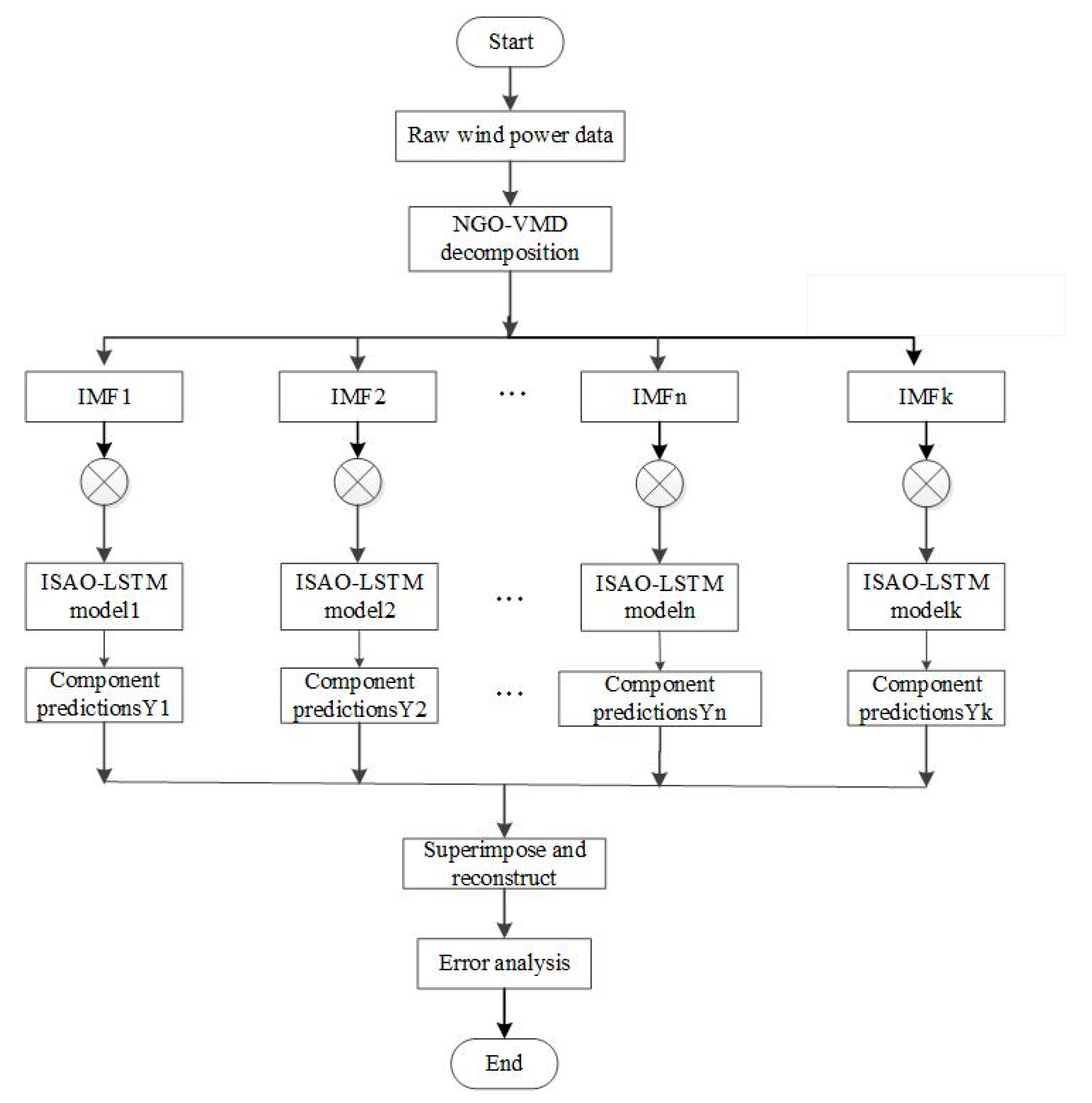
3.5. NGO-VMD-ISAO-LSTM Combined Prediction Model Building
This study combines the NGO optimization algorithm, VMD modal decomposition technique, ISAO optimization algorithm and LSTM prediction model to build the combined NGO-VMD-ISAO-LSTM model, and the specific steps are as follows:
- (1)
The NGO algorithm optimizes the VMD parameters [k,α], enabling the decomposition of raw wind power data into multiple subsequences using the enhanced VMD method;
- (2)
An ISAO-LSTM prediction model is constructed for each IMF component obtained from the decomposition. The ISAO algorithm adaptively tunes the neural network’s hyperparameters, thereby enhancing forecasting accuracy;
- (3)
The total prediction result is obtained by superposition reconstruction;
- (4)
Appropriate indicators are selected to analyze the errors.
The flow chart of NGO-VMD-ISAO-LSTM prediction is shown in
Figure 4.
3.6. Evaluation Indicators
To evaluate the forecasting performance of the proposed model, three key metrics were selected. Their calculation formulas are as follows
4. Simulation Analysis
The data used in this paper were collected over a 10-day period from 25 September to 5 October 2021 at a wind farm in Ningxia, China. The wind power data were sampled at 15 min intervals, resulting in a total of 1056 sets of data. Wind speed, wind direction, temperature and pressure were selected as input features. The first 80% of the data was selected as the training set and the remaining 20% as the test set, and the prediction time span was 45 h. Because wind power data are often affected by problems such as weather conditions and equipment failures, which can adversely affect the subsequent modeling decision-making process, the collected data were preprocessed accordingly. In this study, a combination of linear interpolation and forward/backward padding was used: for smooth trends with little variation, linear interpolation usually provides smoother and more reasonable padding; for data with large variations or no obvious trends, forward or backward padding can be considered, especially when missing values are at the beginning or end of the data. These methods can effectively fill in any gaps in the data to ensure data integrity and continuity.
In this study, the hardware equipment used for the wind power prediction experiment included an Nvidia GeForce RTX 4090 model graphics card, an i9-13900k model CPU, etc., and the software platform used was MATLAB2022B version.
4.1. Analysis of Single LSTM Model Prediction Results
To demonstrate the advantages of the LSTM prediction model proposed in this paper over other individual models in short-term wind power forecasting, ablation experiments were conducted using BP neural networks and Convolutional Neural Networks (CNN). The performance metrics for each model are presented in
Table 1.
As shown in
Table 1, the LSTM model achieved lower RMSE and MAE values compared to the BP and CNN models, reflecting a noticeable improvement in prediction accuracy. This suggests that the LSTM model is better suited to handling wind power data with pronounced temporal characteristics. The forecasting results of each model are illustrated in
Figure 5.
Figure 5 illustrates that, despite initial preprocessing, the non-stationary nature of wind power data still causes discrepancies between predicted and actual values at certain points, negatively impacting model fitting. Due to these challenges, relying solely on a single prediction model is insufficient. Therefore, the VMD algorithm was employed to decompose the data and reduce noise. Additionally, to address the difficulty in selecting LSTM hyperparameters and enhance prediction accuracy, the ISAO algorithm was introduced for hyperparameter optimization.
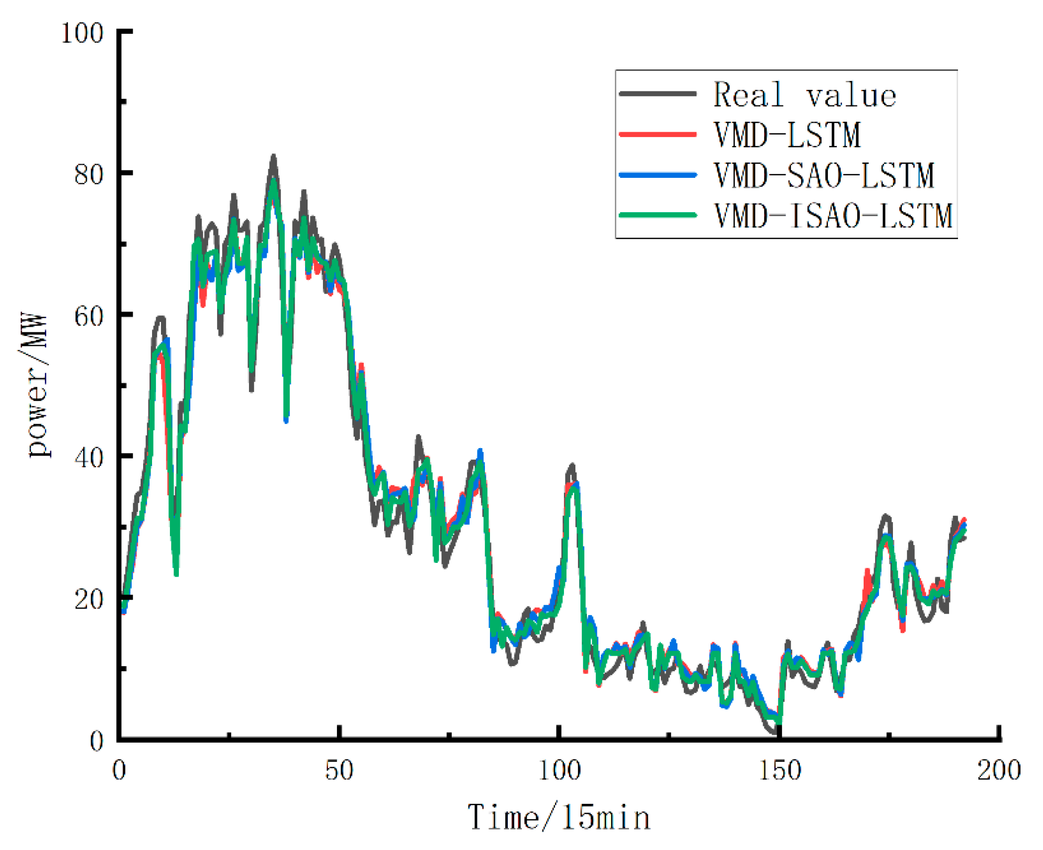
4.2. Analysis of VMD-SAO-LSTM Model Prediction Results
In order to verify the performance of the VMD-SAO-LSTM model, three models, VMD-LSTM, VMD-SAO-LSTM and VMD-ISAO-LSTM, were selected for the comparison of the prediction results. The sampling frequency of the VMD was 1000 Hz, the modal number of the center frequency rule of thumb was six, and the penalization factor α was adjusted to 3000 according to the smoothness of the signals. The convergence tolerance criterion was 10–7 with no DC part. The VMD decomposition results are shown in
Figure 6.
Both SAO and ISAO use a population size of 10, 30 iterations, and a degree-day factor of 0.35. These algorithms adaptively optimize the LSTM model’s initial learning rate, hidden unit count, and L2 regularization parameter. The evaluation metrics for each combined prediction model are presented in
Table 2.
Combined with
Table 2, it can be seen that after the introduction of VMD decomposition technology and the SAO optimization algorithm, all evaluation indexes were significantly improved. Specifically, the ISAO optimization algorithm improved RMSE and MAE by 5.1% and 6.8%, respectively, compared to the SAO optimization algorithm, which proves the feasibility of applying VMD decomposition technology and the ISAO optimization algorithm in the field of wind power prediction. The prediction results of each combined prediction model are shown in
Figure 7.
Figure 7 shows that most predicted points closely follow the actual wind power trends. However, because VMD parameters are manually set and not adaptive, prediction efficiency is limited. To address this, this study introduced the NGO optimization algorithm to adaptively optimize VMD hyperparameters, identifying the best combination of modal number and penalty factor to enhance prediction accuracy.
4.3. Analysis of the Prediction Results of the NGO-VMD-SAO-LSTM Model
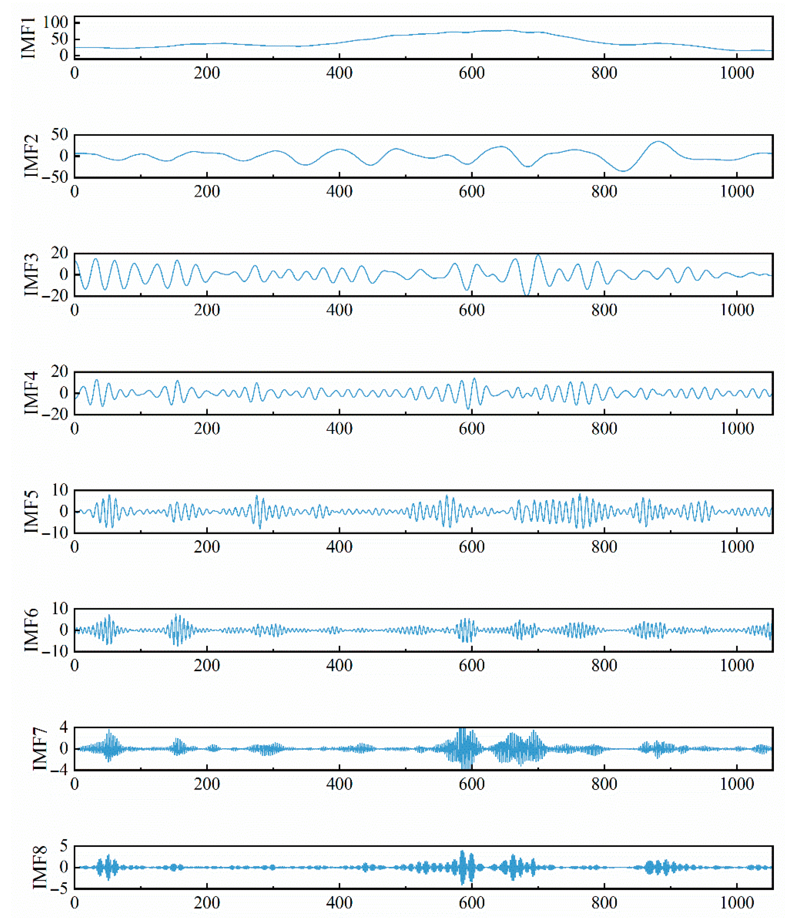
The VMD parameters, including sampling frequency, were set as described, while the optimal modal number and penalty factor were determined through NGO optimization. The NGO algorithm uses a population size of 10 and runs for a maximum of 30 iterations. Using minimum arrangement entropy as the fitness function, NGO adaptively finds the best combination of modal number and penalty factor—resulting in eight modes and an α value of 2867. The decomposition results of NGO-VMD are shown in
Figure 8.
Figure 8 shows that the NGO-VMD model decomposed the original sequence into eight subsequences. IMF1 and IMF2, as the primary modes, exhibit smoother curves; IMF3, IMF4, and IMF5 are roughly symmetric, easing prediction difficulty; while IMF6, IMF7, and IMF8 capture the overall volatility of the wind power series. Compared to the single VMD decomposition shown in
Section 3.2, these eight components are more regular and better capture the original series’ features. This demonstrates that incorporating NGO optimization improves VMD’s ability to preserve data characteristics and reduce modal aliasing, providing a stronger foundation for accurate prediction.
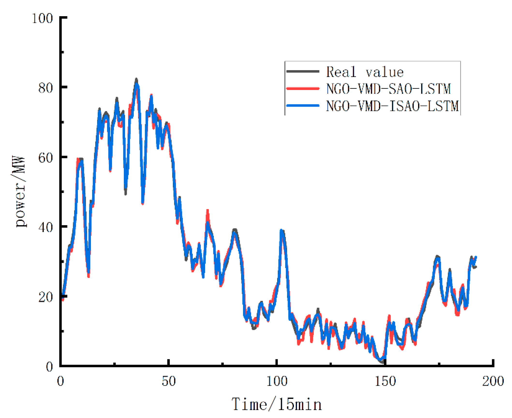
The prediction results based on the NGO-VMD-ISAO-LSTM prediction model and the comparison model are shown in
Figure 9, and the corresponding evaluation indexes are shown in
Table 3.
Compared to the NGO-VMD-SAO-LSTM model, the NGO-VMD-ISAO-LSTM achieved improvements of 13.64%, 18.51%, and 0.5% in RMSE, MAE, and RMSE. Among all the models discussed in
Section 3.1 and
Section 3.2, the proposed model exhibited the lowest prediction error and highest accuracy, further demonstrating its effectiveness and reliability for short-term wind power forecasting.


