Structural Health Prediction Method for Pipelines Subjected to Seismic Liquefaction-Induced Displacement via FEM and AutoML

Abstract

This study investigates the mechanical behavior and safety performance of buried natural gas pipelines crossing seismically active fault zones and liquefaction-prone areas, with particular application to the China–Russia East-Route Natural Gas Pipeline. The research combines experimental testing, numerical simulation, and machine learning to develop an advanced framework for pipeline safety assessment under seismic loading conditions. A series of large-scale pipe–soil interaction experiments were conducted under seismic-frequency cyclic loading, leading to the development of a modified soil spring model that accurately captures the nonlinear soil-resistance characteristics during seismic events. Unlike prior studies focusing on static or specific seismic conditions, this work uniquely integrates real cyclic loading test data to develop a frequency-dependent soil spring model, significantly enhancing the physical basis for dynamic soil–pipeline interaction simulation. Finite element analyses were systematically performed to evaluate pipeline response under liquefaction-induced ground displacement, considering key influencing factors including liquefaction zone length, seismic wave frequency content, operational pressure, and pipe wall thickness. An innovative machine learning-based predictive model was developed by integrating LightGBM, XGBoost, and CatBoost algorithms, achieving remarkable prediction accuracy for pipeline strain (R² > 0.999, MAPE < 1%). This high accuracy represents a significant improvement over conventional analytical methods and enables rapid safety assessment. The findings provide robust theoretical support for pipeline routing and seismic design in high-risk zones, enhancing the safety and reliability of energy infrastructure.

1. Introduction

Natural gas, as a critical component in the national energy structure transition, has drawn significant attention regarding its transportation safety. In seismically active and liquefaction-prone regions, earthquake-induced ground displacements impose substantial damaging effects on buried pipelines. Therefore, conducting in-depth research on pipeline response mechanisms under seismic liquefaction-induced displacement, elucidating the distribution patterns of mechanical responses, and developing high-precision predictive models for pipeline strain under such conditions hold substantial engineering significance for ensuring the safety of oil and gas transportation infrastructure.

The seismic effects on underground pipeline systems have long been a focal point in geotechnical and structural engineering research. In 1988, Kamel et al. [1] modeled the pipeline as a continuous beam supported by soil springs. This approach more effectively simulated the interaction between the soil and the pipeline during seismic events. This method takes into account the nonlinear characteristics of the soil springs as well as the nonlinear behavior of the pipeline itself, thereby being able to describe the dynamic response of the pipeline more comprehensively. Zhang Jinguo et al. [2] derived finite element equations for pipeline structural responses under seismic loading, providing a theoretical basis for more accurately describing pipeline behavior under seismic fault dislocation. Through two-dimensional finite element modeling, Guo Endong et al. [3,4] gained in-depth understanding of pipeline responses under consistent displacement conditions across active faults. Such research not only helps reveal the seismic response mechanisms of pipeline structures in complex geological environments but also provides valuable references for related engineering design and construction. Hindy et al. [5] emphasized the effects of random seismic excitation on pipelines, finding that random earthquakes could induce excessive stresses whose severity correlates with the spatial coherence and frequency content of seismic excitation. Through site microtremor measurements and spectral analysis, Xu Jiancong et al. [6] concluded that thick soft soil layers have a certain amplification effect on microtremors. Regarding soil liquefaction induced by earthquakes, numerous scholars have conducted investigations. Madabhushi et al. [7] employed dynamic finite element methods to simulate the response of rectangular cross-section tunnels under liquefied ground conditions caused by earthquakes. Azadi et al. [8] focused particularly on analyzing the effects of seismic-induced soil liquefaction on tunnel stability, paying special attention to the trends of buoyant displacement. Using shaking table tests, Tang Aiping et al. [9] simulated the response of utility tunnel systems and surrounding soils under seismic conditions, preliminarily exploring the behavioral characteristics of entire utility tunnel systems during earthquakes. Reza Saeedzadeh et al. [10] conducted a finite element analysis to investigate the upward response of buried pipelines in saturated sandy soil under seismic loads. They found that the pipeline burial depth and the sand density ratio had a significant impact on the upward movement, and there was an optimal groundwater-level drop that could reduce the risk of upward movement. Kongming Yan et al. [11] conducted large-scale vibration test model experiments to investigate the seismic response of deeply buried pipelines under non-uniform excitation. They measured and analyzed the pipeline strain, displacement, and soil acceleration, and found that the non-uniform excitation had a significant impact, and the pipeline exhibited three-dimensional movements such as rotation. However, most existing studies focus on pipeline stress states under specific seismic conditions, lacking tools for rapid numerical simulation of soil–pipeline interaction that can accurately reflect the quantification methods for soil ultimate resistance under dynamic seismic loads with frequency characteristics. Research on pipeline strain prediction methods based on true soil–pipeline interaction under seismic conditions also remains unexplored.

To address these critical issues, this study conducts experimental investigations on pipe–soil interaction under seismic loading, grounded in practical engineering contexts. This study proposes a frequency-modified soil spring model specifically adapted for seismic conditions, and performs comprehensive parametric simulations of pipeline response. The research route is shown in Figure 1. Through these efforts, this study establish a strain data-driven optimal prediction model for pipeline safety assessment, providing theoretical support for enhancing the design reliability of buried pipelines in earthquake-prone regions.

2. Experimental Investigation of Soil–Pipeline Interaction Under Seismic Loading

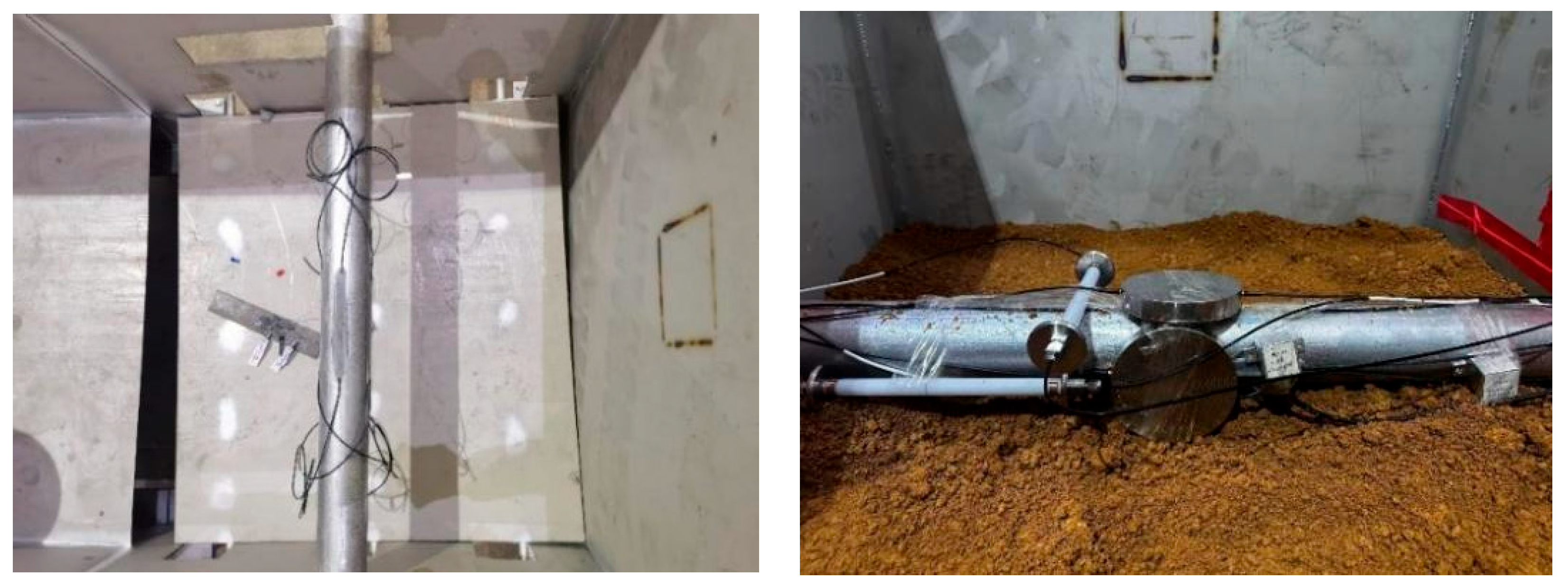
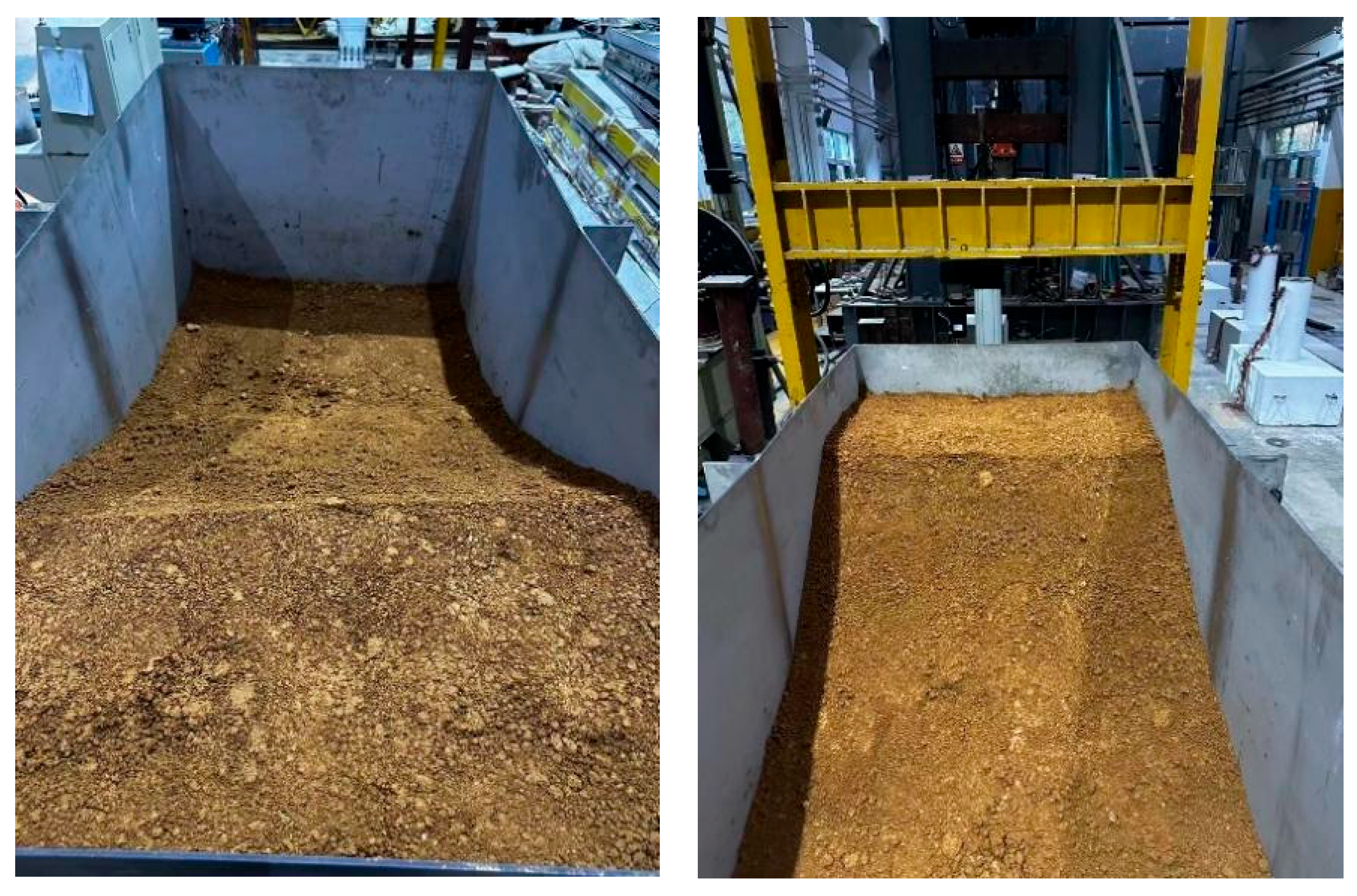
2.1. Soil–Pipeline Interaction Test Platform

This test bench is capable of conducting vibration tests (0–20 Hz frequency range, 200 mm working stroke) and sweep-frequency vibration tests in a laboratory environment. It is suitable for structures weighing up to 5000 kg and can load time–history seismic waves to simulate earthquake vibrations. The system is equipped with a multi-channel data acquisition system and a vibration testing and analysis system for collecting and analyzing multi-channel structural data during experiments.

Figure 2 shows the layout of the test setup, including the integrated steel frame soil container with L-shaped sliding channels (0–400 mm displacement range) and retractable soil-retaining plates to prevent leakage during pipeline movement. Figure 3 shows the display of the test device after it has been installed.

2.2. Soil Parameters

Direct shear tests were conducted on typical soft soils from the China–Russia East-Route Pipeline region. Four specimens were tested under different normal stresses, with horizontal shear forces applied until failure. The shear stress at failure was measured, and the soil’s shear strength parameters—internal friction angle (φ) and cohesion (c)—were determined based on Coulomb’s failure criterion.

Soil density was measured using ring-sampling methods, with two replicates per soil type. The average value was adopted as the final density (see

Table 1. Soil parameters.

Soil Sample	Density/(kg/m3)	Cohesion/KPa	Internal Friction Angle/°
Soft Clay	1531	34	22.5
Stiff Clay	2100	44	27.0

for parameters).

2.3. Experimental Procedure and Analysis

For dynamic loading, sinusoidal acceleration waves (1–5 Hz, 5 cm peak displacement) were applied simultaneously along both horizontal directions (Figure 4). Figure 4A–F respectively present shaking table response spectra for seismic frequencies of 0–5 Hz, selected based on their controllability and capacity to simulate seismic wave characteristics.

The soil pressure responses under different loading conditions during horizontal seismic wave excitation are presented in Figure 5. In Figure 5A–F show the load-displacement curves of two types of soil with seismic frequencies ranging from 0 to 5 Hz. As shown in Figure 5, when seismic waves propagate horizontally, both soft and stiff soils generally exhibit a characteristic trend of initial increase followed by decrease in maximum stress response with increasing frequency. At low frequencies (1 Hz and 2 Hz), the peak stress responses for both soil types remain relatively low. The stress responses reach their maximum values at intermediate frequencies (3 Hz and 4 Hz), followed by a slight decrease at 5 Hz. This observed pattern may be attributed to the resonant behavior of soils, where intermediate-frequency dynamic loading is more likely to induce resonance effects, consequently resulting in amplified stress responses.

The stress response of stiff soil consistently exceeds that of soft soil across all frequencies, particularly at peak positions. This observation indicates that the relatively higher stiffness and lower damping characteristics of stiff soil lead to more pronounced stress responses, whereas soft soil exhibits greater damping effects, resulting in comparatively smaller stress responses. With increasing frequency, the stress response of soft soil gradually stabilizes, while stiff soil continues to demonstrate significant stress variations. This phenomenon suggests that the plastic behavior of soft soil tends to dissipate energy more effectively under high-frequency dynamic loading, consequently reducing stress responses.

At lower frequencies (e.g., 1 Hz), the displacement curves exhibit relatively smooth profiles with delayed peak stress occurrence, demonstrating a distinct hysteresis effect where soil deformation and stress development proceed more gradually. Under intermediate to high frequencies (3 Hz and 4 Hz), both displacement and stress peaks emerge earlier, accompanied by steeper stress growth rates. This behavior reflects accelerated internal stress responses and diminished hysteresis effects in soils subjected to higher frequency loading.

Collectively, the frequency-dependent stress responses of soils demonstrate complex trends with differential sensitivity between soft and stiff soils. Lower frequencies produce smaller stress responses, while intermediate frequencies (particularly around 3–4 Hz) generate significantly amplified responses, reaching maximum stress peaks. These findings highlight the crucial influence of soil type and loading frequency on dynamic soil behavior, with stiff soils showing greater stress amplification and soft soils exhibiting enhanced energy dissipation characteristics under varying frequency conditions.

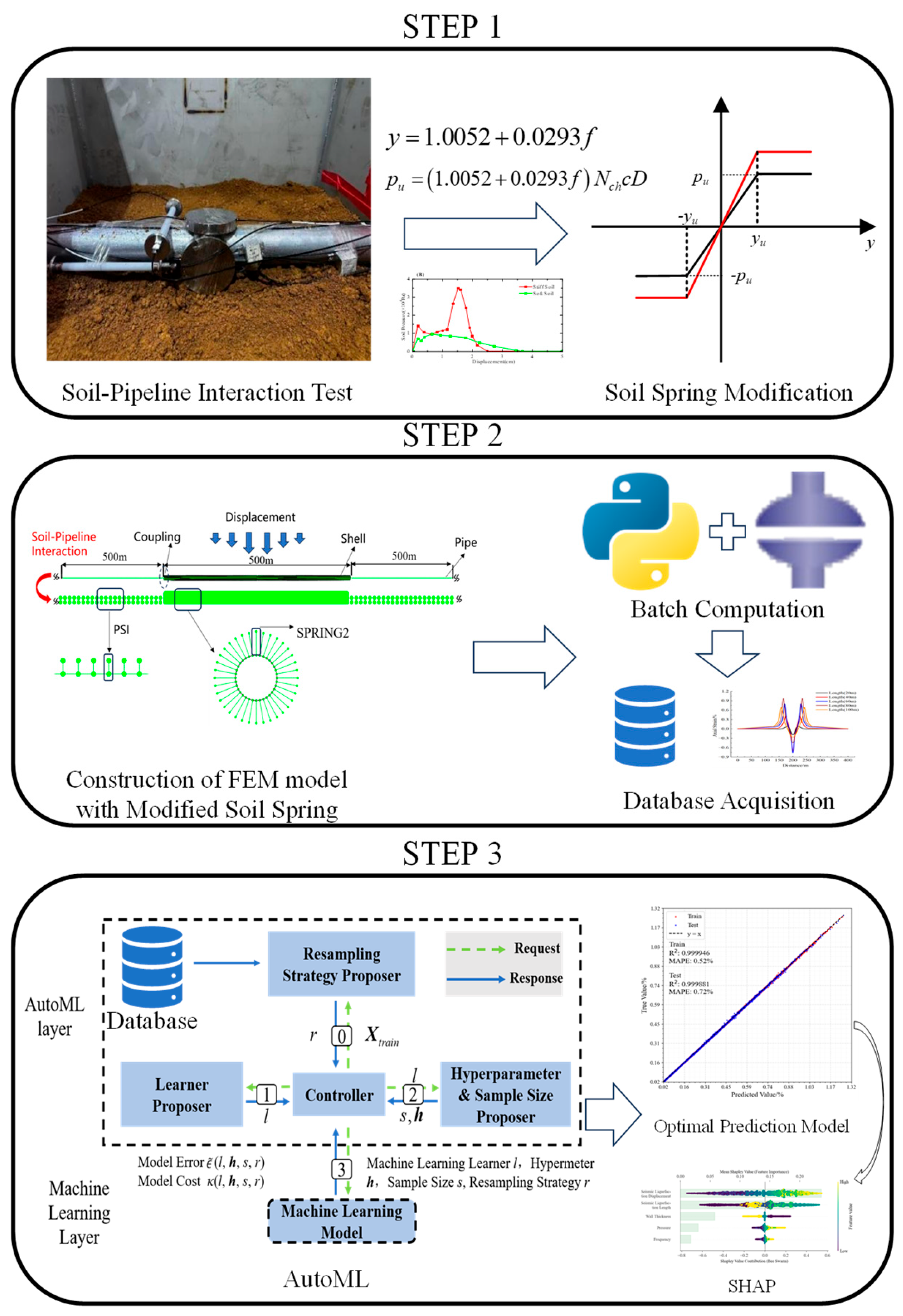
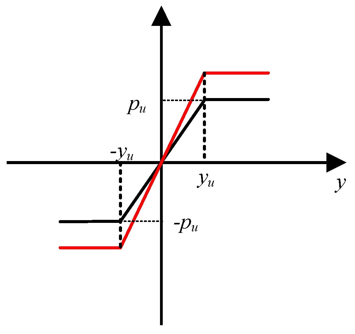
2.4. Soil Spring Modification

Considering the predominantly clayey soil conditions along the China–Russia Eastern Pipeline route, the modified soil spring model exclusively addresses clay behavior. Adopting a conservative approach, the revised soil spring model maintains the bilinear horizontal configuration illustrated in Figure 6, with modifications applied solely to the soil’s ultimate resistance. The black line represents the constitutive model of the original soil spring, while the red line denotes the modified soil spring constitutive model. Through regression analysis of experimental data obtained from two clay types under various loading conditions, we incorporated the predominant frequency of seismic motion to develop a modified formulation for horizontal soil springs. Equation (1) presents the analytical clay formula originally provided in ASCE-ALA (2001) [10].

Table 2. Relative amplification factors under horizontal dynamic loading at different frequencies.

Frequency (Hz)	Relative Amplification Factor
0	1.0
1	1.0376
2	1.0702
3	1.0901
4	1.1216
5	1.1505

displays the relative amplification coefficients corresponding to different frequencies of dynamic loading. Figure 7 displays the fitted straight line obtained through regression analysis. Notably, the horizontal soil spring formulation in Equation (1) remains valid solely for static loading scenarios. By performing linear regression, a straight line was fitted as shown in Figure 7. We established the relationship between input seismic frequency and relative amplification coefficient, as expressed in Equation (2). Consequently, the modified lateral soil spring formulation emerges as Equation (3).

$$p_u=N_{ch}cD$$

(1)

where $p_u$ represents ultimate soil resistance, kN/m, N_ch represents the clay-bearing capacity factor, c denotes soil cohesion, kPa, and D signifies the pipe diameter, m.

$$y=1.0052+0.0293f$$

(2)

$$p_u=\left(1.0052+0.0293f\right)N_{ch}cD$$

(3)

3. Mechanical Response of Buried Pipelines Subjected to Seismic Liquefaction-Induced Displacement

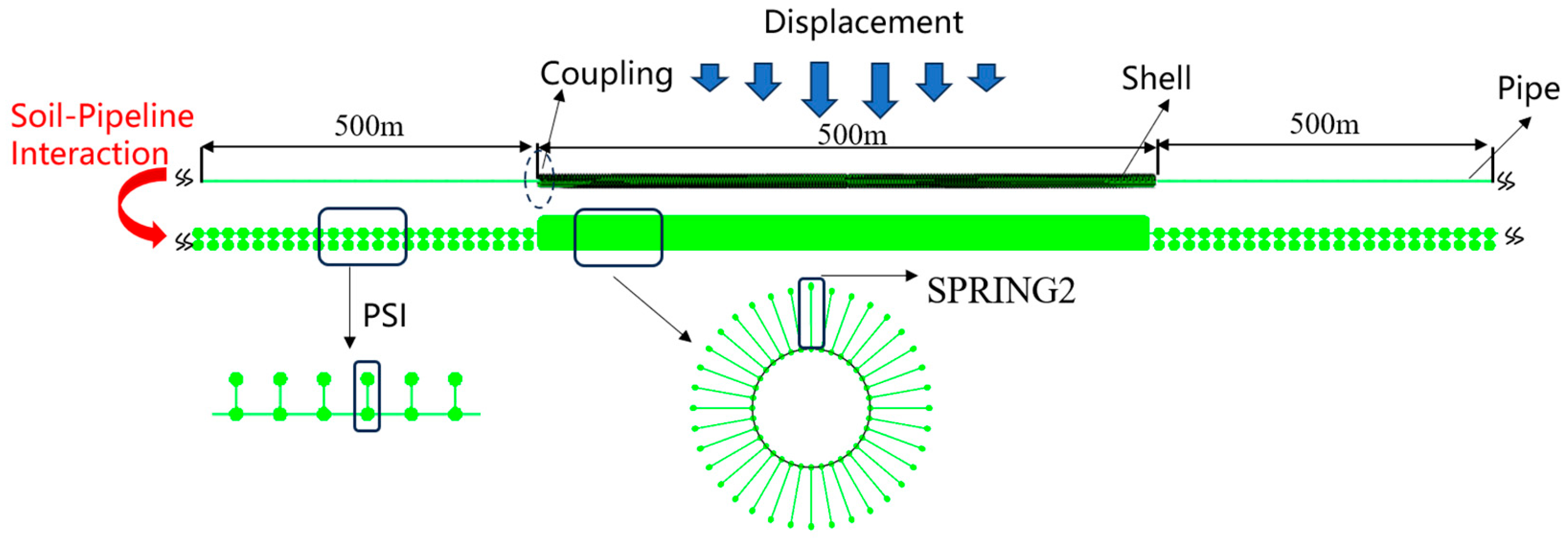
3.1. Nonlinear Soil–Pipeline Interaction Model

This study conducted finite element analysis based on ABAQUS. Given that traditional pipeline elements are difficult to simulate local deformation, and shell elements have high computational costs, a pipe–shell coupling model was constructed: for the X80 pipeline, the 500 m sections at both ends used the PIPE31 element, and the sliding slope section was precisely depicted using 40 circumferential divided S4R shell elements to simulate deformation. Distributed coupling constraints were applied at the connection between the pipe and the shell to bind degrees of freedom and avoid the stress concentration problem caused by multi-point coupling [12]. Soil nodes were set on the periphery of the shell elements, and the pipe–soil interaction was simulated using the nonlinear SPRING2 element to describe the three-dimensional soil spring constraint relationship. The finite element model of the interaction between the pipeline and the soil is shown in Figure 8. This model integrates linear cross-sectional elements, shell elements, advanced coupling constraints, and three-dimensional soil constraints to achieve a unified balance between computational efficiency and result reliability.

3.2. Selection of Model and Computational Case Parameters

3.2.1. Pipeline Parameters

In numerical calculations, the actual stress–strain curve of the pipeline material must be employed. The corresponding material curve is selected for computation in accordance with Seismic Technical Code for Oil and Gas Transmission Pipeline Engineering (GB/T 50470-2017) [13]. For the China–Russia Eastern Pipeline constructed with X80 steel, the stress–strain curve of the pipeline steel is derived using the standard-specified formulas, as illustrated in Figure 9.

3.2.2. Soil Spring Parameters

Based on the soil parameters described in Section 2.2, soft clay was selected as the representative soil condition. For the China–Russia Eastern Pipeline with a diameter of 1422 mm, the burial depth was set at twice the pipe diameter (2D) as the typical installation condition. The ultimate soil resistance was determined using the modified soil spring model, while the ultimate soil displacement was calculated according to the recommended formula in ASCE-ALA (2011) [10]. The parameters of lateral soil springs under different frequency conditions are presented in

Table 3. Soil spring parameters.

Frequency	Lateral Soil Springs
	Soil Force/(kN/m)	Ultimate Displacement/mm
0 HZ	285.1	140.4
1 HZ	295.8	140.4
2 HZ	305.1	140.4
3 HZ	310.8	140.4
4 HZ	319.8	140.4
5 HZ	328.0	140.4

. The remaining soil spring parameters were specified as follows: Axial soil spring: ultimate resistance is 156.2 kN/m, ultimate displacement is 10 mm; Vertical upward soil spring: ultimate resistance is 190.4 kN/m, ultimate displacement is 28.4 mm; Vertical downward soil spring: ultimate resistance is 843.9 kN/m, ultimate displacement is 28.4 mm.

3.2.3. Calculation Conditions

This study performed numerical simulations targeting the China–Russia Eastern Pipeline, where the parameter selection incorporated typical values encompassing four key variables: liquefaction zone length, seismic wave frequency, internal pipeline pressure, and pipe wall thickness. The computational matrix comprised 630 distinct working conditions with a maximum displacement of 4 m, during which both the maximum and minimum axial strains were systematically recorded at 0.2 m intervals, ultimately yielding 13,230 comprehensive datasets as detailed in

Table 4. Selection of computational case parameters.

Names
Length of Liquefaction Zone (m)	Seismic Wave Frequency (Hz)	Internal Pipe Pressure (MPa)	Pipe Wall Thickness (mm)
20	0	0	21.4
40	1	2	25.7
60	2	4	30.7
80	3	6
100	4	8
	5	10
		12

. The baseline working condition was established with specific parameters including a 60 m liquefaction zone length, 3 Hz seismic wave frequency, 12 MPa internal pipeline pressure, and 25.7 mm pipe wall thickness. For subsequent comparative analyses examining individual influencing factors, all remaining parameters were consistently maintained at these baseline values to ensure methodological rigor in isolating variable-specific effects. This analytical approach enabled thorough investigation of pipeline response characteristics under various seismic loading scenarios while maintaining controlled experimental conditions for precise parameter sensitivity assessment, with the extensive dataset providing robust statistical significance for evaluating pipeline performance under liquefaction-induced displacement conditions specific to the China–Russia Eastern Pipeline project.

Key assumptions in the FEM simulations include: (1) homogeneous soil properties within the liquefaction zone, (2) application of the Suzuki displacement pattern as a quasi-static representation of liquefaction-induced displacement, (3) linear elastic–perfectly plastic pipe material behavior beyond yield, and (4) neglect of inertial effects and wave propagation within the pipe during the displacement event. These assumptions simplify the complex dynamic problem to focus on the dominant displacement-controlled mechanism but limit the direct applicability to high-frequency shaking scenarios. Limitations include the reliance on a specific displacement pattern and the focus on clayey soils; sandy liquefaction behavior may differ significantly.

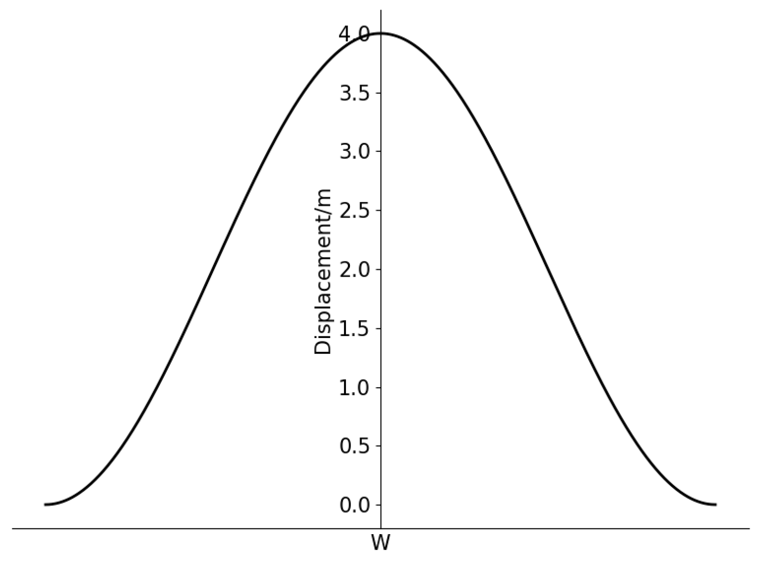
3.3. Liquefaction-Induced Displacement

One of the primary indicators for evaluating pipeline response under seismic liquefaction-induced lateral displacement is the ground deformation pattern, which describes the variation of ground displacement across the width of the liquefaction zone. In this study, the soil liquefaction displacement characterization method proposed by Suzuki et al. was adopted, expressed as Equation (4) [14]. The maximum displacement was assumed to be 4 m, and the applied lateral displacement loading pattern is illustrated in Figure 10.

$$y(x)=\delta \cdot {(\cos {\displaystyle \frac{\pi x}{W}})}^n$$

(4)

where W represents the distance between the two boundaries of the displacement zone, m; $x$ indicates the non-normalized distance from the center line of the displacement zone, m; and n is assigned a value of 2 as the shape parameter governing the displacement profile.

4. Analysis of Influencing Factors on Pipeline Mechanical Response

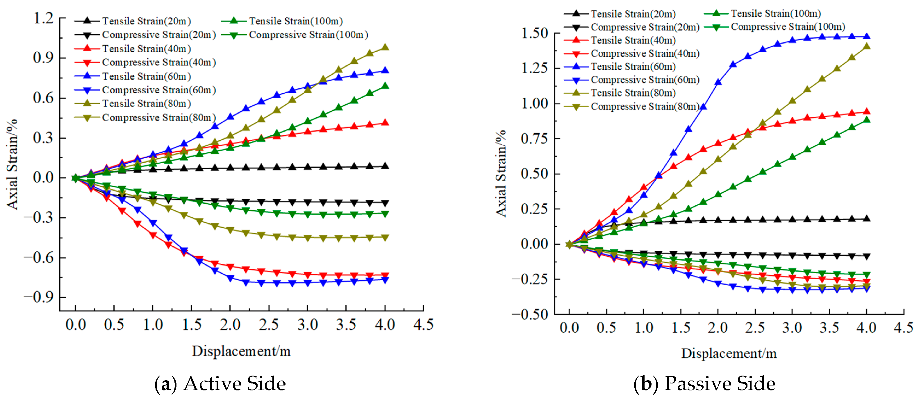
4.1. Length of Liquefaction Zone

The length of the seismic liquefaction zone constitutes a critical geological parameter influencing the mechanical response of buried pipelines. As evidenced in Figure 11 and Figure 12, both axial tensile and compressive strains at the pipeline mid-section demonstrate an initial increase followed by subsequent reduction as the liquefaction zone length extends. This behavioral pattern stems from distinct mechanical mechanisms: for shorter liquefaction zones, pronounced constraint effects from adjacent non-liquefied regions impose significant “restrictive clamping” on pipeline deformation, resulting in relatively smaller axial strain magnitudes due to localized deformation. In contrast, extended liquefaction zones exhibit weakened boundary constraints while requiring the pipeline to accommodate larger-scale lateral ground displacements, consequently developing either free bending or tensile states that inevitably induce greater longitudinal deformation amplitudes and correspondingly elevated axial strain levels. When the zone length exceeds a critical threshold, the deformation curvature of the pipeline decreases, thereby reducing strain accumulation. During seismic loading, progressive strain accumulation facilitates the expansion of plastic deformation zones, ultimately forming stress–strain concentration regions that substantially compromise the pipeline’s overall seismic safety performance.

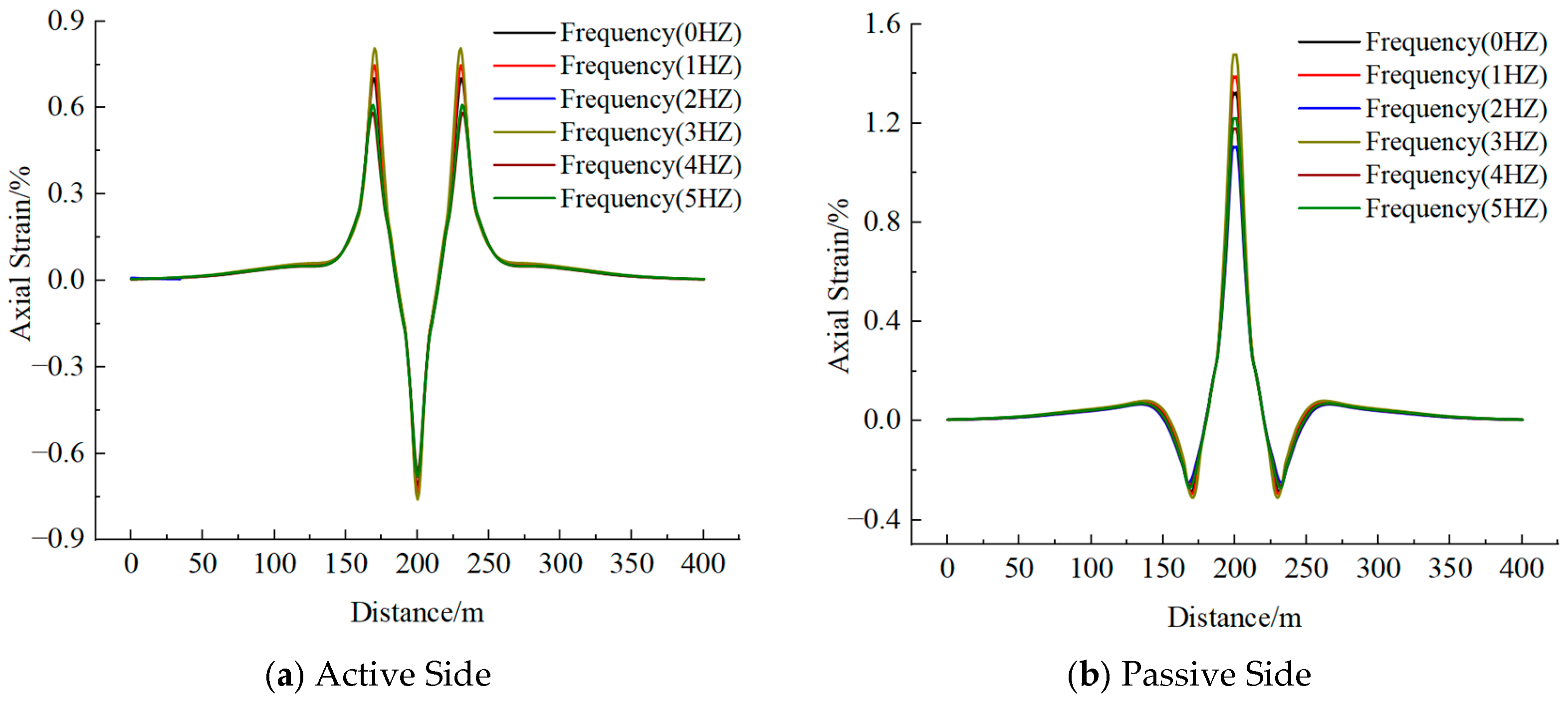
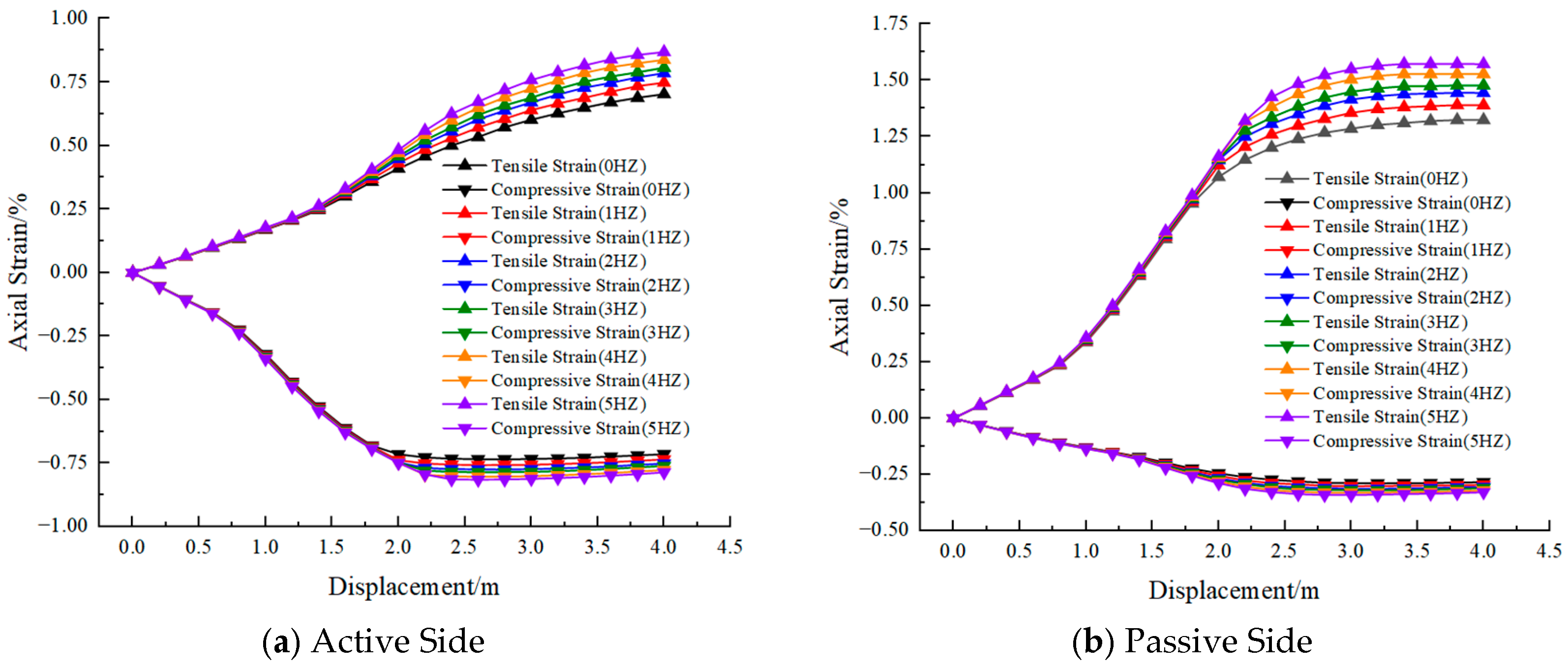
4.2. Seismic Wave Frequency

As illustrated in Figure 13 and Figure 14, seismic wave frequency exerts a non-negligible influence on pipeline axial strain evolution. The axial strain demonstrates a progressive increase with rising frequency, primarily attributed to corresponding enhancement in lateral soil spring ultimate resistance. When pipeline deformation reaches yield strength under sustained loading, strain variation exhibits abrupt changes. Consequently, the differential effects of various seismic frequencies become increasingly pronounced at larger displacement levels. However, as displacement continues to accumulate, the pipeline deformation gradually stabilizes, leading to eventual plateauing of maximum axial strain values.

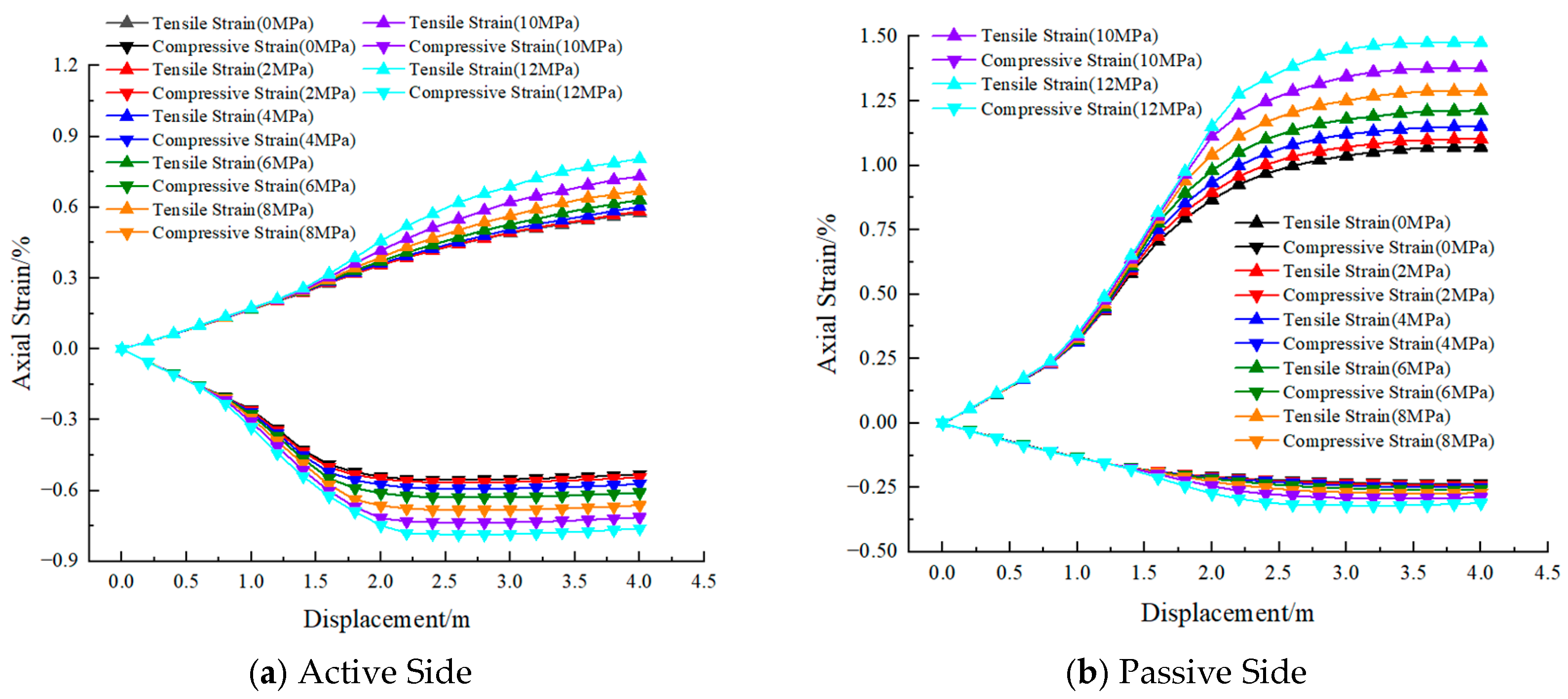
4.3. Internal Pipe Pressure

The internal pressure significantly alters the pipeline’s structural stiffness and deformation patterns, thereby profoundly influencing the evolution of axial strain. As demonstrated in Figure 15 and Figure 16, under low internal pressure conditions, the pipeline exhibits greater structural flexibility. While external liquefaction-induced displacements more readily induce overall axial tension or compression in such cases, the contribution of internal pressure to axial strain remains minimal, resulting in relatively lower total strain magnitudes. Conversely, elevated internal pressure conditions lead to substantially greater axial strains when combined with displacement effects, particularly at larger displacement levels where this phenomenon becomes more pronounced. Notably, regardless of internal pressure magnitude, since the initial axial strain condition remains zero, pipelines operating under higher internal pressures demonstrate accelerated axial strain accumulation rates during loading.

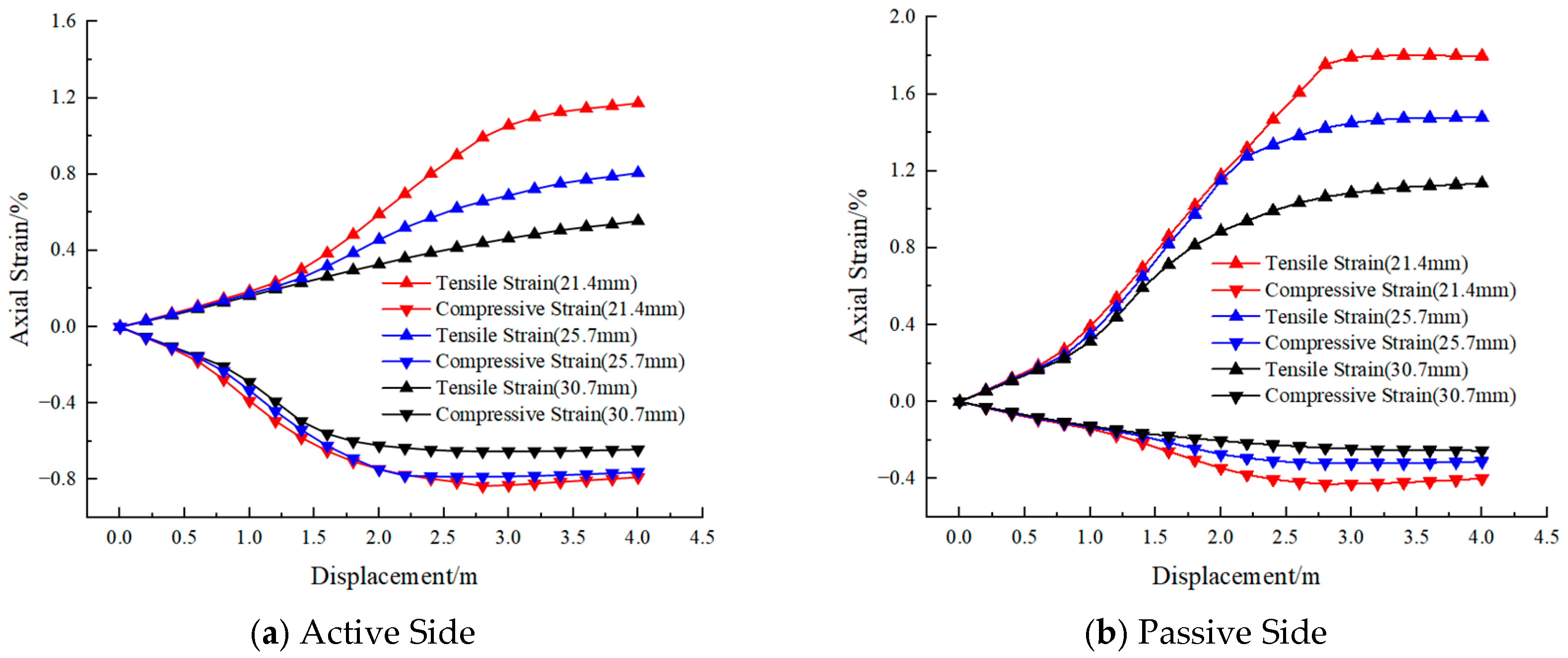
4.4. Pipe Wall Thickness

Analysis of the axial strain results presented in Figure 17 and Figure 18 reveals the significant controlling effect of wall thickness on tensile-compressive deformation. Thin-walled pipelines subjected to seismic liquefaction-induced shear displacement exhibit pronounced axial tension or compression, resulting in substantial axial strain amplitudes. In contrast, thick-walled pipelines demonstrate markedly enhanced axial stiffness, effectively mitigating structural deformation and substantially suppressing strain development under identical loading conditions. The strategic increase in wall thickness represents an effective approach to enhance deformation control in seismic design, particularly for high-grade steel pipelines or critical infrastructure. However, excessive wall thickness may lead to significant economic inefficiency. Consequently, optimal wall thickness should be carefully determined in design to achieve a balanced stiffness–flexibility relationship, ensuring coordinated seismic resistance while maintaining cost-effectiveness.

5. The Intelligent Prediction of Pipeline Structural Safety Under Seismic Liquefaction-Induced Displacement

In order to achieve real-time response analysis of pipeline structural safety under seismic liquefaction-induced displacement hazards, a safety state prediction database is developed based on a finite element mechanical model of pipelines subjected to such conditions. Leveraging automated machine learning (AutoML), the framework facilitates the automatic construction of optimal predictive models and the selection of optimal hyperparameters, thereby enabling the development of high-accuracy safety state prediction models.

5.1. Database Construction

To accurately predict the mechanical response and safety state of buried pipelines under co-seismic liquefaction-induced landslide displacement, a database of maximum and minimum axial strains on the active and passive sides of the pipeline under landslide loading is constructed. The input parameters of the database are shown in

Table 5. Input parameters of the pipeline mechanical response database under seismic liquefaction.

Pipe Diameter/mm	Wall Thickness/mm	Seismic Liquefaction Length/m	Pressure/MPa	Frequency/Hz	Seismic Liquefaction Displacement/m
1422	21.4, 25.7, 30.7	20, 40, 60, 80, 100	0~12	0~5	0~4.0

.

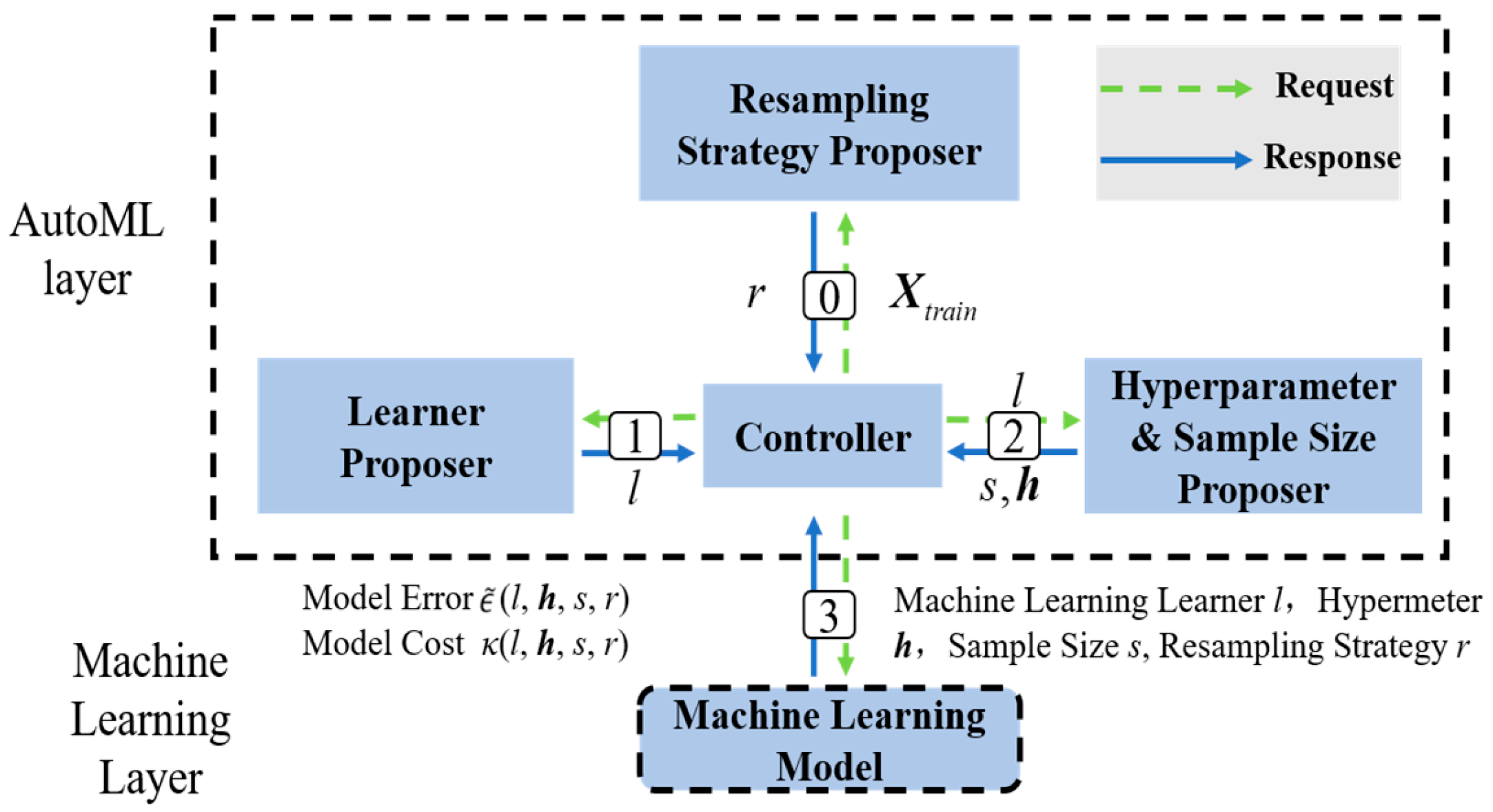
5.2. Machine Learning Algorithms

To improve the accuracy of axial strain prediction in pipelines subjected to seismic liquefaction, modern machine learning models require extensive hyperparameter tuning, which is complex and computationally demanding. To address this, researchers have introduced Automated Machine Learning (AutoML) to automate model selection and hyperparameter optimization, thereby reducing manual effort and enhancing efficiency [15,16].

A typical AutoML framework adopts a two-tier architecture. The lower layer serves as the machine learning model layer, comprising a predefined set of candidate algorithms. The upper layer functions as the optimization layer, which includes four core components: (1) a learner proposer, (2) a resampling strategy proposer, (3) a hyperparameter and sample size proposer, and (4) a controller that orchestrates the optimization process. The AutoML workflow proceeds as follows:

The optimization process consists of four main steps. First, the system sets the training sample size s, training set X_train, model hyperparameters h of the machine learning model l, and resampling strategy r, and updates them dynamically. Then, the controller trains the model using the current settings, records the validation error $\overline{\epsilon }$ and computational cost κ, and feeds this information back to the learner proposer, hyperparameter and sample size proposer to update h, l, and s. Steps above repeat in a loop, iteratively optimizing the model within a computational budget. This automated process which is presented in Figure 19 reduces manual tuning effort and improves optimization efficiency [17].

5.3. Intelligent Prediction Model Training for Pipeline Structural Safety State

To prevent the model from failing to correctly identify key factors during training due to different dimensionalities of input parameters, Z-standardization is used to normalize the input data. Z-standardization (StandardScaler) is a normalization method that scales data using the standard deviation formula. It uses the mean μ and standard deviation σ of the data for scaling, transforming each column of data into a normal distribution with a mean of 0 and a variance of 1, and centering the data around 0. This type of standardization is widely applicable. The standardization formula is as follows:

$$X_i={\displaystyle \frac{x_i-\mu }{\sigma }}$$

(5)

where x_i represents the data before normalization, and X_i represents the data after normalization.

To effectively train the intelligent prediction model for pipeline structural safety in strong earthquake zones, the seismic liquefaction-induced displacement, seismic landslide, and seismic fault-induced pipeline mechanical response databases, as previously constructed, are, respectively, applied with AutoML technology and the flowchart is presented in Figure 20. Extreme Gradient Boosting Machine (XGBoost), Lightweight Gradient Boosting Machine (LightGBM), and Classification Gradient Boosting Machine (CatBoost) are used as candidate models. AutoML is then applied for multi-model optimization to automatically select the optimal model and hyperparameters. CatBoost, LightGBM, and XGBoost were selected due to their proven effectiveness and efficiency on structured tabular data and fast training speed suitable for large-scale engineering datasets.

Light Gradient Boosting Machine (LightGBM) is an efficient, improved version of the gradient boosting algorithm proposed by Microsoft [18]. It optimizes the depth-first splitting strategy (Level-wise Growth Strategy) used in a traditional Gradient Boosting Decision Tree (GBDT). To further improve training efficiency and model fitting performance, LightGBM introduces the Gradient-based One-Side Sampling (GOSS) and Exclusive Feature Bundling (EFB) algorithms [19].

EXtreme Gradient Boosting (XGBoost) is an improved version of the Gradient Boosting Decision Tree (GBDT) algorithm proposed by Tianqi Chen and others in 2016 [20]. The XGBoost algorithm significantly enhances the regression performance of traditional models through two key innovations: it utilizes second-order derivative information from the Taylor expansion to optimize the objective function, and it innovatively incorporates a regularization term in the loss function [21].

Categorical Boosting (CatBoost) is an improved version of the Gradient Boosting Decision Tree (GBDT) developed by engineers at Yandex, a Russian company, in 2017 [22]. This algorithm achieves significant breakthroughs in three key areas: it introduces a unique numerical encoding strategy for categorical features; it employs a ranking-based gradient boosting mechanism that effectively mitigates gradient bias caused by noisy data; and it innovatively uses symmetric trees as base classifiers during the training process, which significantly reduces parameter complexity while maintaining model performance. These technological innovations allow CatBoost to demonstrate outstanding performance across various machine learning tasks [23].

5.4. Validation and Comparison of Multiple Models for the Intelligent Prediction of Pipeline Structural Safety State

To ensure that the model has sufficient generalization ability, the database is split into training and test sets in an 8:2 ratio. The prediction results on the test set are evaluated using five regression model evaluation metrics: coefficient of determination (Equation (6)), Pearson correlation coefficient (Equation (7)), mean squared error (MSE) (Equation (8)), root mean squared error (RMSE) (Equation (9)), and mean relative error (MRE) (Equation (10)) [24,25].

$$R^2=1-{\displaystyle \frac{{\displaystyle \sum _{i=1}^n{({\widehat{y}}_i-y_i)}^2}}{{\displaystyle \sum _{i=1}^n{(y_i-\overline{y})}^2}}}$$

(6)

$$R={\displaystyle \frac{{\displaystyle \sum _{i=1}^n\left(y_i-\overline{y}\right)\left({\widehat{y}}_i-\overline{\widehat{y}}\right)}}{\sqrt{{\displaystyle \sum _{i=1}^n{\left(y_i-\overline{y}\right)}^2}}\sqrt{{\displaystyle \sum _{i=1}^n{\left({\widehat{y}}_i-\overline{\widehat{y}}\right)}^2}}}}$$

(7)

$$MSE={\displaystyle \frac{1}{n}}{\displaystyle \sum _{i=1}^n{\left(y_i-{\widehat{y}}_i\right)}^2}$$

(8)

$$RMSE=\sqrt{MSE}$$

(9)

$$MAPE={\displaystyle \frac{1}{n}}{\displaystyle \sum _{i=1}^n\left|\frac{y_i-{\widehat{y}}_i}{y_i}\right|}$$

(10)

where y_i represents the true value of the test set sample; ${\widehat{y}}_i$ is the predicted value of the test set sample by the model; $\overline{y}$ is the mean of the test set samples; and ${\overline{\widehat{y}}}_i$ is the mean of the predicted values of the test set samples.

The constructed seismic liquefaction-induced pipeline safety state database is fed into the built AutoML learning machine as described above. The model is then used to predict the maximum and minimum axial strain values, as well as the Mises equivalent stress on the upslope side, for the test set. The test set prediction results are shown in

Table 6. Prediction results of maximum axial strain on the downslope under seismic liquefaction.

Model	R2	R	MSE	RMSE	MAPE/%
LightGBM	0.99967	0.99983	0.00005	0.00722	0.85459
XGBoost	0.99942	0.99971	0.00009	0.00953	2.30461
CatBoost	0.99975	0.99987	0.00004	0.00632	0.96071

,

Table 7. Prediction results of minimum axial strain on the downslope under seismic liquefaction.

Model	R2	R	MSE	RMSE	MAPE/%
LightGBM	0.99946	0.99973	0.00000	0.00187	0.65893
XGBoost	0.99633	0.99817	0.00002	0.00486	3.59350
CatBoost	0.99974	0.99987	0.00000	0.00129	0.54622

,

Table 8. Prediction results of maximum axial strain on the upslope under seismic liquefaction.

Model	R2	R	MSE	RMSE	MAPE/%
LightGBM	0.99953	0.99977	0.00002	0.00485	1.22723
XGBoost	0.99927	0.99964	0.00004	0.00604	2.32964
CatBoost	0.99988	0.99994	0.00001	0.00244	0.71701

and

Table 9. Prediction results of minimum axial strain on the upslope under seismic liquefaction.

Model	R2	R	MSE	RMSE	MAPE/%
LightGBM	0.99975	0.99987	0.00001	0.00318	0.46961
XGBoost	0.99960	0.99980	0.00002	0.00398	0.72459
CatBoost	0.99988	0.99994	0.00000	0.00218	0.53409

.

The predictive results of the optimal model are visualized, as shown in Figure 21. It can be observed that the constructed optimal prediction model has the following R² and MAPE values for predicting the maximum axial strain on the downslope, minimum axial strain on the downslope, maximum axial strain on the upslope, and minimum axial strain on the upslope: 0.99975 and 0.96071%, 0.99974 and 0.54622%, 0.99988 and 0.71701%, 0.99988 and 0.53409%, respectively. The model developed in this study achieves high R² values above 0.999 and MAPE values below 1%, indicating that it effectively captures the axial strain behavior and accurately predicts the safety state of pipelines under seismic liquefaction-induced displacement.

5.5. Model Interpretability Analysis Based on SHAP

SHAP (SHapley Additive exPlanations) analysis provides an in-depth interpretation of the role of each input feature by precisely computing the SHAP values for individual samples. This method quantifies the independent contribution of each feature to the prediction outcome, thereby offering a comprehensive perspective for understanding the model’s decision-making process [26]. The formula for calculating SHAP values is presented in Equation (11). After computing SHAP values for all samples, the absolute values are averaged across the dataset to obtain the importance ranking of different features.

$${\varphi }_i^{\left(k\right)}={\displaystyle {\sum }_{S\subseteq F}\frac{\left|S\right|!\left(\left|F\right|-\left|S\right|-1\right)!}{\left|F\right|!}\left[f\left(S\cup \left\{i\right\}\right)-f\left(S\right)\right]}$$

(11)

In the SHAP formulation, Φ_i^(j) represents the SHAP value of the i-th feature for the j-th individual sample. S denotes any subset of the feature set F that does not contain the i-th feature; ∣S∣ is the number of elements in subset S; ∣F∣ is the total number of features. f(S) represents the model’s prediction when only the features in subset S are included, and f(S∪{i}) is the prediction when the i-th feature is added to subset S.

The SHAP-based interpretability results of the developed model are shown in Figure 22. The results indicate that, for the maximum and minimum axial strains on both the upslope and downslope sides of the pipeline under seismic liquefaction, seismic liquefaction displacement is the most influential factor. This is followed by the seismic liquefaction length, wall thickness, pressure, and frequency. As the seismic liquefaction displacement, pressure, and frequency increase, the absolute values of both maximum and minimum axial strains on the upslope and downslope sides tend to increase. In contrast, increasing the wall thickness can effectively reduce pipeline deformation within seismic liquefied zones.

6. Conclusions

This study investigates pipe–soil interaction through seismic testing under varying frequency conditions, establishing a modified soil spring model specifically for seismic scenarios. Based on this calibrated model, we systematically examine strain distribution patterns and extreme strain evolution in the China–Russia Eastern Pipeline under multifactorial influences, constructing a comprehensive sample database. Subsequently, a high-precision machine learning-based predictive model for pipeline strain under liquefaction-induced displacement is developed. The principal findings are summarized as follows:

(1)

Based on the original soil spring calculation formula from ASCE-ALA (2001), we established a solution formula for lateral ultimate soil resistance applicable to 0–5 Hz seismic frequencies under typical clay conditions along the China–Russia Eastern Pipeline route through physical experiments, obtaining modified soil spring coefficients for different frequency ranges.

(2)

This study developed a finite element numerical simulation model of pipe–soil interaction under liquefaction-induced displacement based on modified soil springs. The investigation elucidated the axial strain distribution patterns and extreme strain evolution characteristics on both the active and passive sides of pipelines under varying conditions including liquefaction zone length, seismic wave frequency, internal pipeline pressure, and pipe wall thickness. Subsequently, a comprehensive database of maximum and minimum pipeline strains was established.

(3)

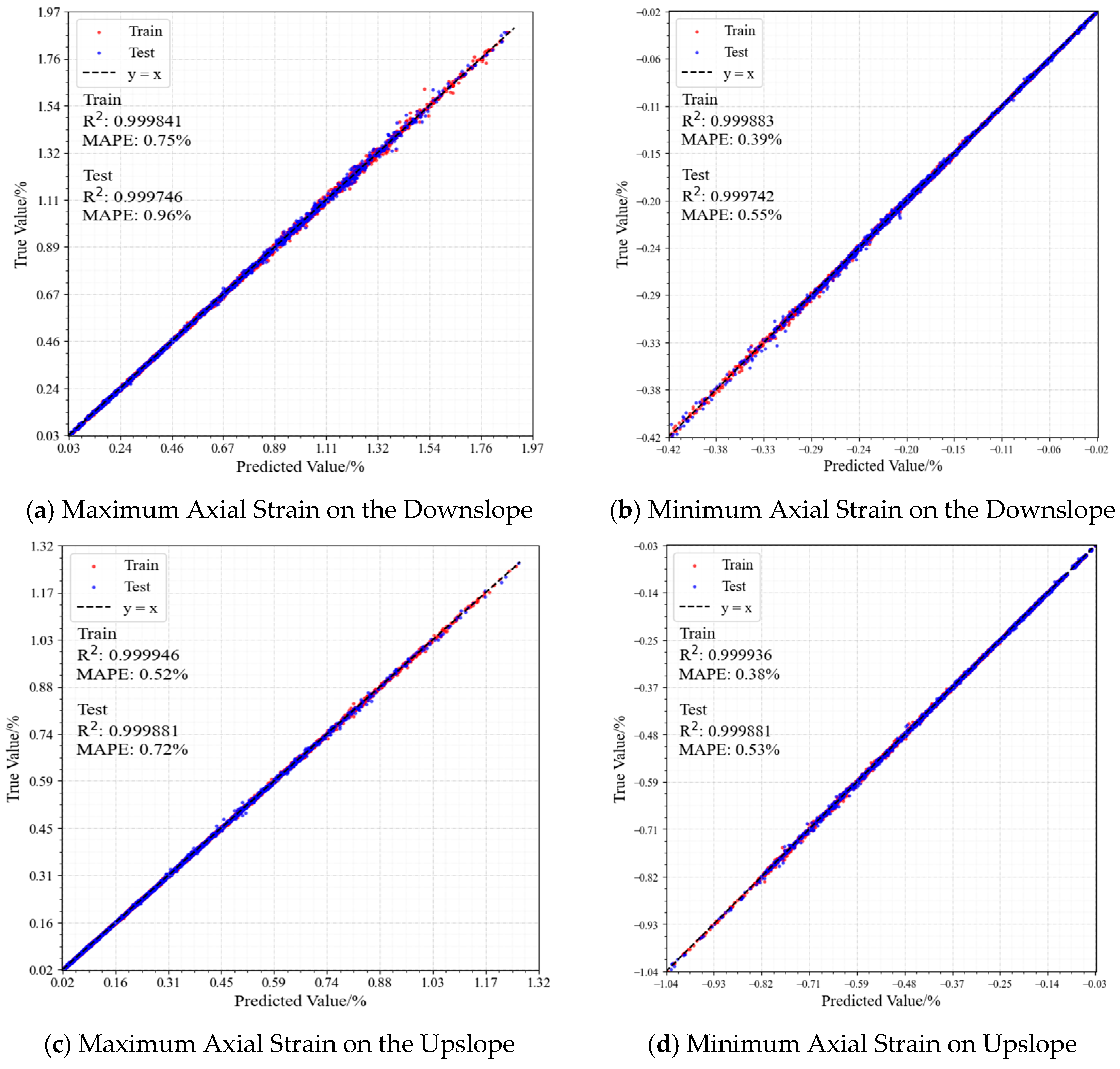
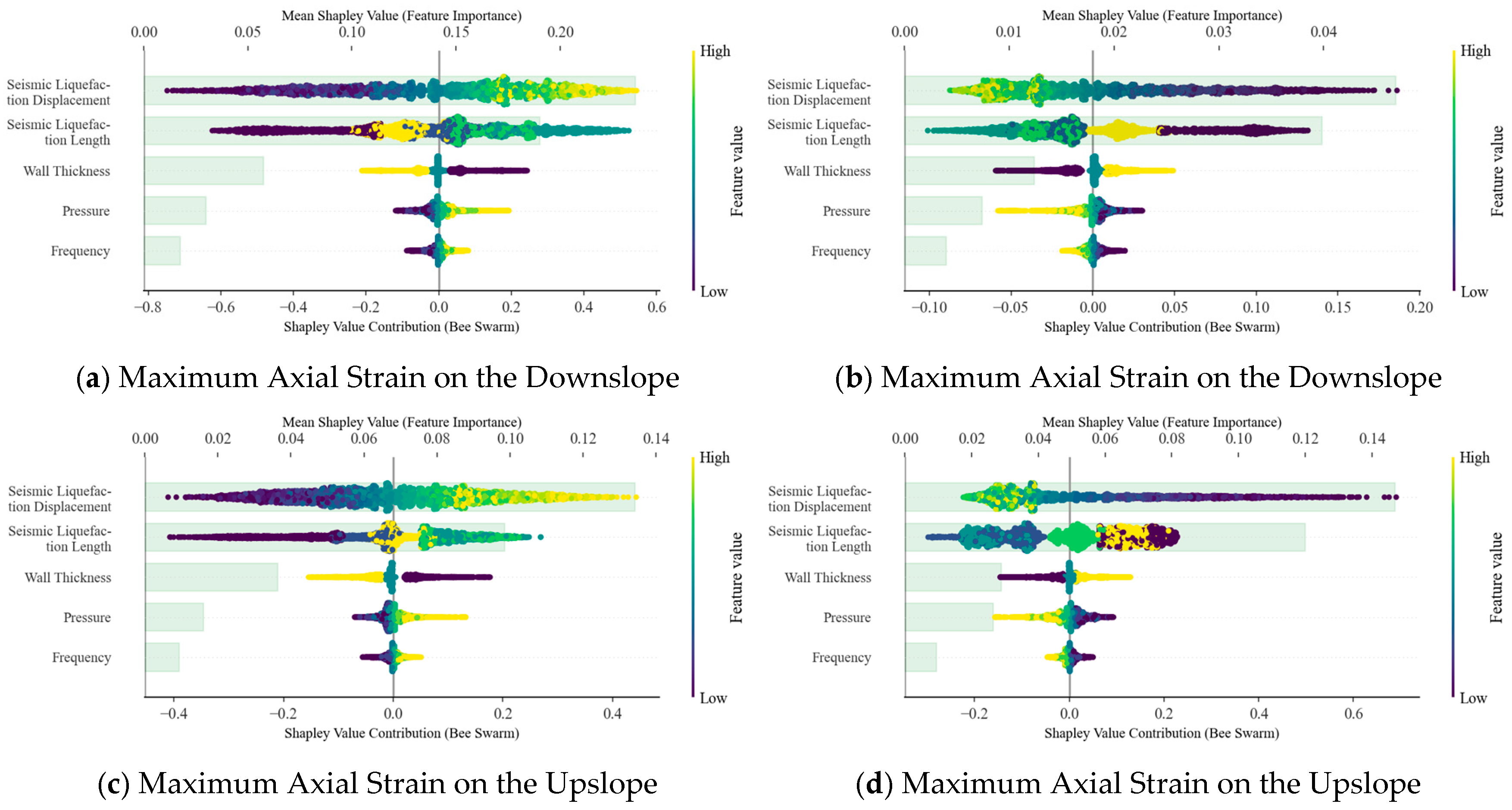
The validated optimal prediction model for pipeline safety under seismic liquefaction-induced displacement demonstrates outstanding performance in predicting axial strain peaks, with R² and MAPE values of 0.99975 and 0.96071% for passive side maximum axial strain, 0.99974 and 0.54622% for passive side minimum axial strain, 0.99988 and 0.71701% for active side maximum axial strain, and 0.99988 and 0.53409% for active side minimum axial strain, respectively. These results confirm the model’s high accuracy in predicting pipeline strain extremes caused by liquefaction displacement. SHAP-based interpretability analysis is also performed on the developed model. The results indicate that liquefaction-induced displacement is the most critical factor affecting the maximum and minimum axial strains on both the upslope and downslope sides of the pipeline under seismic liquefaction. Additionally, increasing the pipeline wall thickness can effectively mitigate deformation caused by liquefaction.

(4)

The model’s performance is contingent on the validity of the underlying FEM simulations and experimental data, primarily applicable to clayey soils and the specific displacement pattern used. Generalization to sandy liquefiable soils, complex 3D ground motion, or different pipeline configurations requires further validation.

(5)

Future research should focus on: (a) validating the model against field case studies or centrifuge test data, (b) extending the approach to sandy liquefiable soils, (c) incorporating spatial variability of ground motion and soil properties, and (d) exploring the integration of real-time sensor data for online model updating and prognostics.

References

1. EI Hmadi, K.; O’Rourke, M.J. Soil Springs for Buried Pipeline Axial Motion. J. Geotech. Eng. ASCE 1988, 114, 1335–1339. [Google Scholar] [CrossRef]
2. Guo, E.D.; Feng, Q.M. Aseismic Analysis Method for Buried Steel Pipe Crossing Fault. Earthq. Eng. Eng. Vib. 1999, 19, 43–47. [Google Scholar]
3. Feng, Q.M.; Guo, E.D. Seismic Performance Testing of Pipeline Structures Crossing Active Faults. Earthq. Eng. Eng. Vib. 2000, 20, 56–63. [Google Scholar]
4. Hindy, A.; Novak, M. Earthquake response of under ground pipeline. Int. J. Earthq. Eng. Struct. Dyn. 1979, 7, 451–476. [Google Scholar] [CrossRef]
5. Xu, J.C.; Jian, W.B.; Shang, Y.Q. Study on the Seismic Failure Mechanism of the Thick Soft Soil Foundation. Chin. J. Rock Mech. Eng. 2005, 24, 313–320. [Google Scholar]
6. Madabhushi, S.; Madabhushi, S. Finite Element Analysis of Floatation of Rectangular Tunnels Following Earthquake Induced Liquefaction. Indian Geotech. J. 2014, 45, 233–242. [Google Scholar] [CrossRef]
7. Azadi, M.; Hosseini, S.M.M.M. The uplifting behavior of shallow tunnels within the liquefiable soils under cyclic loading. Tunn. Undergr. Space Technol. 2010, 25, 158–167. [Google Scholar] [CrossRef]
8. Tang, A.P.; Li, Z.Q.; Feng, R.C.; Zhou, X.Y. Model Experiment and Analysis on Seismic Response of Utility Tunnel Systems Using a Shaking Table. Chin. J. Rock Mech. Eng. 2009, 41, 1–5. [Google Scholar]
9. American Lifelines Alliance—American Society of Civil Engineers. Guidelines for the Design of Buried Steel Pipe (with Addenda through February 2005). 2001. Available online: https://www.americanlifelinesalliance.com/pdf/Update061305.pdf (accessed on 1 May 2025).
10. Saeedzadeh, R.; Hataf, N. Uplift response of buried pipelines in saturated sand deposit under earthquake loading. Soil Dyn. Earthq. Eng. 2011, 31, 1378–1384. [Google Scholar] [CrossRef]
11. Yan, K.; Zhang, J.; Wang, Z.; Liao, W.; Wu, Z. Seismic responses of deep buried pipeline under non-uniform excitations from large scale shaking table test. Soil Dyn. Earthq. Eng. 2018, 113, 180–192. [Google Scholar] [CrossRef]
12. ABAQUS. ABAQUS User’s Manual, version 6.11.; Simulia: Providence, RI, USA, 2011. [Google Scholar]
13. GB50470-2017; Seismic Technical Code for Oil and Gas Transmission Pipeline Engineering. China Planning Press: Beijing, China, 2017.
14. O’Rourke, M.J.; Liu, X. Seismic Design of Buried and Offshore Pipelines; MCEER-12-MN04; University at Buffalo, State University of New York: Buffalo, NY, USA, 2012; p. 158. [Google Scholar]
15. Feurer, M.; Eggensperger, K.; Falkner, S.; Lindauer, M.; Hutter, F. Auto-sklearn 2.0: Hands-free automl via meta-learning. J. Mach. Learn. Res. 2022, 23, 1–61. [Google Scholar]
16. Feurer, M.; Klein, A.; Eggensperger, K.; Springenberg, J.; Blum, M.; Hutter, F. Efficient and robust automated machine learning. Adv. Neural Inf. Process. Syst. 2015, 28. [Google Scholar]
17. Wang., C.; Wu, Q.; Weimer, M.; Zhu, E. FLAML: A Fast and Lightweight AutoML Library. Proc. Mach. Learn. Syst. 2021, 3, 434–447. [Google Scholar]
18. Ke, G.; Meng, Q.; Finley, T.; Wang, T.; Chen, W.; Ma, W.; Ye, Q.; Liu, T.-Y. Lightgbm: A highly efficient gradient boosting decision tree. Adv. Neural Inf. Process. Syst. 2017, 30. [Google Scholar]
19. Shakeel, A.; Chong, D.; Wang, J. District heating load forecasting with a hybrid model based on LightGBM and FB-prophet. J. Clean. Prod. 2023, 409, 137130. [Google Scholar] [CrossRef]
20. Chen, T.; Guestrin, C. Xgboost: A Scalable Tree Boosting System. In Proceedings of the 22nd ACM SIGKDD International Conference on Knowledge Discovery and Data Mining, San Francisco, CA, USA, 13–17 August 2016; pp. 785–794. [Google Scholar]
21. Zhou, S. Gwo-ga-xgboost-based model for Radio-Frequency power amplifier under different temperatures. Expert Syst. Appl. 2025, 278, 127439. [Google Scholar] [CrossRef]
22. Prokhorenkova, L.; Gusev, G.; Vorobev, A.; Dorogush, A.V.; Gulin, A. CatBoost: Unbiased boosting with categorical features. Adv. Neural Inf. Process. Syst. 2018, 31. [Google Scholar]
23. Fan, Z.; Gou, J.; Weng, S. Complementary CatBoost based on residual error for student performance prediction. Pattern Recognit. 2025, 161, 111265. [Google Scholar] [CrossRef]
24. Peng, H.; Lu, H.; Xu, Z.-D.; Wang, Y.; Zhang, Z. Predicting Solid-Particle Erosion Rate of Pipelines Using Support Vector Machine with Improved Sparrow Search Algorithm. J. Pipeline Syst. Eng. Pract. 2023, 14, 04022077. [Google Scholar] [CrossRef]
25. Lu, H.; Iseley, T.; Matthews, J.; Liao, W. Hybrid machine learning for pullback force forecasting during horizontal directional drilling. Autom. Constr. 2021, 129, 103810. [Google Scholar] [CrossRef]
26. Lundberg, S.M.; Lee, S.I. A unified approach to interpreting model predictions. Adv. Neural Inf. Process. Syst. 2017, 30. [Google Scholar]
Figure 1. Workflow of the proposed method.
Processes 13 02163 g001
Figure 2. Layout of external pipeline strain gauges and soil pressure transducers.
Processes 13 02163 g002
Figure 3. Assembled model inside the test container.
Processes 13 02163 g003
Figure 4. Dynamic loading conditions.
Processes 13 02163 g004
Figure 5. Displacement–soil pressure curves at monitoring points under horizontal seismic excitation with different frequency loads.
Processes 13 02163 g005
Figure 6. Modified soil spring model.
Processes 13 02163 g006
Figure 7. Fitted amplification factor curves under horizontal dynamic loading.
Processes 13 02163 g007
Figure 8. Finite element model of pipe–soil interaction.
Processes 13 02163 g008
Figure 9. True stress–strain curve of X80 steel.
Processes 13 02163 g009
Figure 10. Schematic diagram of lateral soil liquefaction displacement.
Processes 13 02163 g010
Figure 11. Comparison of pipeline axial strain under different liquefaction zone lengths.
Processes 13 02163 g011
Figure 12. Comparison of maximum axial strain in pipelines with different liquefaction zone lengths.
Processes 13 02163 g012
Figure 13. Comparison of pipeline axial strain under different seismic wave frequencies.
Processes 13 02163 g013
Figure 14. Comparison of maximum axial strain in pipelines under different seismic wave frequencies.
Processes 13 02163 g014
Figure 15. Comparison of pipeline axial strain under different internal pressures.
Processes 13 02163 g015
Figure 16. Comparison of maximum axial strain in pipelines under different internal pressures.
Processes 13 02163 g016
Figure 17. Comparison of pipeline axial strain under different wall thicknesses.
Processes 13 02163 g017
Figure 18. Comparison of maximum axial strain in pipelines under different wall thicknesses.
Processes 13 02163 g018
Figure 19. Auto machine learning computational flow.
Processes 13 02163 g019
Figure 20. Automation flowchart for the construction of intelligent prediction model for pipeline structural safety state under seismic liquefaction displacement.
Processes 13 02163 g020
Figure 21. Optimal prediction model for pipeline safety state under seismic liquefaction.
Processes 13 02163 g021
Figure 22. SHAP model interpretation for pipeline safety state under seismic liquefaction.
Processes 13 02163 g022