
Influence of Operating Conditions on the Energy Consumption of CO2 Supermarket Refrigeration Systems


Abstract
1. Introduction
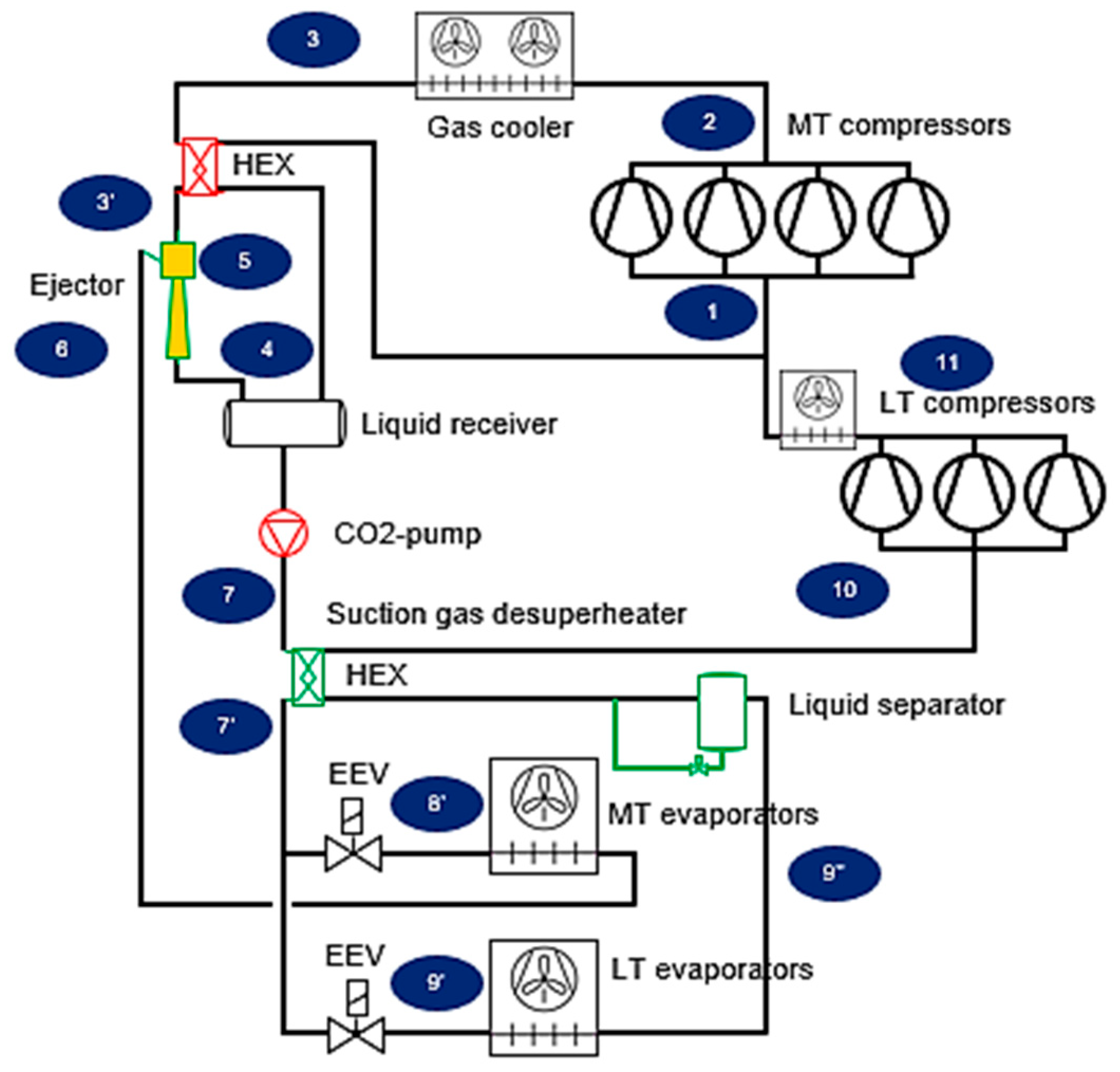
2. Materials and Methods
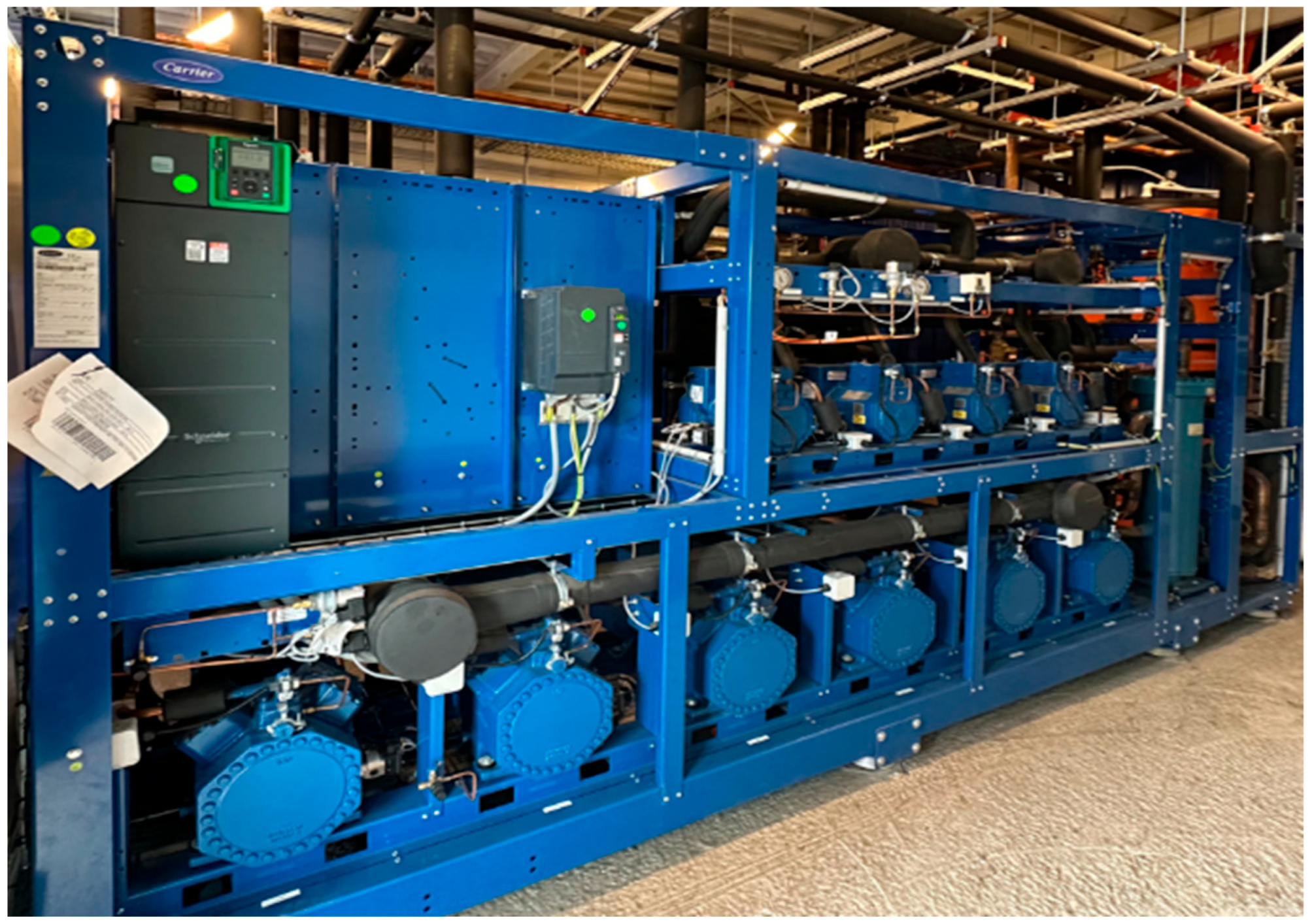
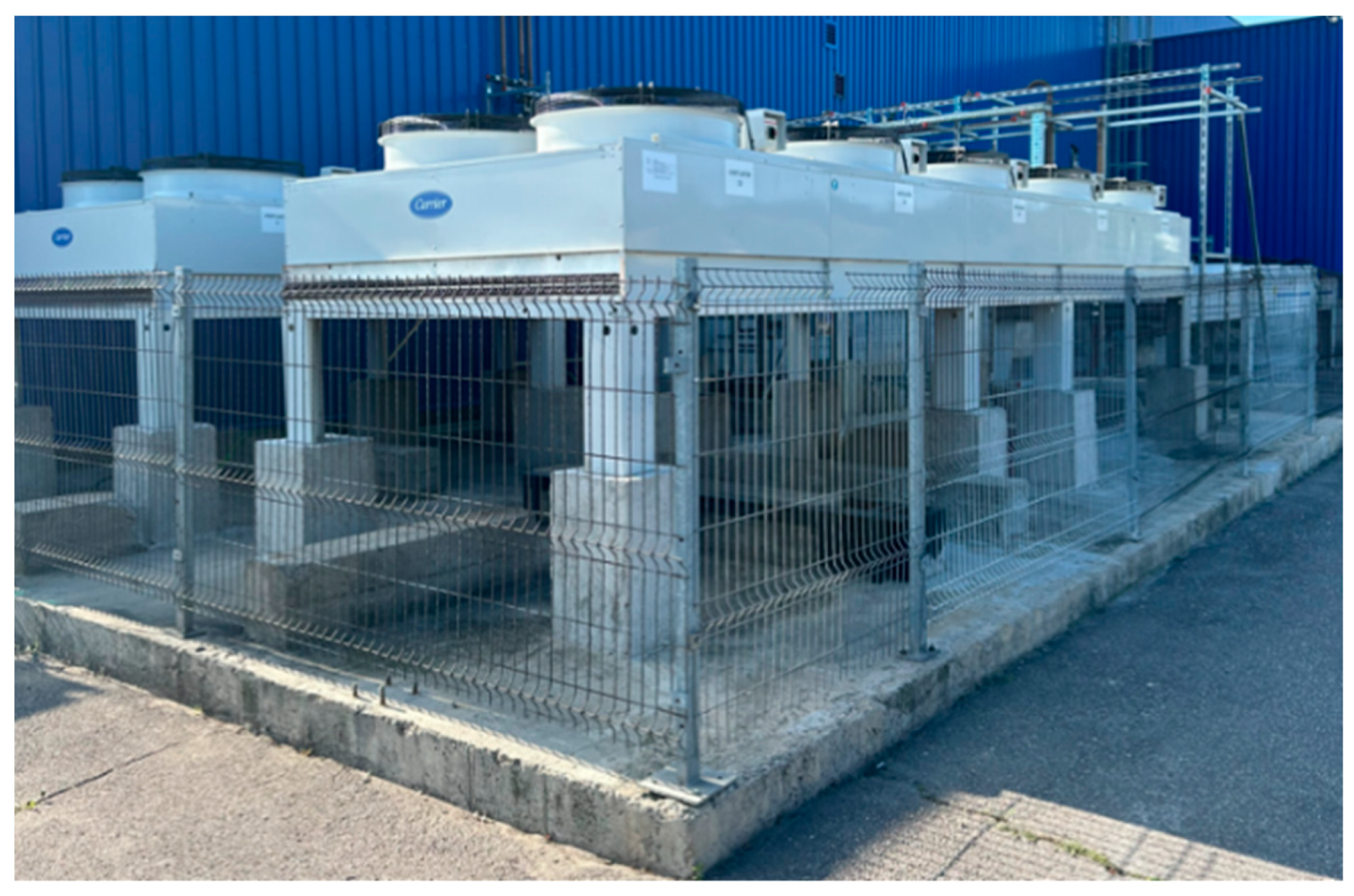
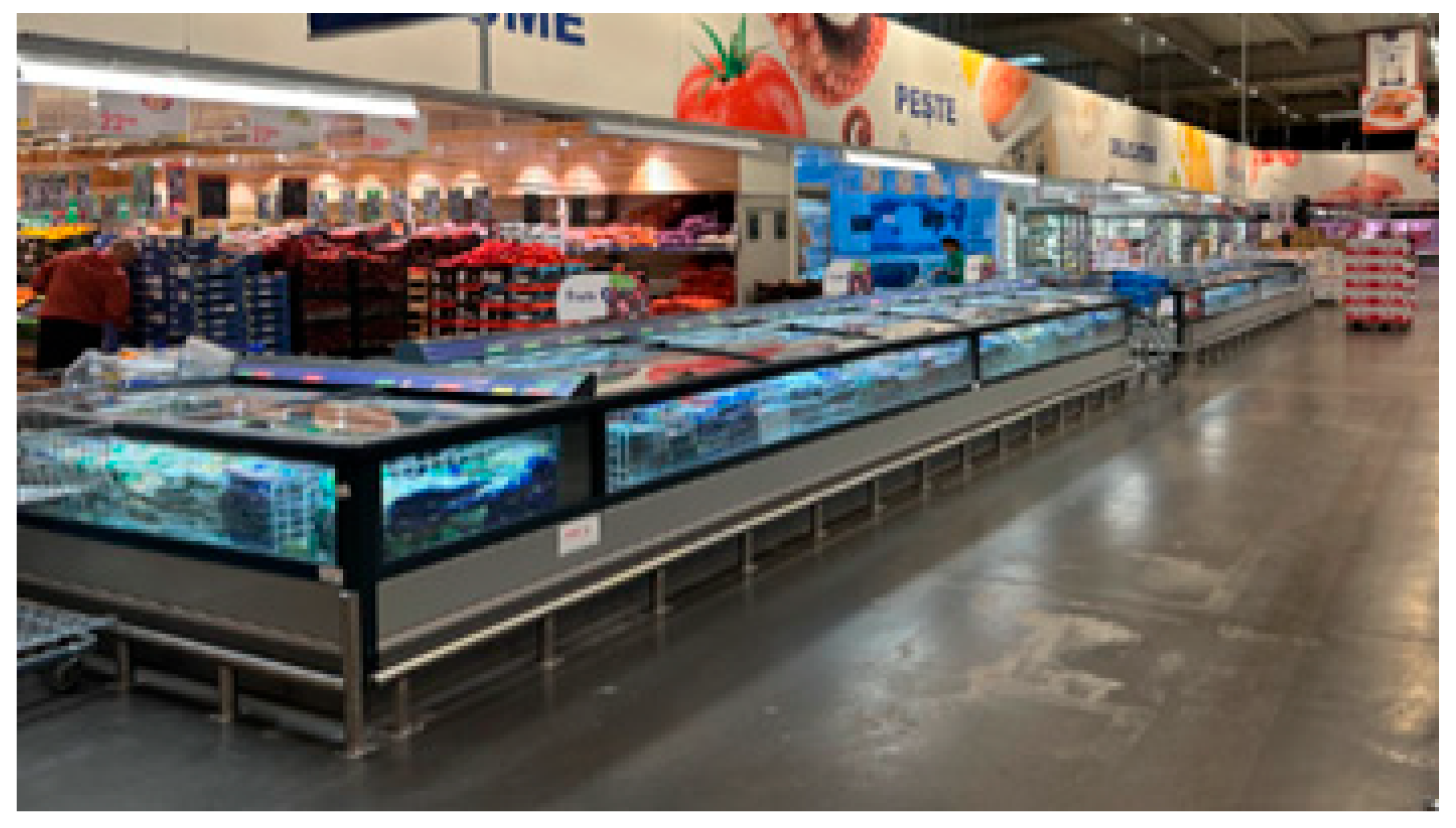
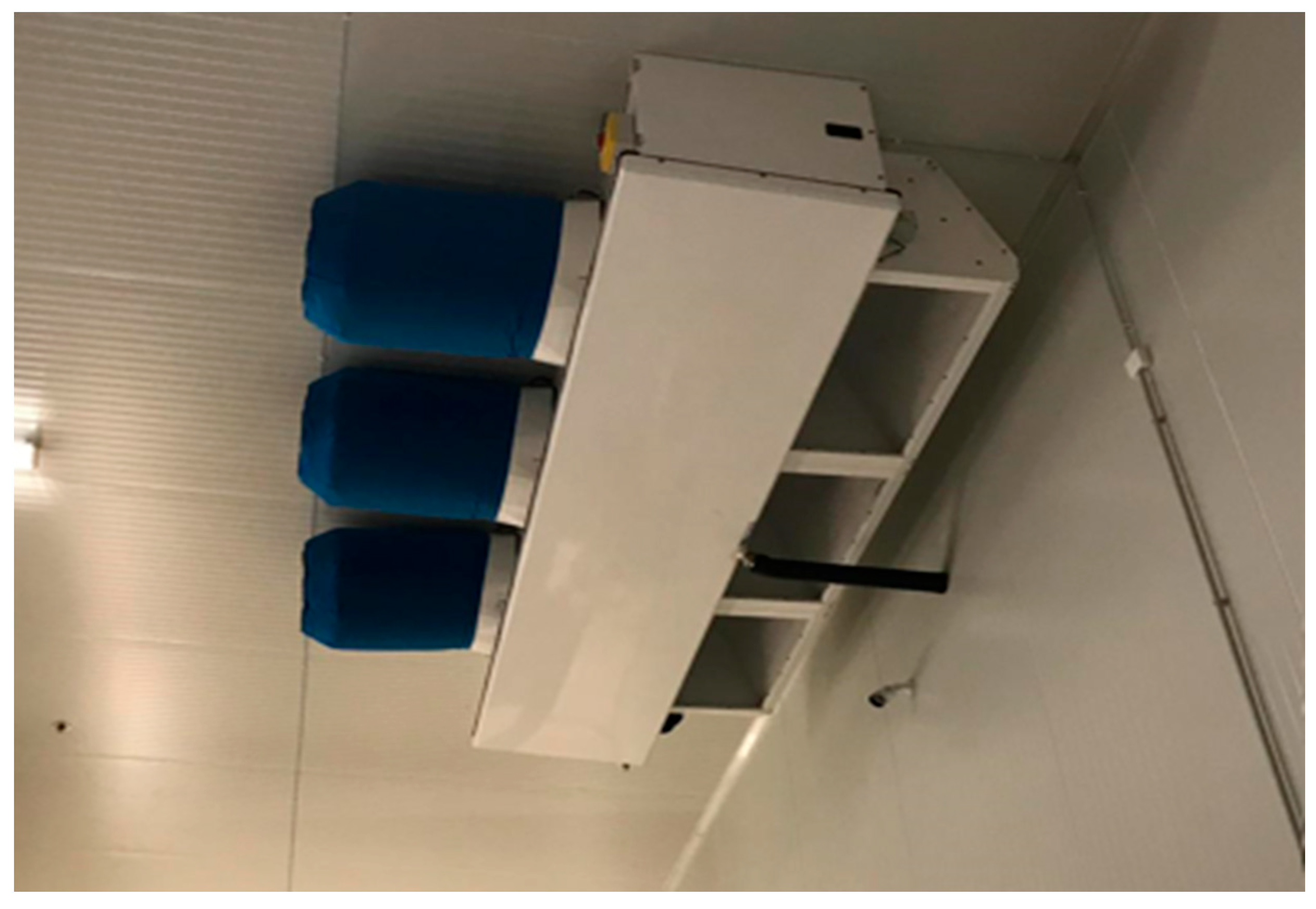
Description of the Studied Systems
- Sensors for measuring consumer temperature (display cabinets and cold rooms are of the NTC type, which can operate in the temperature range of −50 °C to +50 °C).
- Sensors for measuring the temperature of compressor racks and gas coolers, PT1000 type, which can operate in the temperature range of −50 °C to +200 °C.
- Sensors for suction-pressure measurement: 4–20 mA; 1–26 bar.
- Sensors for medium-pressure measurement: 4–20 mA; 1–59 bar.
- Sensors for high-pressure measurement: 4–20 mA; 1–161 bar.
- Schneider energy consumption recorders of type iEM3255 with an accuracy of ±1 A.
3. Energy Model
3.1. Compressors
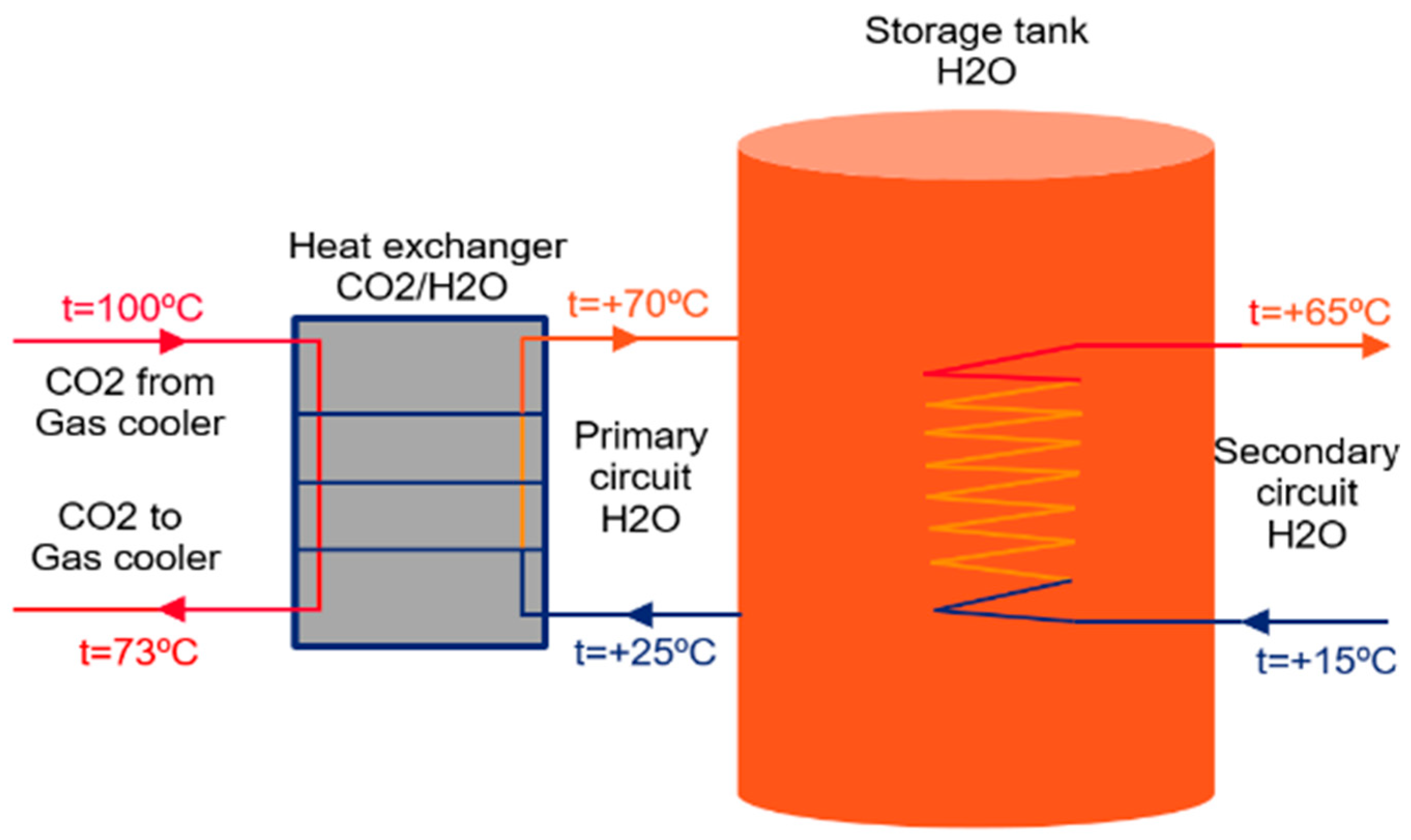
3.2. Gas Cooler
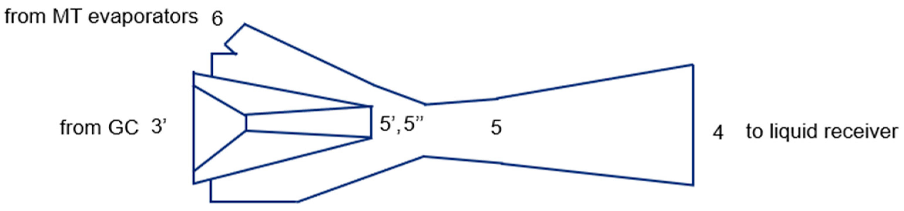
3.3. Ejector
- −
- If the liquid receiver pressure Pr is not higher than the critical pressure Prc, and the ejector is working at critical mode, then
- −
- If Pr is between the critical pressure Prc and the breakdown pressure Prb, the entrainment ratio u can be obtained by the following equation:
3.4. Electronic Expansion Valves
3.5. Evaporators in Cold Rooms and Display Cabinets
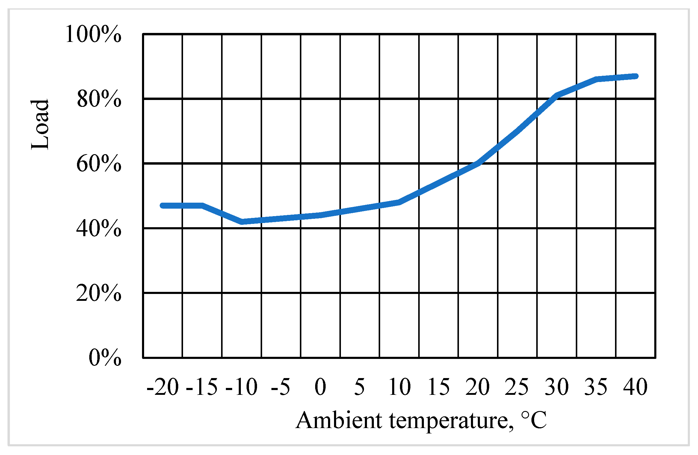
4. Estimation of Annual Energy Consumption
- −
- All thermodynamic transformations occur in steady-state;
- −
- Pressure drops in heat exchangers are neglected;
- −
- Expansion processes in the expansion valves are assumed to be isenthalpic;
- −
- Efficiency of liquid–vapour separation in liquid receiver is 100%;
- −
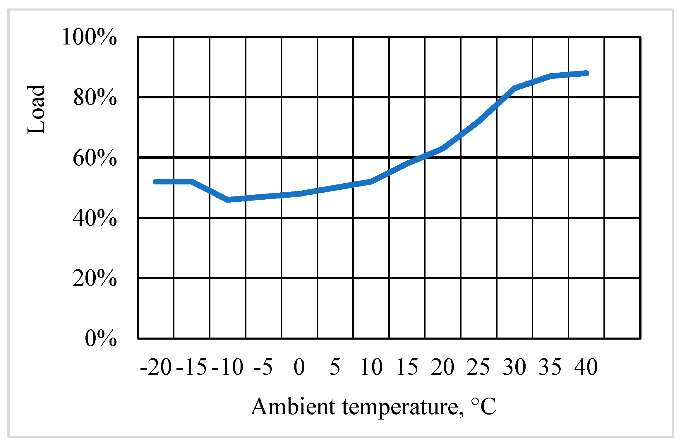
- The outside temperature varies from −20 °C to +40 °C.
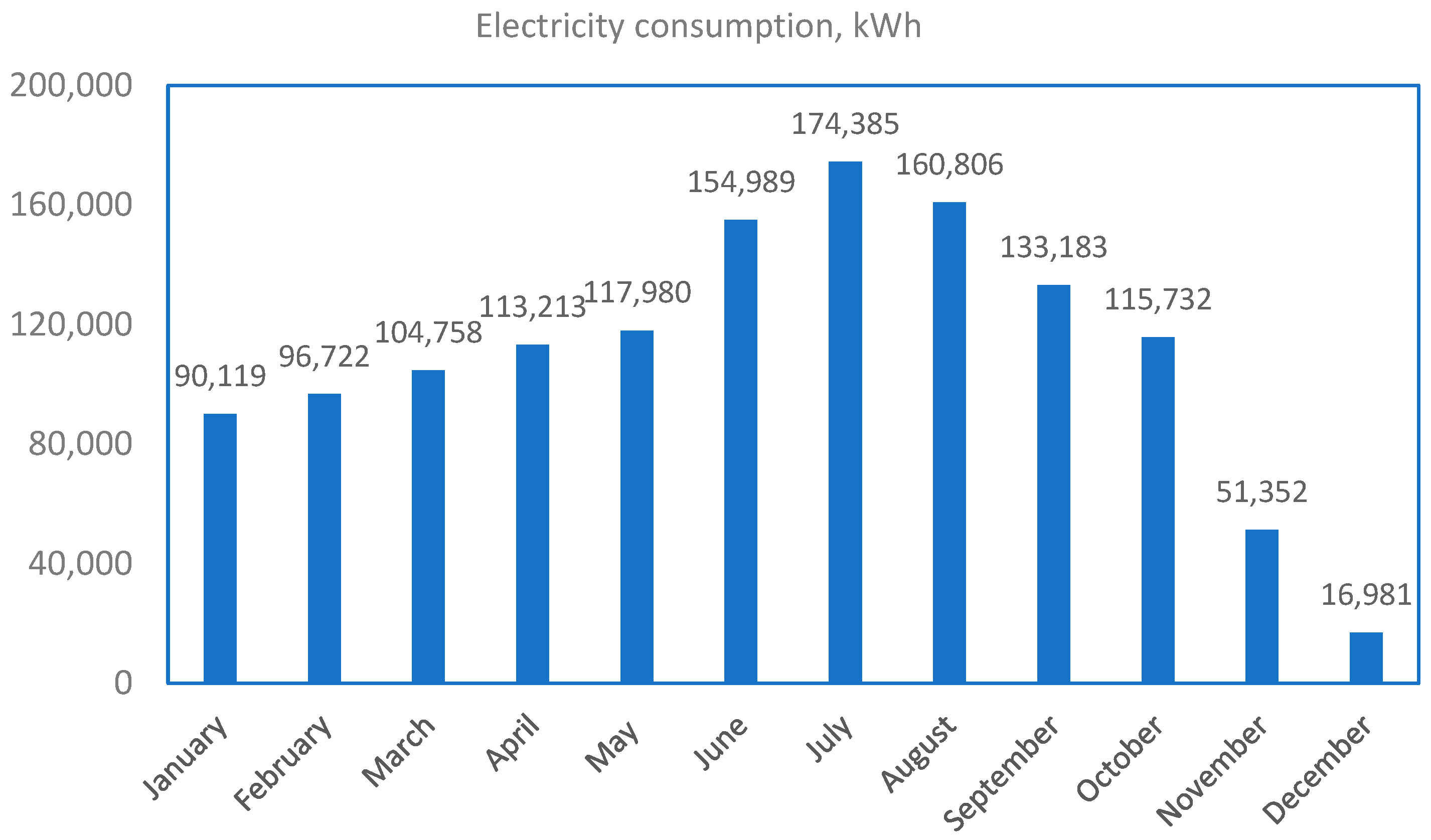
5. Results and Discussion
6. Conclusions
Author Contributions
Funding
Data Availability Statement
Acknowledgments
Conflicts of Interest
Nomenclature
| Abbreviations | |
| ah | Air absolute humidity in kg/kg |
| C1, C2, C3, C4, C5 | Constants |
| cp | Specific heat at constant pressure in kJ/kg·K |
| cv | Specific heat at constant volume in kJ/kg·K |
| CO2 | Carbon dioxide |
| COP | Coefficient of performance |
| CS | Cascade system |
| EEV | Electronic expansion valve |
| EJ | Ejector |
| EOM | Equation-oriented method |
| GC | Gas cooler |
| GWP | Global warming potential |
| HER | Heat extraction rate |
| HEX | Heat exchanger |
| HFC | Hydrofluorocarbon |
| HP | High pressure |
| HR | Heat recovery |
| HVAC&R | Heating, ventilation, air conditioning, and refrigeration |
| LP | Low pressure |
| LS | Liquid separator |
| LT | Low temperature |
| Mass flow rate in kg·s−1 | |
| MEJ | Multi-ejector |
| MP | Medium pressure |
| MT | Medium temperature |
| Natref | Natural refrigerant |
| ODS | Ozone depleting substance |
| OilP | Oil pressure |
| p | Pressure in Pa |
| PC | Parallel compression |
| R | Gas constant in J·kg−1·K−1 |
| RDC | Refrigerated display cabinet |
| RH | Air relative humidity in % |
| S | Surface in m2 |
| SAM | Successive approximation method |
| SCM | Sequential component method |
| Synrefs | Synthetic refrigerant |
| T | Temperature in K |
| TEWI | Total Equivalent Warming Impact |
| u | Entrainment ratio |
| V | Volume in m3 |
| V | Velocity in m·s−1 |
| W | Electrical power in kW |
| ε | GC efficiency |
| Φ | Heat flow rate in kW |
| Γ | Isentropic exponent |
| λ | Coefficient of friction |
| η | Isentropic efficiency |
| γ | Adiabatic exponent |
| ρ | Density in kg/m3 |
| Subscripts | |
| ai | Air inlet |
| ao | Air outlet |
| comp | Compression |
| d | Discharge |
| p | Primary |
| r | Refrigerant |
| ri | Refrigerant inlet |
| ro | Refrigerant outlet |
| s | Suction; secondary |
| sat | Saturated |
| sh | Superheated |
| tp | Two-phase |
| V | Volumetric |
| ve | Expansion valve |
| w | Condensate |
| m | Logarithmic mean |
| mf | Missing flow |
| max | Maximum |
| min | Minimum |
| rc | To receiver, critical |
| s | Secondary flow |
| y | Position of the hypothetical throat |
| u | Critical entrainment ratio |
References
- Dilshad, S.; Kalair, A.R.; Khan, N. Review of carbon dioxide (CO2) based heating and cooling technologies: Past, present, and future outlook. Int. J. Energy Res. 2020, 44, 1408–1463. [Google Scholar] [CrossRef]
- Sawalha, S.; Piscopiello, S.; Karampour, M.; Manickam, L.; Rogstam, J. Field measurements of supermarket refrigeration systems. Part II: Analysis of HFC refrigeration systems and comparison to CO2 trans-critical. Appl. Therm. Eng. 2017, 111, 170–182. [Google Scholar] [CrossRef]
- Liao, S.M.; Zhao, T.S.; Jakobsen, A. Correlation of optimal heat rejection pressures in transcritical carbon dioxide cycles. Appl. Therm. Eng. 2000, 20, 831–841. [Google Scholar] [CrossRef]
- Vidan-Falomir, F.; Larrondo-Sancho, R.; Sanchez, D.; Cabello, R. Evaluation of different subcooling arrangements in a CO2 refrigeration plant using extractions from the flash-gas tank. Int. J. Refrig. 2025, 175, 334–344. [Google Scholar] [CrossRef]
- Ge, Y.T.; Tassou, S.A. Thermodynamic analysis of transcritical CO2 booster refrigeration systems in supermarket. Energy Convers. Manag. 2011, 52, 1868–1875. [Google Scholar] [CrossRef]
- Dubey, A.M.; Kumar, S.; Agrawal, G.D. Thermodynamic analysis of a transcritical CO2/propylene (R744–R1270) cascade system for cooling and heating applications. Energy Convers. Manag. 2014, 86, 774–783. [Google Scholar] [CrossRef]
- Llopis, R.; Cabello, R.; Sánchez, D.; Torrella, E. Energy improvements of CO2 transcritical refrigeration cycles using dedicated mechanical subcooling. Int. J. Refrig. 2015, 55, 129–141. [Google Scholar] [CrossRef]
- Śmierciew, K.; Butrymowicz, D.; Gagan, J.; Jakończuk, P.; Pawłowski, M. Design and Manufacture of a Micro-Ejector and the Testing Stand for Investigation of Micro-Ejector Refrigeration Systems. Micromachines 2024, 15, 429. [Google Scholar] [CrossRef]
- Pardiñas, Á.Á.; Hafner, A.; Banasiak, K. Novel integrated CO2 vapour compression racks for supermarkets. Thermodynamic analysis of possible system configurations and influence of operational conditions. Appl. Therm. Eng. 2018, 131, 1008–1025. [Google Scholar] [CrossRef]
- Sengupta, A.; Gullo, P.; Dasgupta, M.S.; Khorshidi, V. Performance Analysis of an R744 Supermarket Refrigeration System Integrated with an Organic Rankine Cycle. Energies 2023, 16, 7478. [Google Scholar] [CrossRef]
- Sarkar, J.; Agrawal, N. Performance optimization of transcritical CO2 cycle with parallel compression economization. Int. J. Therm. Sci. 2010, 49, 838–843. [Google Scholar] [CrossRef]
- Gullo, P.; Hafner, A.; Cortella, G. Multi-ejector R744 booster refrigerating plant and air conditioning system integration—A theoretical evaluation of energy benefits for supermarket applications. Int. J. Refrig. 2017, 75, 164–176. [Google Scholar] [CrossRef]
- Karampour, M.; Sawalha, S. State-of-the-art integrated CO2 refrigeration system for supermarkets: A comparative analysis. Int. J. Refrig. 2018, 86, 239–257. [Google Scholar] [CrossRef]
- Polzot, A.; D’Agaro, P.; Cortella, G. Energy analysis of a transcritical CO2 supermarket refrigeration system with heat recovery. Energy Procedia 2017, 111, 648–657. [Google Scholar] [CrossRef]
- Steuer, D.; Termens, J.; Arias, J.; Sawalha, S. Thermal energy export from supermarket refrigeration systems: Drivers and barriers. Energy Rep. 2024, 12, 5875–5885. [Google Scholar] [CrossRef]
- Evans, J.; Hammond, E.; Gigiel, A.; Reinholdt, L.; Fikiin, K.; Zilio, C. Improving the energy performance of cold stores. In Proceedings of the 2nd IIR Conference on Sustainability and the Cold Chain, Paris, France, 2–4 April 2013; International Institute of Refrigeration: Paris, France. Available online: https://iifiir.org/en/fridoc/improving-the-energy-performance-of-cold-stores-29339 (accessed on 13 December 2024).
- Evans, J.A.; Hammond, E.C.; Gigiel, A.J.; Fostera, A.M..; Reinholdt, L.; Fikiin, K.; Zilio, C. Assessment of methods to reduce the energy consumption of food cold stores. Appl. Therm. Eng. 2014, 62, 697–705. [Google Scholar] [CrossRef]
- Evans, J.A.; Foster, A.M.; Huet, J.M.; Reinholdt, L.; Fikiin, K.; Zilio, C.; Houska, M.; Landfeld, A.; Bond, C.; Scheurs, M.; et al. Specific energy consumption values for various refrigerated food cold stores. Energy Build. 2014, 74, 141–151. [Google Scholar] [CrossRef]
- ISO 23953-1:2024; Refrigerated display cabinets—Part 1: Vocabulary. International Organization for Standardization (ISO): Geneva, Switzerland, 2024.
- Mousset, S.; Libsig, M. Energy Consumptions of Display Cabinets in Supermarket. 2011. Available online: https://iifiir.org/en/fridoc/energy-consumptions-of-display-cabinets-in-a-supermarket-28145 (accessed on 13 December 2024).
- Bahman, A.; Rosario, L.; Rahman, M.M. Analysis of energy savings in a supermarket refrigeration/HVAC system. Appl. Energy 2012, 98, 11–21. [Google Scholar] [CrossRef]
- Ge, Y.T.; Tassou, S.A. Control optimizations for heat recovery from CO2 refrigeration systems in supermarket. Energy Convers. Manag. 2014, 78, 245–252. [Google Scholar] [CrossRef]
- Constantino, M.C.; Kanizawa, F.T. Evaluation of pressure drop effect on COP of single-stage vapor compression refrigeration cycles. Therm. Sci. Eng. Prog. 2022, 28, 101048. [Google Scholar] [CrossRef]
- Oldřich, J. Isentropic efficiency of centrifugal compressor working with real gas. Acta Polytech. CTU Proc. 2018, 20, 65–72. [Google Scholar] [CrossRef]
- Li, D.; Groll, E.A. Transcritical CO2 refrigeration cycle with ejector-expansion device. Int. J. Refrig. 2005, 28, 766–773. [Google Scholar] [CrossRef]
- Lei, Y.; Li, S.; Lu, J.; Xu, Y.; Yong, Y.; Xing, D. Numerical Analysis of Steam Ejector Performance with Non-Equilibrium Condensation for Refrigeration Applications. Buildings 2023, 13, 1672. [Google Scholar] [CrossRef]
- Bankole, A.T.; Bello-Salau, H.; Haruna, Z. Nonlinear Identification of the Suction Manifold of a Supermarket Refrigeration System Using Wavelet Networks. Eng. Proc. 2024, 67, 37. [Google Scholar] [CrossRef]
- Bitzer Websoftware. Available online: https://www.bitzer.de/websoftware/calculate/HHK/?tab=results (accessed on 22 February 2025).
- Sun, J.; Kuruganti, T.; Munk, J.; Dong, J.; Cui, B. Low global warming potential (GWP) refrigerant supermarket refrigeration system modeling and its application. Int. J. Refrig. 2021, 126, 195–209. [Google Scholar] [CrossRef]
- Kim, M.H.; Bullard, C.W. Thermal performance analysis of small hermetic refrigeration and air-conditioning compressor. JEME Int. J. Ser. B. 2002, 45, 857–864. [Google Scholar] [CrossRef]
- Sun, J.; Li, W. Operation optimization of an Organic Rankine cycle (ORC) heat recovery power plant. Appl. Therm. Eng. 2011, 31, 2032–2041. [Google Scholar] [CrossRef]
- Sawalha, S.; Karampour, M.; Rogstam, J. Field measurements of supermarket refrigeration systems. Part I: Analysis of CO2 transcritical refrigeration systems. Appl. Therm. Eng. 2015, 87, 633–647. [Google Scholar] [CrossRef]
- Li, F.; Tian, Q.; Wu, C.; Wang, X.; Lee, J.M. Ejector performance prediction at critical and subcritical operational modes. Appl. Therm. Eng. 2017, 115, 444–454. [Google Scholar] [CrossRef]
- Sun, J.; Reddy, A.T. A new approach to develop building energy system simulation programs suitable for both design and optimal operation. ASHRAE Trans. 2006, 112, 729–738. [Google Scholar]
- Xue, X.; Feng, X.; Wang, J.; Liu, F. Modeling and Simulation of an Air-cooling Condenser under Transient Conditions. Procedia Eng. 2012, 31, 817–822. [Google Scholar] [CrossRef]
- Bendaoud, A.; Ouzzane, M.; Aidoun, Z.; Galanis, N. A new modeling approach for the study of finned coils with CO2. Int. J. Therm. Sci. 2010, 49, 1702–1711. [Google Scholar] [CrossRef]
- Kuehn, T.; Ramsey, J.W.; Threlkeld, J.L. Thermal Environmental Engineering, 3rd ed.; Prentice-Hall: Upper Saddle River, NJ, USA, 1998; pp. 314–445. [Google Scholar]
- Lemmon, E.W.; Huber, M.L.; McLinden, M.O. Reference Fluid Thermodynamic and Transport Properties-REFPROP, Version 9.1; National Institute of Standards and Technology: Gaithersburg, MD, USA, 2013; Standard Reference Data Program. Available online: https://www.nist.gov/publications/nist-standard-reference-database-23-reference-fluid-thermodynamic-and-transport (accessed on 15 December 2024).
- Söylemez, E. Energy and Conventional Exergy Analysis of an Integrated Transcritical CO2 (R-744) Refrigeration System. Energies 2024, 17, 479. [Google Scholar] [CrossRef]


| Parameter | Value |
|---|---|
| Useful superheat—LT | ΔtusLT = 6 K |
| Useful superheat—MT | ΔtusMT = 6 K |
| Suction line superheat—LT | ΔtsLT = 14 K |
| Suction line superheat—MT | ΔtsMT = 9 K |
| Maximum frequency of 1st compressor | 70 Hz |
| Minimum frequency of 1st compressor | 30 Hz |
| Pump efficiency refrigerant pump | 10% |
| Minimum condensing temperature—LT | 5 °C |
| Subcooling | 0.5 °C |
| Maximum high pressure | 98 bar |
| Temp. difference for desuperheater | Δt = 5 K |
| Defrost timing—MT | 2 h/day |
| Defrost timing—LT | 1.5 h/day |
| Outdoor Temperature, °C | Operating Hours, h | Adiabatic Inlet Temperature, °C |
|---|---|---|
| +40 | 0 | +32.4 |
| +35 | 94 | +27.4 |
| +30 | 512 | +29.9 |
| +25 | 1008 | +25 |
| +20 | 1414 | +20 |
| +15 | 1501 | +15 |
| +10 | 1375 | +10 |
| +5 | 1433 | +5 |
| 0 | 931 | 0 |
| −5 | 303 | −5 |
| −10 | 154 | −10 |
| −15 | 35 | −15 |
| −20 | 0 | −20 |
| Freezing Circuit | Value |
|---|---|
| t0 freezing—consumers | −29.0 °C |
| Δt according to Δp piping network | +1.5 K |
| t0 freezing—compressors | −30.5 °C |
| Refrigeration Circuit | Value |
| t0 refrigeration—consumers | −3.0 °C |
| Δt according Δp piping network | +2.0 K |
| t0 refrigeration—compressors | −5.0 °C |
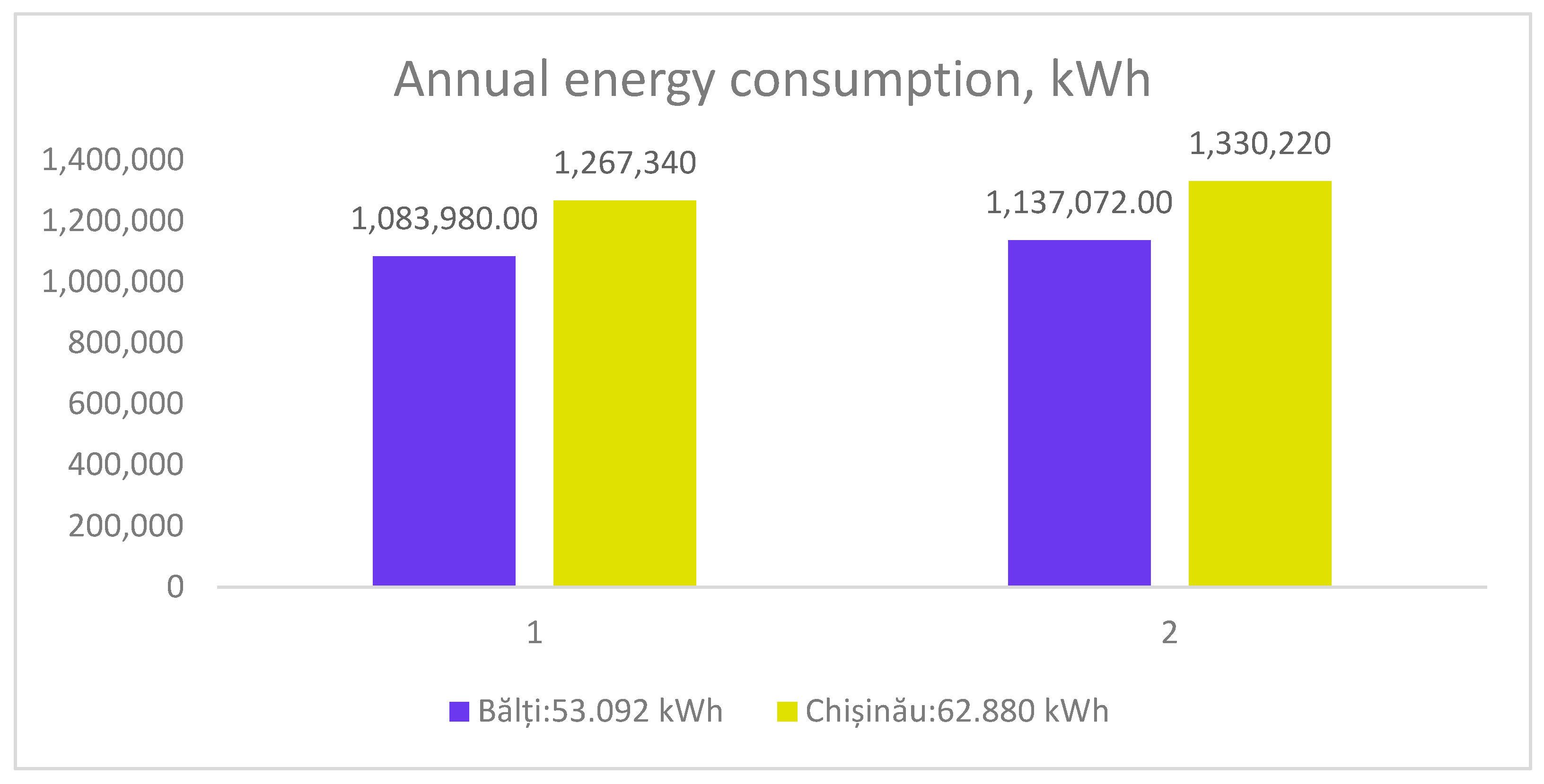
| Supermarket | Annual Energy Consumption, kWh |
|---|---|
| Bălți | 1,083,980 |
| Chișinău | 1,267,340 |
| Supermarket | Measured Annual Energy Consumption, kWh |
|---|---|
| Bălți | 1,137,072 |
| Chișinău | 1,330,220 |
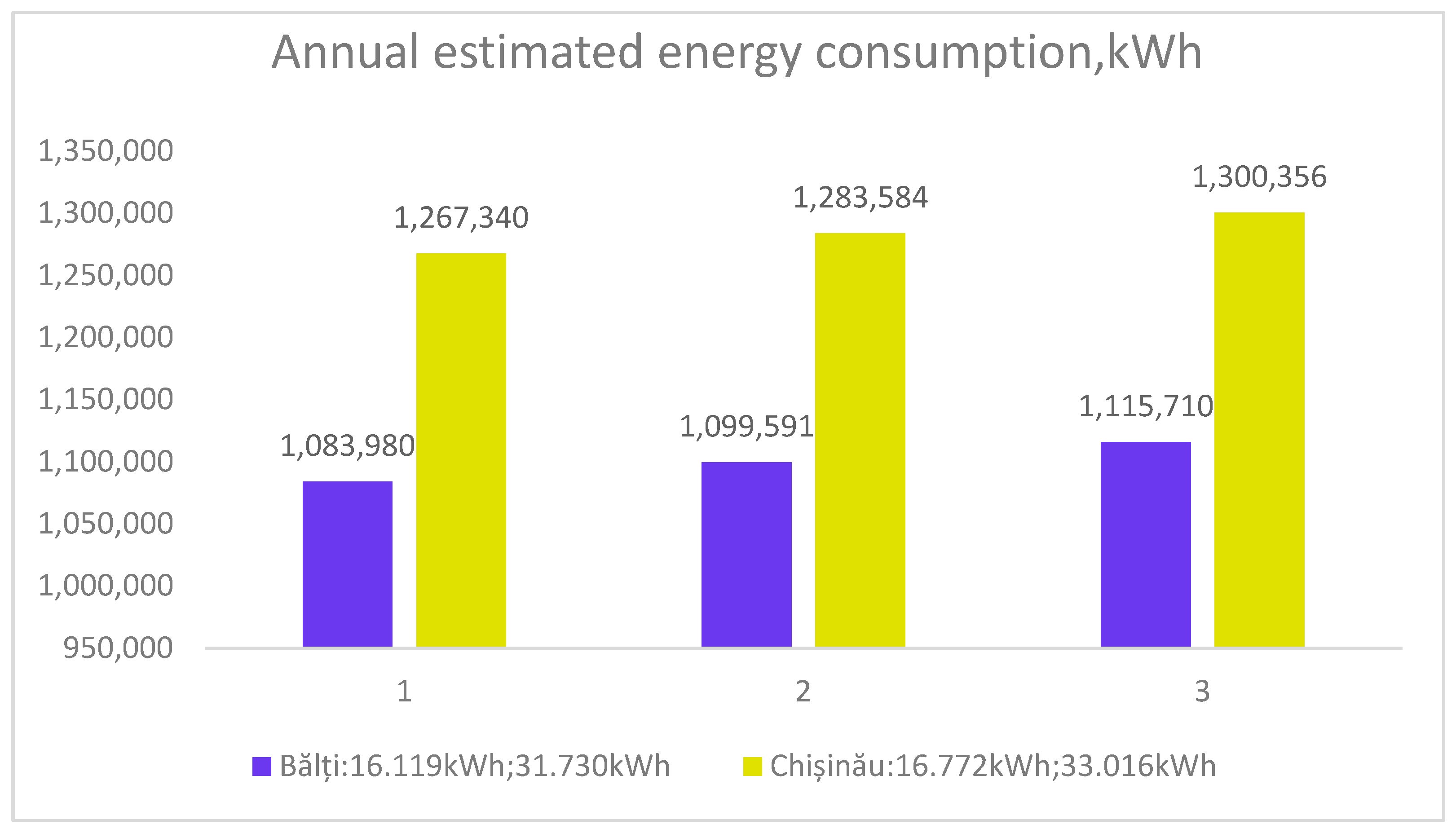
| Supermarket | Annual Energy Consumption | |
|---|---|---|
| kWh | % | |
| Bălți | 1,083,980 increased to 1,099,591 | 1.44 |
| Chișinău | 1,267,340 increased to 1,283,584 | 1.28 |
| Supermarket | Annual Energy Consumption | |
|---|---|---|
| kWh | % | |
| Bălți | 1,083,980 increased to 1,115,710 | 2.93 |
| Chișinău | 1,267,340 increased to 1,300,356 | 2.61 |
Disclaimer/Publisher’s Note: The statements, opinions and data contained in all publications are solely those of the individual author(s) and contributor(s) and not of MDPI and/or the editor(s). MDPI and/or the editor(s) disclaim responsibility for any injury to people or property resulting from any ideas, methods, instructions or products referred to in the content. |
© 2025 by the authors. Licensee MDPI, Basel, Switzerland. This article is an open access article distributed under the terms and conditions of the Creative Commons Attribution (CC BY) license (https://creativecommons.org/licenses/by/4.0/).
Share and Cite
Dumitriu, I.; Ion, I.V. Influence of Operating Conditions on the Energy Consumption of CO2 Supermarket Refrigeration Systems. Processes 2025, 13, 2138. https://doi.org/10.3390/pr13072138
Dumitriu I, Ion IV. Influence of Operating Conditions on the Energy Consumption of CO2 Supermarket Refrigeration Systems. Processes. 2025; 13(7):2138. https://doi.org/10.3390/pr13072138
Chicago/Turabian StyleDumitriu, Ionuț, and Ion V. Ion. 2025. "Influence of Operating Conditions on the Energy Consumption of CO2 Supermarket Refrigeration Systems" Processes 13, no. 7: 2138. https://doi.org/10.3390/pr13072138
APA StyleDumitriu, I., & Ion, I. V. (2025). Influence of Operating Conditions on the Energy Consumption of CO2 Supermarket Refrigeration Systems. Processes, 13(7), 2138. https://doi.org/10.3390/pr13072138