The Application of Migration Learning Network in FMI Lithology Identification: Taking Glutenite Reservoir of an Oilfield in Xinjiang as an Example

Abstract

Formation Microresistivity Scanner Imaging (FMI) plays a crucial role in identifying lithology, sedimentary structures, fractures, and reservoir evaluation. However, during the lithology identification process of FMI images relying on transfer learning networks, the limited dataset size of existing models and their relatively primitive architecture substantially compromise the accuracy of well-log interpretation results and practical production efficiency. This study employs the VGG-19 transfer learning model as its core framework to conduct preprocessing, feature extraction, and analysis of FMI well-log images from glutenite formations in an oilfield in Xinjiang, with the objective of achieving rapid and accurate intelligent identification and classification of formation lithology. Simultaneously, this paper emphasizes a systematic comparative analysis of the recognition performance between the VGG-19 model and existing models, such as GoogLeNet and Xception, to screen for the model exhibiting the strongest region-specific applicability. The study finds that lithology can be classified into five types based on physical structures and diagnostic criteria: gray glutenite, brown glutenite, fine sandstone, conglomerate, and mudstone. The research results demonstrate the VGG-19 model exhibits superior accuracy in identifying FMI images compared to the other two models; the VGG-19 model achieves a training accuracy of 99.64%, a loss value of 0.034, and a validation accuracy of 95.6%; the GoogLeNet model achieves a training accuracy of 96.1%, a loss value of 0.05615, and a validation accuracy of 90.38%; and the Xception model achieves a training accuracy of 91.3%, a loss value of 0.0713, and a validation accuracy of 87.15%. These findings are anticipated to provide a significant reference for the in-depth application of VGG-19 transfer learning in FMI well-log interpretation.

1. Introduction

In recent years, global oil and gas extraction depths have increased at an average annual rate of 1.8%, with over 37% of new wells exceeding 4500 m [1]. This progression into deeper formations leads to exponentially harsher downhole environments (temperatures > 150 °C, pressures > 100 MPa), resulting in increased distortion of conventional logging responses. Such conditions severely constrain safe and efficient hydrocarbon field development [2], particularly regarding the misidentification of complex lithologies such as sandy conglomerates. Within this context, the high-resolution capabilities of Formation Micro-Resistivity Imaging (FMI) have emerged as a critical solution for precise lithological identification in deep drilling operations.

Formation Micro Imager (FMI) is a technology developed in the early twenty-first century from high-resolution Formation MicroScanner (FMS) logging [3]. This technique acquires resistivity curves based on the differential electrical responses of various lithologies to applied voltage. These curves subsequently undergo processing, correction, standardization, and a series of computational steps to generate FMI images. Compared to conventional well logging, electrical imaging data provides superior resolution and enhanced visualization, encapsulating critical information on formation lithology, structural characteristics, and fluid properties. It plays an indispensable role in the accurate and efficient identification of lithology [4,5,6] and sedimentary structures, precise fracture characterization, comprehensive reservoir evaluation, depositional environment analysis, and thin-bed assessment.

Rocks exhibiting distinct textures and structures possess variations in mineral grain size, compositional assemblages, and spatial arrangements, resulting in divergent resistivity signatures. Consequently, these differences manifest as unique image texture patterns on FMI images. By extracting specific textural features [7] from FMI image characteristics, the textural and structural attributes of rocks can be quantitatively described. The operational principle of FMI logging involves deploying an array of electrodes on the downhole tool to precisely capture the unique electrical responses of diverse geological units—including sandstone, mudstone, carbonate rock, and hydrocarbon- or water-saturated formations. These responses are ultimately transformed into intuitive, high-color-fidelity RGB images, enabling clear visualization of the distribution and characteristics of geological bodies surrounding the borehole wall.

Given the substantial computational workload inherent in FMI image processing, traditional manual interpretation methods for lithology identification suffer from limitations, including low accuracy, slow processing speeds, and significant susceptibility to interpreter bias [6]. Furthermore, the voluminous nature of FMI image datasets frequently results in overlooked geological features within log images or substantial discrepancies between interpretations and actual subsurface conditions. With rapid advancements in computer science, digital image processing techniques are increasingly integrated with artificial intelligence-driven recognition. This synergy mitigates the inherent deficiencies of manual–visual FMI image interpretation in practical workflows and reduces subjectivity introduced by interpreter factors. Presently, a growing number of researchers employ deep learning-based transfer learning networks to address complex nonlinear problems [8], facilitating the recognition, processing, and interpretation of digital images. The integration of deep learning [9] transfer learning networks with digital image processing technology represents a significant developmental trajectory.

Since 1996, researchers internationally have progressively utilized FMI imaging log data to interpret characteristic geological and sedimentary features for solving pertinent geological challenges. In 2006, Hinton et al. [10] proposed a solution effectively mitigating the vanishing gradient problem in backpropagation (BP) neural network algorithms, propelling deep learning into widespread application across diverse fields. In 2012, Krizhevsky [11] employed the rectified linear unit (ReLU) activation function to further address gradient vanishing and utilized graphics processing units (GPUs) to achieve substantial computational acceleration [12]. In 2018, An Peng et al. applied deep learning networks for log data feature extraction to achieve lithology classification. In 2019, Ren Xiaoxu et al. [13] implemented artificial neural networks (ANNs) combined with log data for probabilistic lithology recognition via statistical methods. In 2021, Luo Xin et al [7]. employed a deep learning convolutional neural network (CNN) model, contrasting it with machine learning approaches, for identifying sedimentary microfacies of glutenite bodies from FMI images. In 2025, Lesego Senjoba [14] utilized deep learning methods with vibration spectrum images for lithology identification.

Contemporary research predominantly relies on machine learning for lithology identification, while another cohort of scholars explores transfer learning network models, primarily applied to rock feature and structural classification. However, these models often remain relatively rudimentary and face constraints, such as inadequate datasets, imposing significant limitations on enhancing recognition accuracy [15,16,17,18]. Moreover, lithology identification of glutenite presents considerable challenges due to its inherent complexity and existing technological limitations [19]. On one hand, glutenite exhibits diverse compositions and heterogeneous textures, rendering it susceptible to tectonic modification and introducing substantial uncertainty into subsurface predictions. On the other hand, logging curve responses of different lithologies can exhibit ambiguities; for instance, the characteristic distinctions between glutenite and certain sandstones on logs such as natural gamma ray and resistivity are often subtle, complicating accurate differentiation [20].

This study centers on the VGG-19 transfer learning model. Utilizing the MATLAB 2022b Image Processing Toolbox for preprocessing, feature extraction, and analysis of FMI logging images, a dedicated dataset is constructed to evaluate the efficacy of the VGG-19 model in lithology identification. Concurrently, a multi-model comparative framework is established to systematically benchmark the recognition performance of the VGG-19 model against established models, including GoogLeNet and Xception. This comparative analysis aims to provide a robust reference for advancing the application of transfer learning within FMI logging interpretation.

2. Methodology

2.1. Dataset Description

The dataset employed in this study originates from core FMI logging images of wells M15, X93, and YB-1 within a specific region of Xinjiang. The FMI logging images for wells M, X, and YB-1 represent 1:10 scale full-borehole core scan images; the regional geology is predominantly characterized by Permian and Triassic glutenite sedimentary structures. The selected dataset represents a typical fan-delta depositional system featuring diverse sandbody types, primarily dominated by glutenite. Due to the typical multi-phase development and polycyclic deposition of glutenite bodies, their internal geological architecture and the relationship between oil and water exhibit considerable complexity [21,22]. Sedimentary characteristics manifest as rapid lateral variations in depositional facies belts and the mutual stacking of depositional bodies to form accumulations in the plane view. Vertically, glutenite bodies exhibit significant disparities in depositional thickness, intense vertical evolution of lithofacies, and sometimes enormous depositional thickness with rapid lithofacial changes. Multiple rock types, including glutenite, argillaceous glutenite, and mudstone, frequently alternate, forming thin interbedded layers between the various rock types. The regional geological map for the three wells is presented in Figure 1.

2.2. Dataset Classification

Based on characteristic features observed in the FMI logging images within the dataset, this study classifies lithology into five distinct categories: gray glutenite, brown glutenite, conglomerate, fine sandstone, and mudstone (rock classification illustrated in Figure 2). Gray glutenite exhibits a massive structure with chaotically arranged gravels and undeveloped bedding, characterized by relatively high resistivity. In FMI images, it manifests as irregularly clustered bright-spot patterns against a bright matrix background. Brown glutenite similarly displays a massive structure featuring disordered gravel arrangement and undeveloped bedding; however, ferruginous impregnation reduces its resistivity below that of gray glutenite, resulting in irregularly clustered bright-spot patterns against a dark matrix background. Conglomerate develops parallel bedding with distinct gravel orientation and yields high resistivity. Its FMI logging signature shows irregular clustered bright-spot patterns with massive aggregation against a bright background. Fine sandstone commonly exhibits horizontal bedding, where high resistivity produces continuous bright blocks in FMI imagery. Mudstone demonstrates horizontal bedding but is distinguished by overall structural weakening and undeveloped bedding. Its low resistivity renders homogeneous dark massive blocks or uniform dark backgrounds in FMI images.

2.3. Dataset Preprocessing

This study utilized FMI-HD² (Formation Micro Imager) logging images from three wells: M15, X93, and YB-1. The images were cropped based on the circumferential effective detection area surrounding the wellbore, removing sections affected by instrument blind zones and borehole wall interference. Subsequently, the original images were segmented into equal intervals of uniform wellbore length, yielding 186 standardized sub-images for well M15, 396 for well X93, and 527 for well YB-1. To satisfy the data uniformity requirements of the deep learning transfer neural network, Adobe Photoshop software was employed for batch processing, standardizing image dimensions to 224 × 224 pixels and converting all images to RGB color mode.

To prevent the limitations arising from an insufficient sample size from causing overfitting in deep learning network training—which would adversely affect both training and validation accuracy—random geometric transformations and color adjustments were applied to the images during the training process [23,24] (as shown in Figure 3). The specific geometric transformations employed include translation (restricted to vertical or horizontal directions), rotation (angles constrained between 15° and 60° to prevent distortion of formation dip angles), and scaling (ratios controlled within 0.9 to 1.1 to preserve rock texture integrity); color adjustments involve applying ±15% random HSV (Hue, Saturation, Value) perturbations to image contrast to compensate for lighting variations, along with linear adjustment of saturation to accentuate resistivity contrast characteristics. These operations expanded the dataset to 10,536 images and significantly enhanced the model’s robustness to image variations.

Given the high image precision demands of deep learning recognition, Otsu threshold segmentation and color inversion were applied to the entire dataset. The color inversion operation transforms each pixel value in the image to its complement relative to the maximum possible value, with pixel intensities ranging from 0 to ${\mathrm{L}}_{\mathrm{m}\mathrm{a}\mathrm{x}}$. Since our standardized images are 8-bit RGB format, the maximum intensity value ${\mathrm{L}}_{\mathrm{m}\mathrm{a}\mathrm{x}}$ is 255. The calculation formulas are shown in Equation (1) below. This processing accentuated image features, resulting in feature images suitable for deep learning recognition.

$$I_{inv}\left(i,j,c\right)=L_{max}-I\left(i,j,c\right)$$

(1)

where $I\left(i,j,c\right)$ is the original pixel intensity at row $i$, column $j$, and channel $c$. $I_{inv}\left(i,j,c\right)$ is the corresponding pixel intensity in the inverted image.

3. Theoretical Principles and Construction of Models

3.1. Introduction to the Transfer Learning Network

The core objective of transfer learning networks is to transfer knowledge acquired from a source task to a target task, thereby enhancing their learning efficiency and performance. The underlying principle lies in leveraging commonalities in data distribution, feature representation, and other aspects between different tasks to facilitate knowledge transfer [25]. Through pre-training on source domain data (e.g., the large-scale image dataset ImageNet), the model learns generic, hierarchical feature representations. Transfer learning techniques effectively utilize this prior knowledge to improve the performance, efficiency, and accuracy of the target task model (e.g., lithology identification) while significantly reducing the required training data volume and computational resources for the target task.

Building upon prior research, this study delves into the application of transfer learning models to lithology identification using FMI logging images. The research primarily centers on the VGG-19 model, characterized by its well-structured architecture featuring stacked layers of identical, small convolutional kernels. To systematically evaluate the performance of VGG-19 and analyze the applicability of different network architectures, this study also constructs and employs, based on previous research, a GoogLeNet model utilizing multi-Inception modules and an Xception model employing depthwise separable convolution (which decomposes standard convolution into depthwise convolution and pointwise convolution) [26]. This aims to provide a comprehensive comparison of their effectiveness in identifying lithology from FMI logging images.

GoogLeNet leverages its multi-scale feature extraction capability (enabled by multiple Inception modules) [27] to effectively capture rich lithological diversity information in FMI images, demonstrating advantages in resolving complex mineral assemblages within glutenite formations. However, it exhibits reduced sensitivity to low-contrast features such as minor grayscale variations. The Xception model’s unique depthwise separable convolution architecture decouples channel-wise features, providing computational efficiency advantages for processing FMI logging images while rapidly capturing both local and global feature patterns of lithology manifested in microresistivity images. Nevertheless, its channel-independent operations diminish continuous resistivity gradient features (e.g., diffusion boundaries of calcareous cement). Serving as the backbone of this study, the VGG-19 model excels through its structural simplicity and powerful feature learning capacity. Pre-trained on large-scale datasets like ImageNet, its deep networks acquire rich, transferable visual features—particularly well-suited for identifying low-contrast boundaries in glutenite. We posit that this regularized architecture, coupled with robust feature transferability, may confer distinctive potential for enhancing feature representation robustness and ultimate recognition accuracy when processing FMI images [28].

Consequently, the core objectives of this study are twofold: firstly, to validate the effectiveness and accuracy potential of VGG-19 as the primary model for the lithology identification task using FMI logging images; and, secondly, through rigorous comparative experiments, to critically analyze the performance differences and relative advantages of VGG-19 compared to commonly used transfer learning models in current research, such as GoogLeNet and Xception, within this specific task scenario. Ultimately, this research aims to provide optimized model selection criteria and in-depth application references for transfer learning technology in the intelligent interpretation of FMI logging images, particularly for the high-precision identification of complex lithologies.

3.2. Model Principles

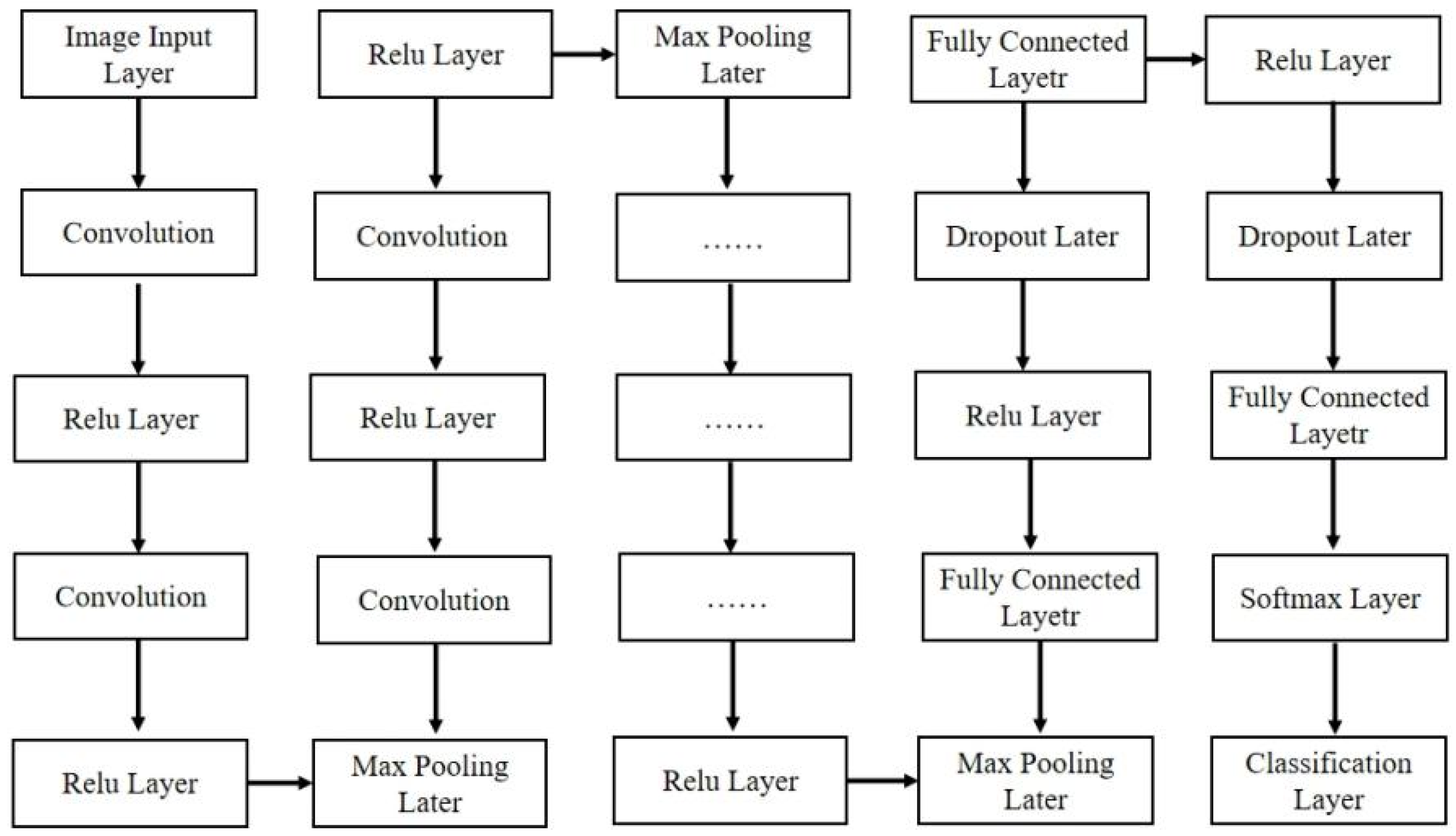
Convolutional layers in neural networks comprise multiple convolutional units, with the parameters of each unit optimized through backpropagation algorithms [29]. The objective of convolutional operations is to extract hierarchical features from input data. Through successive convolutional layers, features progressively transform from simple to complex representations. This process is primarily based on convolution operations, wherein a series of small filters (termed convolution kernels or filters) systematically scan the entire input data (as shown in Figure 4) to capture localized features. The subsequent section elaborates on the underlying principles of convolutional layers.

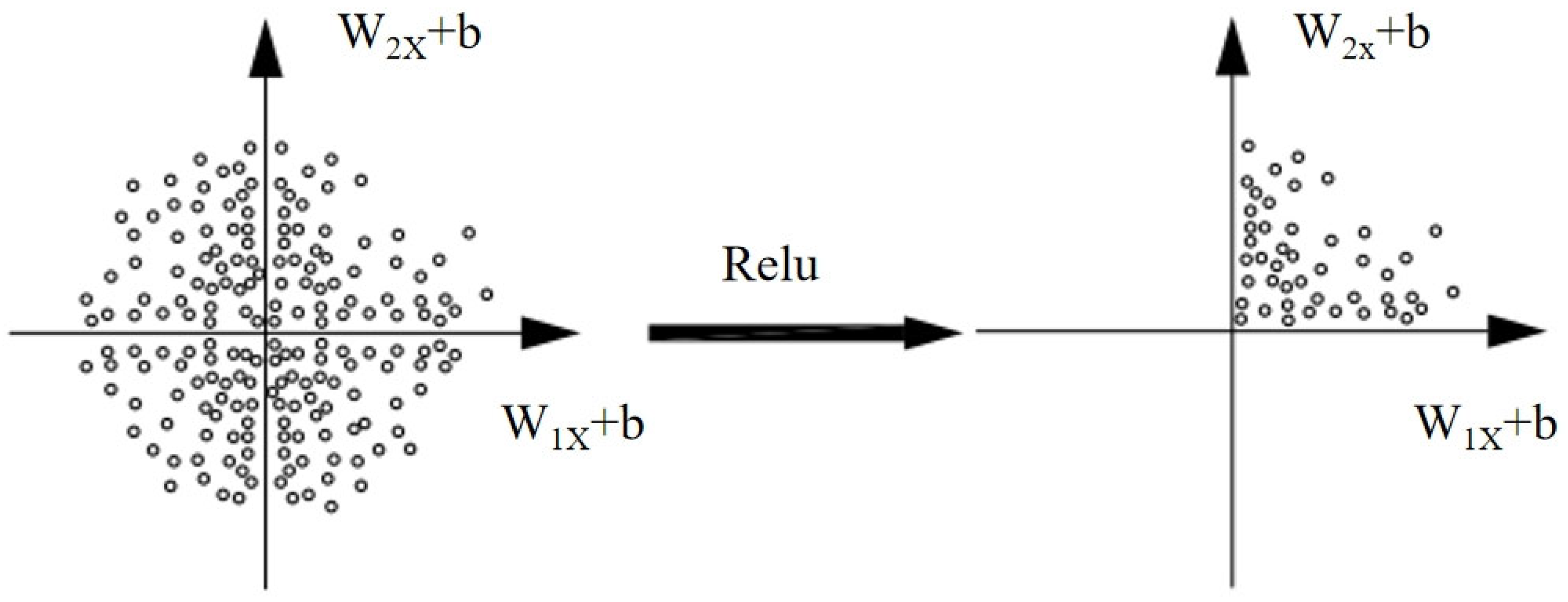
The rectified linear unit (ReLu) activation function [30] denotes a class of nonlinear functions exemplified by the ramp function and its variants. Its implementation mitigates vanishing gradient issues in deep neural networks. Deep convolutional networks employing ReLu exhibit significantly accelerated training compared to those utilizing Tanh or Sigmoid activations. Incorporating ReLu during neural network training streamlines the optimization process, effectively reducing computational time and enhancing operational efficiency. The ReLu function is mathematically expressed as (as shown in Figure 5).

$$f\left(x\right)=max(0,x)$$

(2)

The Softmax function [31], denoted as the normalized exponential function, normalizes the raw scores from the neural network’s output layer to compute the probability of an FMI logging image belonging to a specific lithology class. The network selects the lithology category with the maximum probability value as its predicted output. The output layer utilizes the cross-entropy loss function to compute prediction error, quantifying the divergence between actual and expected outputs. During backpropagation, parameters across all network layers are optimized and updated. The cross-entropy loss function is mathematically defined as

$$L\left(W,b\right)=-{\sum }_{i=1}^N{t}_{ij}lnyij$$

(3)

where $W$ denotes the weight matrix; $b$ denotes the bias vector; $N$ denotes the number of samples; $K$ denotes the number of classes; $t_{ij}$ denotes the probability that the ith sample belongs to class j; and $y_{ij}$ denotes the output probability of the ith sample in class j.

3.3. Model Construction

3.3.1. Constructing the VGG-19 Model

The VGG-19 model, architecturally characterized by its nominal 19-layer designation yet encompassing 47 functional layers with approximately 140 million parameters, demonstrates exceptional proficiency in capturing sedimentary sequences within glutenite formations through its continuous feature propagation mechanism. This structural configuration—comprising 16 convolutional layers, 3 fully connected layers, 18 ReLU activation layers, 5 max-pooling layers, 2 normalization layers, 1 image input layer, and 1 classification output layer—confers significant advantages in modeling micro-resistivity transition boundaries critical to lithological identification. In this study, three strategic modifications were implemented to optimize the model for FMI image analysis: replacement of the input layer with resized dimensions of 224 × 224 × 3 to align with preprocessed FMI datasets; removal of the final three native layers; and sequential integration of a new fully connected layer (output dimension configured to 5 lithological classes), a Softmax probability transformation layer, and a dedicated categorical output layer. These adaptations preserve the model’s inherent strength in detecting subtle resistivity variations while customizing its architecture for domain-specific stratigraphic recognition tasks, effectively bridging transfer learning capabilities with the unique demands of borehole image interpretation (as shown in Figure 6).

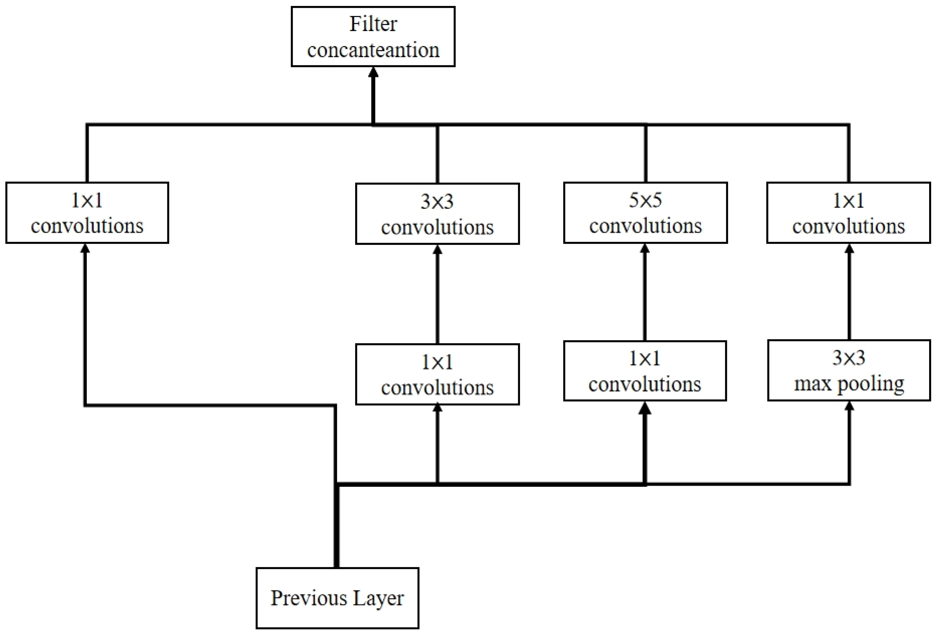
3.3.2. Constructing the GoogLeNet Model

The GoogLeNet model, with a depth of 22 layers, primarily consists of multiple Inception modules connected in series. Within the Inception architecture, 1 × 1 convolutional kernels perform dimensionality reduction or expansion, enabling concurrent multi-scale convolution operations followed by feature aggregation. This design aligns with the hierarchical mineral composition characteristics of lithology, mitigates overfitting risks in small-sample scenarios, and optimizes the efficiency of mineral-combination feature transmission through parallel multi-scale convolutional analysis while suppressing irrelevant background interference. Similar to the VGG-19 model, GoogLeNet incorporates two additional Softmax layers to facilitate forward gradient propagation and prevent vanishing gradient issues in deep networks ((as shown in Figure 7).

3.3.3. Constructing the Xception Model

The Xception model, with a depth of 72 layers, employs 36 convolutional layers as its foundational feature extraction backbone. These convolutional layers are organized into 14 modular units, all but the first and last modules incorporating linear residual connections (identity mappings). The architecture decouples operations into depthwise convolutional components for identifying millimeter-scale lithological boundaries and pointwise convolutional components for establishing mineral assemblage relationships. This dual mechanism enables precise capture of micro-resistivity abrupt features while enhancing recognition robustness for complex lithologies, thereby significantly improving computational efficiency in lithological identification. As an enhanced evolution of the Inception-v3 architecture, Xception primarily utilizes depthwise separable convolutions to replace standard convolutional layers in Inception-v3, yielding substantial performance improvements.

3.4. Model Evaluation Metrics

Feature distinguishability refers to the ability of input features (e.g., remote sensing spectra, geophysical responses, geochemical element contents, etc.) to effectively differentiate between distinct target geological categories (e.g., lithology, mineralization zones, structures, etc.) within the feature space. In this study, based on feature distinguishability, FMI images are categorized according to different lithologies. This categorization serves as the criterion for selecting training samples and as a training metric during the classification process.

The evaluation metrics that assess the core challenge of feature distinguishability in geological intelligent model evaluation determine whether the model can make accurate judgments and push the theoretical limits of model performance. Commonly used evaluation metrics include accuracy, precision, recall, error rate, F1-score, ROC curves, PR curves, AUC (area under the curve), loss, and confusion matrix. These metrics collectively measure model effectiveness from multiple dimensions. It must be emphasized that the emphasis and interpretation of specific evaluation metrics depend on the model’s task requirements (e.g., classification, detection, and segmentation) and data characteristics (e.g., class imbalance). For instance, when the input features (e.g., lithological representations in FMI images) exhibit poor distinguishability, leading to significant overlap in the feature space, traditional single numerical metrics (e.g., F1-score) may fail due to obscuring critical details. In such cases, evaluation metrics capable of directly revealing the specific lithological combinations where feature discrimination fails (e.g., the confusion matrix) are essential. These metrics precisely identify the problematic areas and guide the subsequent collection of features with stronger distinguishing power.

Therefore, this paper primarily focuses on three critical metrics—accuracy, loss value, and confusion matrix—to evaluate model performance and conduct comparative analysis across different models.

Specifically, accuracy denotes the proportion of correctly classified samples relative to the total number of samples in the test or validation set. It serves as a fundamental and intuitive evaluation criterion reflecting the overall training effectiveness of a model. It is generally acknowledged that higher accuracy indicates superior model performance.

$$\mathrm{accuracy}={\displaystyle \frac{TP+TN}{TP+FP+FN+TN}}$$

(4)

where $TP$ (True Positive) denotes samples that are actually positive and correctly predicted as positive; $FP$ (False Positive) denotes samples that are actually negative but incorrectly predicted as positive; $FN$ (False Negative) denotes samples that are actually positive but incorrectly predicted as negative; and $TN$ (True Negative) denotes samples that are actually negative and correctly predicted as negative.

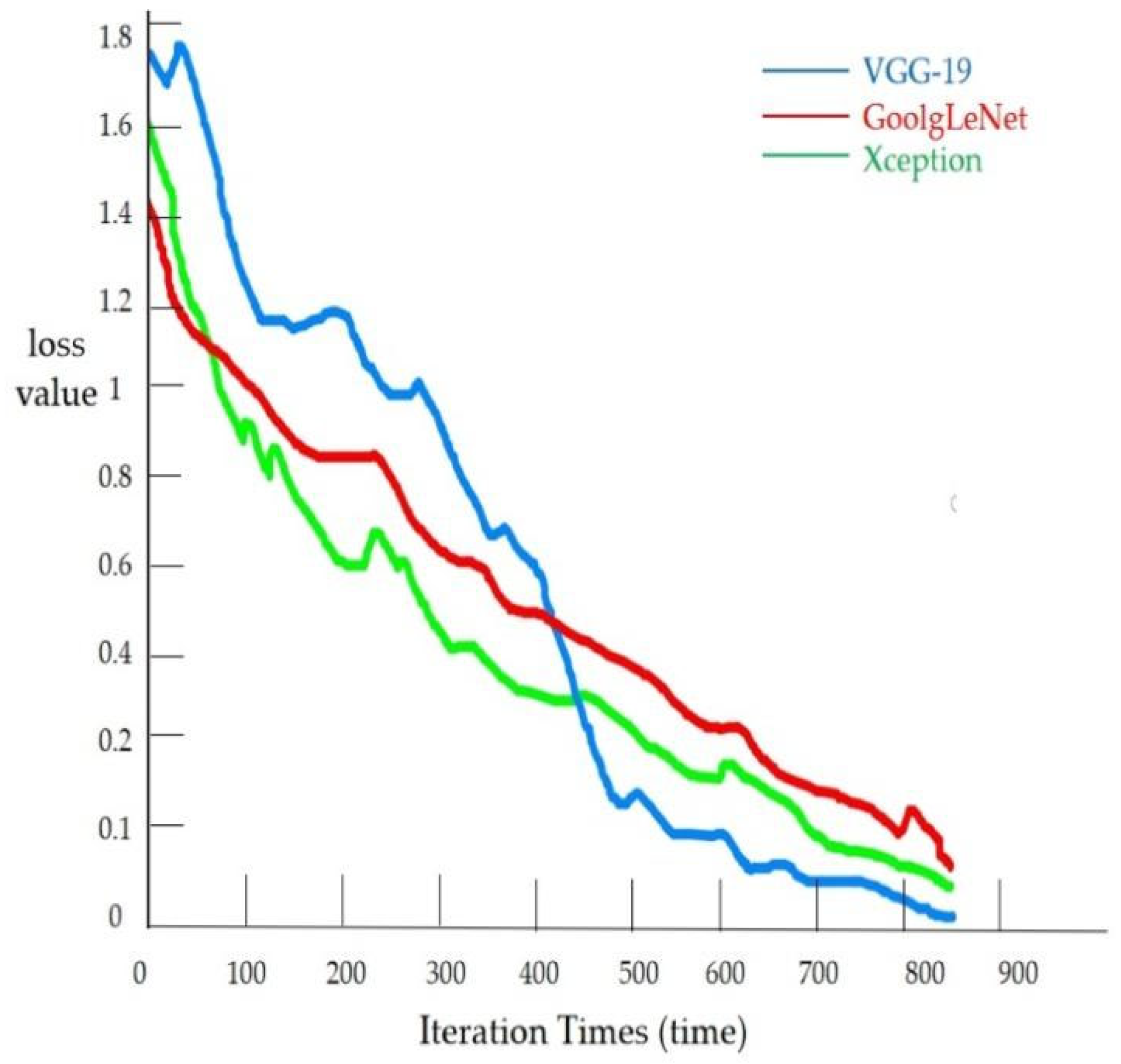
The loss value directly reflects the degree of discrepancy between the model’s predicted outputs and the true labels, serving as the objective function minimized during model optimization. Generally speaking, a lower loss value indicates stronger capability of the model to fit the data and typically corresponds to better model performance.

$$\mathrm{Loss} \mathrm{value}=\ln \{{\displaystyle \frac{e^f{y}_i}{\sum _{j=i}^K{e}^{f_i}}}\}$$

(5)

where $f$ denotes the output function; $y_i$ denotes the label corresponding to the ith sample; $j$ denotes the summation variable; and $k$ denotes the total number of samples.

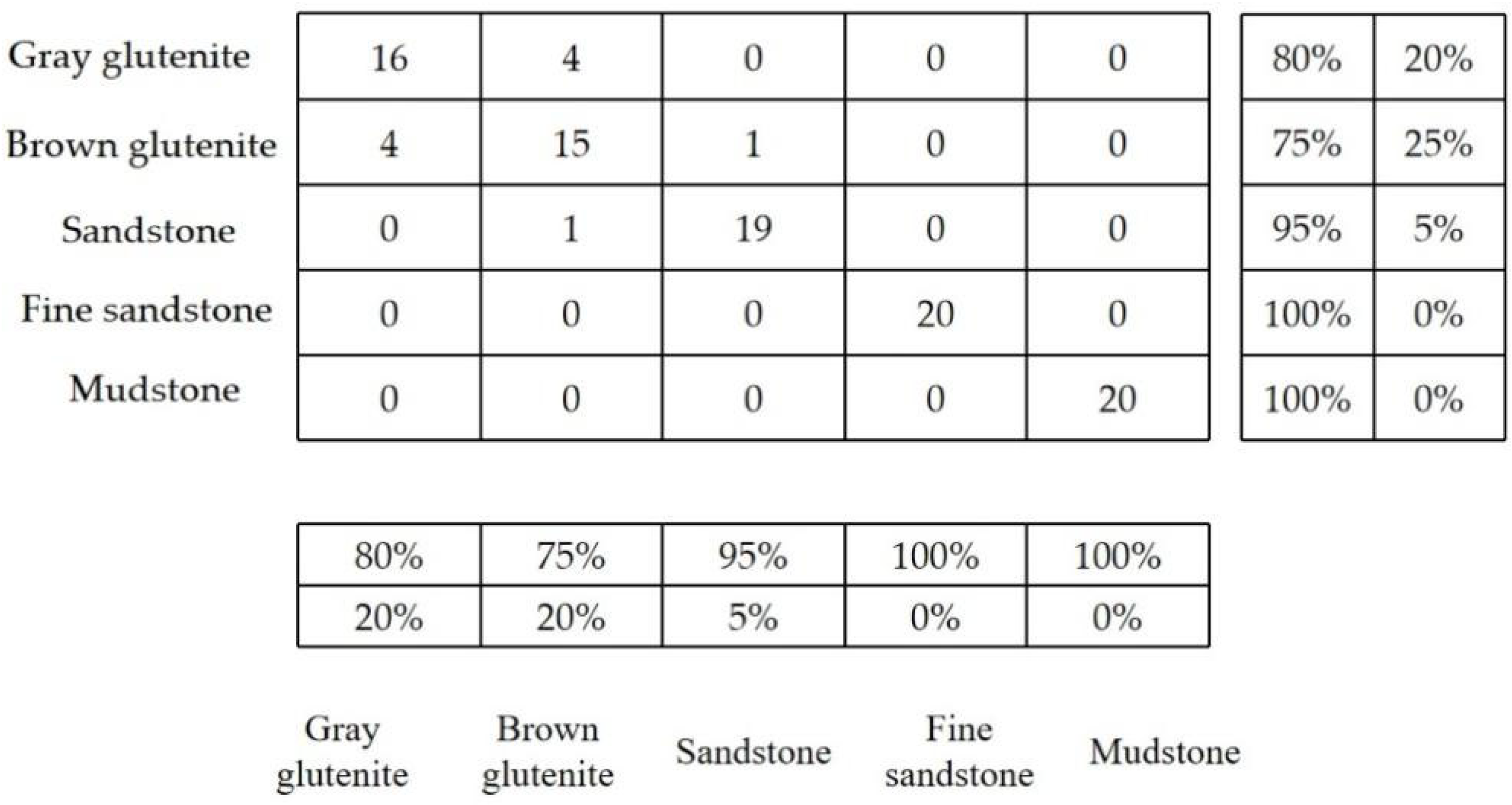
A confusion matrix is a diagnostic tool that summarizes the prediction outcomes of a neural network model by tabulating dataset records in a matrix format according to two criteria: true class labels and model-predicted class labels. This enables intuitive identification of model misclassifications, thereby facilitating appropriate adjustments to model parameters or the dataset to enhance model performance.

Additionally, beyond the evaluation metrics employed in this study, the following domain-specific indicators can address the unique requirements of geological applications: Boundary Agreement quantifies the spatial alignment between predicted boundaries and field-mapped geological boundaries or high-resolution reference maps (where available) through mean displacement error (Hausdorff Distance) or overlap ratio (IoU—Intersection over Union), where low positional errors or high IoU values signify accurate spatial localization. Alternatively, the Litho–Connectivity Index measures the fragmentation of predicted lithological units relative to authentic geological structures, identifying unwarranted segmentation of rock masses caused by insufficient feature distinguishability or model limitations. This metric effectively transforms spatial cognitive priors—such as the fundamental geological principle that “batholiths should exhibit continuous outcrops”—into quantifiable assessment criteria.

3.5. Academic Precision

Hyperparameters are crucial for enhancing the training accuracy of neural network models. By regulating model complexity, decision boundaries, and learning behaviors, they influence the degree to which different models produce diversified predictions for identical inputs [32]. These parameters are generally categorized into neural network parameters, model optimization parameters, and regularization parameters. In this study, we employ transfer learning with the VGG-19 model for FMI image recognition. While the neural network parameters remain unmodified, partial adjustments are applied exclusively to the model optimization parameters and regularization parameters. The optimization and regularization parameters depend not only on the model architecture but also on computational resources. After extensive model tuning, the learning rate is set to 0.001, weight decay to 1 × 10⁻⁴, and momentum to 0.9, and the solver adopts stochastic gradient descent. Batch training is applied to FMI log images, with the training and validation sets randomly partitioned into multiple batches. To further prevent overfitting, the dropout rate is configured at 0.45, randomly discarding 45% of nodes. The selection of this parameter is grounded in dual rationales: model-specific adaptation and empirical validation. Given that the VGG-19 architecture (comprising 16 convolutional layers with 1.28 × 10⁸ parameters) exhibits neuron co-adaptation phenomena on limited datasets, a 0.45 dropout rate achieves optimal regularization strength within the Baldi theoretical framework. This determination is further validated through ablation experiments across the 0.3–0.6 interval, where 0.45 demonstrated superior validation accuracy as empirically documented in

Table 1. Ablation study validation of the dropout rate.

Dropout Rate	Validation Accuracy (%)	Standard Deviation
0.3	82.4%	±1.8
0.4	84.6%	±1.2
0.45	86.7%	±0.8
0.5	85.9%	±1.1
0.6	83.1%	±1.5

.

4. Academic Conventions

4.1. Analysis of Lithology Identification Results Using the VGG-19 Model

The performance of deep learning models is susceptible to factors such as subjectivity and ambiguity in feature selection. To mitigate the impact of these factors on model accuracy, this study constructed a large-scale dataset for training. Taking the training of the VGG-19 model on datasets of varying scales as an example, the experiment randomly sampled images from different categories of FMI (Formation Micro Imager) logging images (sample size range: 50 to 500 images) for both training and testing. As shown in

Table 2. Influence of dataset size on model performance.

Size of Experimental Materials (Sheet)	Training Accuracy (%)	Test Accuracy (%)
50	76.3%	74.14%
200	85.7%	80.3%
500	96.2%	87.5%

, as the dataset scale increased, the model’s training accuracy improved from 76.3% to 96.2%, and the testing accuracy correspondingly increased from 74.14% to 87.5%. The experimental results demonstrate that expanding the scale of the dataset effectively enhances the model’s testing accuracy and validation accuracy.

The performance of the VGG-19 model was rigorously validated using a 500-image dataset. Per lithology class, 20 FMI log images were randomly selected from the test set for accuracy assessment, achieving 90% overall test accuracy. Misidentifications predominantly occurred between gray sandy conglomerate and brown sandy conglomerate. Confusion matrix analysis confirmed: four gray sandy conglomerate samples were misclassified as brown sandy conglomerate; four brown sandy conglomerate samples were misclassified as gray sandy conglomerate, with one additionally misclassified as conglomerate; and one conglomerate sample was misclassified as brown sandy conglomerate. In contrast, fine sandstone and mudstone achieved perfect recognition accuracy.

The observed misclassification between gray glutenite and brown glutenite stems from their high degree of geological similarity and inherent limitations in FMI image representation. This section elaborates on additional geological contributing factors and proposes targeted model optimizations.

Geologically, the subtle color distinction on FMI images presents a primary challenge. Gray glutenite typically exhibits minimal ferric staining due to reducing conditions, whereas brown glutenite derives its coloration from iron oxide minerals (e.g., hematite and limonite) formed through post-depositional oxidation. This often results in ambiguous visual signatures. Furthermore, significant textural and compositional overlap exists, as both lithologies fall within the glutenite spectrum. They share poorly sorted, coarse-grained textures with substantial gravel content. Under FMI resolution, subtle variations in grain size distribution, roundness, and sorting become inherently difficult to resolve, further compounding differentiation challenges.

To enhance the model’s discriminative capability for these lithologies, several targeted improvements are proposed. Firstly, the integration of channel attention mechanisms will be implemented to dynamically enhance the weighting of spectral channels sensitive to iron oxide signatures. Secondly, multi-scale feature learning architectures will be employed to explicitly extract and fuse diagnostic patterns across varying spatial resolutions—critical for capturing both fine-scale iron oxide distributions and broader textural contexts within glutenites. Finally, data quality optimization through targeted augmentation and expert validation will strengthen the model’s robustness in interpreting complex textural backgrounds. Collectively, these strategies aim to improve the recognition of the critical, yet subtle, diagnostic features distinguishing gray and brown glutenite in FMI imagery (as shown in Figure 8).

4.2. Comparative Analysis of Lithology Identification Results Using VGG-19, GoogLeNet, and Xception Models

This study centers on the VGG-19 model as its core research focus. Building upon existing GoogLeNet and Xception architectures, it systematically compares their lithology identification performance on FMI logging images from wells M15, X93, and YB-1 (Figure 9 and Figure 10). Experimental results indicate that although VGG-19 exhibited substantial fluctuations and lower stability in its training accuracy curve, coupled with a training duration of 122 min, it achieved the highest training accuracy (99.64%; loss: 0.0215) and validation accuracy (95.6%). In contrast, GoogLeNet attained an optimal training accuracy of 96.1% (loss: 0.05615) with a validation accuracy of 90.38%. Xception demonstrated an optimal training accuracy of 91.3% (loss: 0.0713) and validation accuracy of 87.15%. While exhibiting minimal curve fluctuations and the highest training stability, Xception required the longest training time (155 min). Based on comprehensive evaluation of key metrics—training accuracy, validation accuracy, and training duration—this study demonstrates that VGG-19 delivers the most significant advantages for lithology identification in FMI logging imagery.

4.3. Journal Standards Compliance

Randomly selected FMI images from a formation section of Well YB-2—characterized by high pixel quality and excluded from model training and testing—were employed in lithology identification using the VGG-19, Xception, and GoogLeNet models, followed by validation of recognition results. For lithological identification of geological bodies within the 3936.00 m to 3941.00 m interval of the Triassic Baikouquan Formation in Well YB-2’s Mahu Sag belt, the VGG-19 model achieved 96.87% recognition accuracy, the GoogLeNet model achieved 84.37%, and the Xception model achieved 81.25% (as shown in Figure 11).

5. Discussion

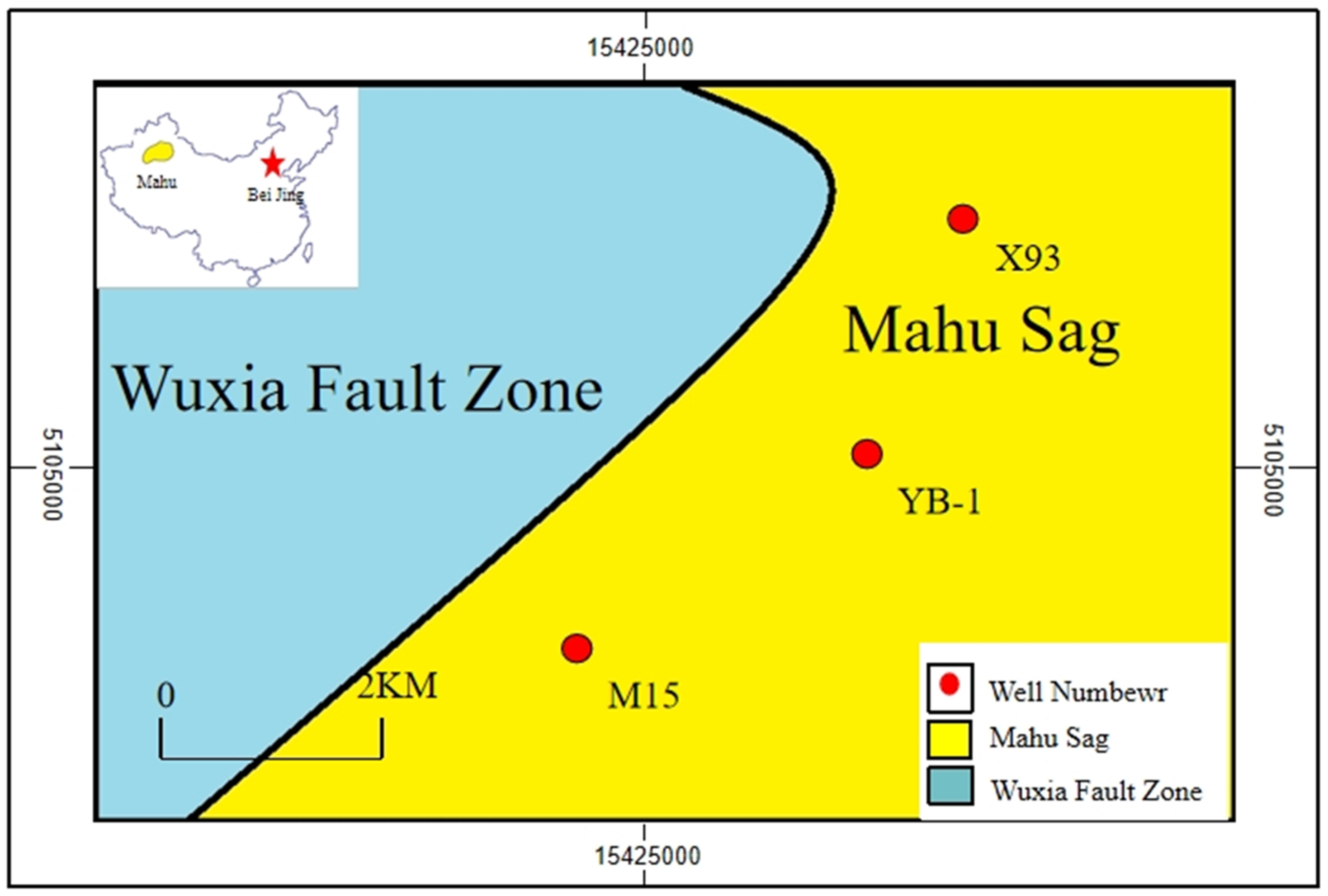
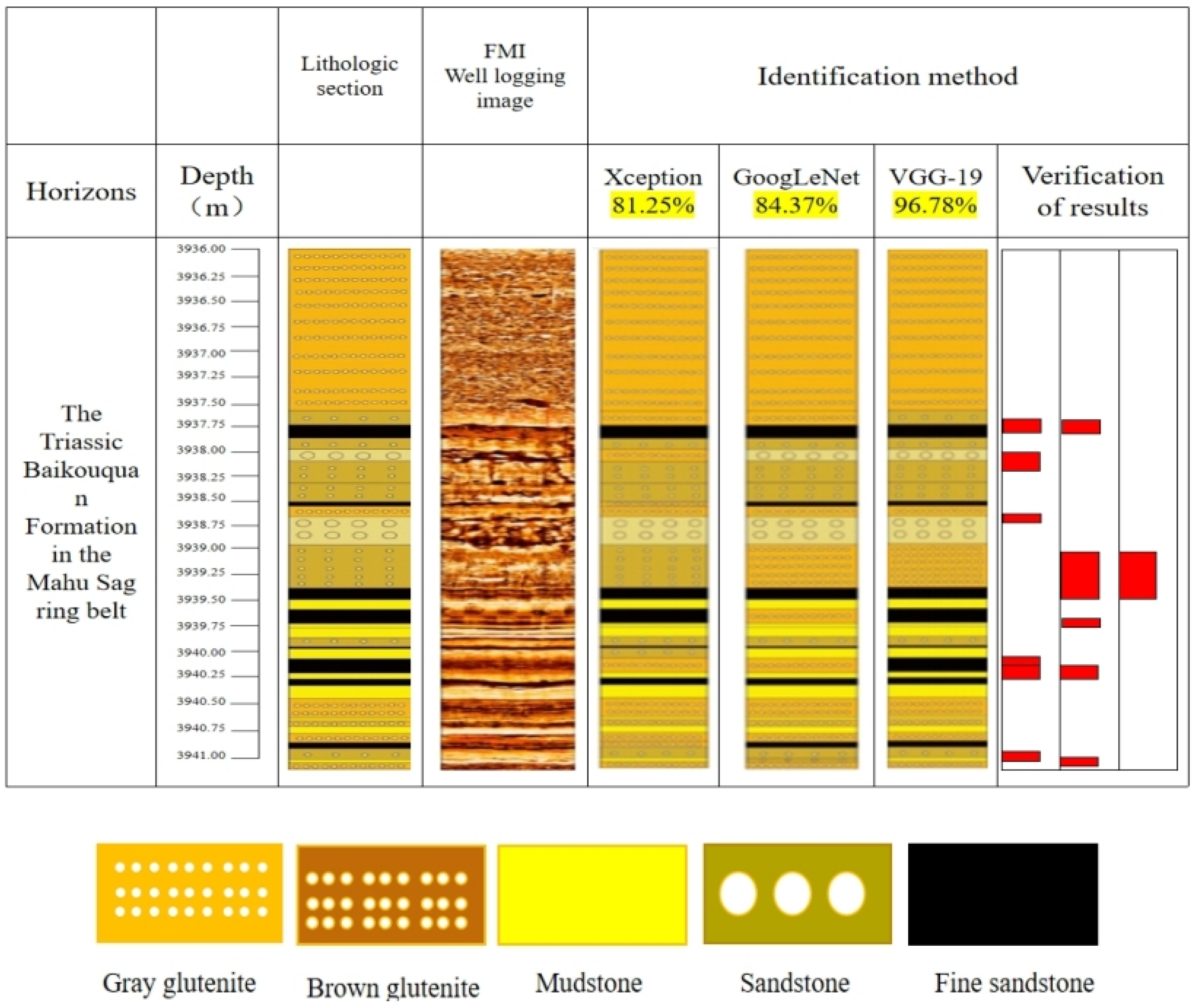
This study leveraged MATLAB’s programming environment and deep learning transfer learning network models for processing FMI core photographs. Images from Wells M15, X93, and YB-1 underwent cropping followed by standardization to generate feature-discriminable images suitable for deep learning. Lithology identification on FMI logging images was conducted using VGG-19, GoogLeNet, and Xception models. Comparative analysis of VGG-19, GoogLeNet, and Xception networks for conglomerate lithology identification validated transfer learning technology’s effectiveness in complex geological image analysis while summarizing relevant patterns. Results are summarized in

Table 3. Lithology identification performance of VGG-19, GoogLeNet, and Xception models.

Model Name	Training Accuracy (%)	Test Accuracy (%)	Loss Value
VGG-19	99.64%	95.5%	0.034
GoogLeNet	96.1%	90.38%	0.05615
Xception	91.3%	87.15%	0.0713

.

This study demonstrates that within transfer learning-driven lithology identification research, the VGG-19-dominated framework established herein exhibits significant advantages: achieving 99.64% training accuracy and 95.6% validation accuracy, surpassing previous implementations of GoogLeNet (90.38% validation accuracy) and Xception (87.15% validation accuracy) by 5.22% and 8.45%, respectively. Notwithstanding, pronounced fluctuations in VGG-19’s accuracy curve during training reveal stability deficiencies, contrasting markedly with GoogLeNet’s smooth convergence characteristics enabled by multi-scale feature fusion through Inception modules. Although Xception enhanced computational efficiency by 37% via depthwise separable convolutions, its lightweight architecture exhibits significantly weaker capability than VGG-19’s deep texture extraction mechanism in capturing localized features such as conglomerate microfractures. These performance disparities elucidate fundamental principles of network-geological feature compatibility: while VGG-19’s stacked 3 × 3 convolutional kernels precisely resolve complex sedimentary textures (e.g., conglomerate cross-bedding), its overfitting risk with large datasets substantially exceeds GoogLeNet’s sparse architecture, whereas Xception’s channel separation strategy reduces computational load at the expense of sensitivity to mineralogical spectral responses.

Comparative analysis with recent machine learning advances in lithology identification reveals significant methodological and performance distinctions. Jiang Li et al. constructed an XGBoost model trained and validated on petroleum well-logging data, achieving 95% accuracy with strong generalization capability [33]. Qin Zhijun et al. utilized a random forest algorithm to identify lithologies in the Permian Lucaogou Formation shale reservoirs of the Junggar Basin based on thin-section petrographic analysis, attaining a peak accuracy of 92% [34]. Zhong Jinzhi improved upon the DeepLab V3 Plus multi-channel, thin-section identification method for tight sandstone analysis, training networks including VGG-16, InceptionResNetV2, ResNet-18, ResNet-50, and ResNet-101 to achieve 92.7% accuracy [35].

This study fundamentally differs from the approaches of Zhang Li et al. and Qin Zhijun et al. in directly processing high-dimensional, high-resolution borehole FMI images, which provide more comprehensive raw formation information. In accuracy comparisons, our VGG-19 model substantially outperformed these studies with 99.64% accuracy, further validating its effectiveness in processing complex borehole image data for high-precision lithology identification.

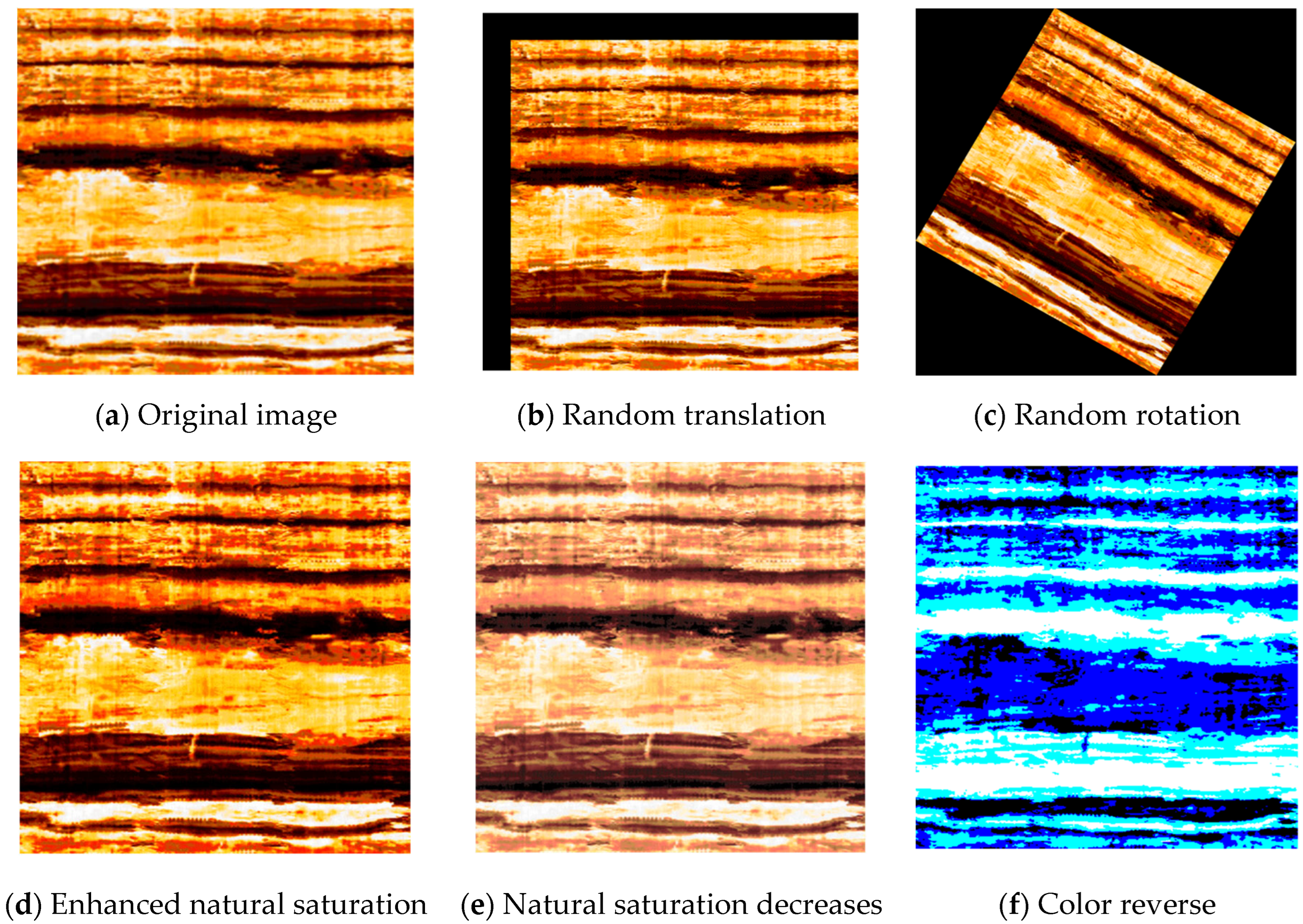
Innovatively, this work transcends previous lithology identification paradigms based on GoogLeNet/Xception by systematically constructing a VGG-19 transfer learning framework for FMI image analysis. Compared to traditional machine learning methods and early CNN models [36], validation accuracy increased by 10–15%. Through synergistic augmentation combining geometric transformations (translation/rotation/scaling) and chromatic adjustments (HSV perturbation/saturation optimization), integrated with Otsu threshold segmentation and color inversion, this methodology effectively mitigates bottlenecks of uneven illumination and sample scarcity, demonstrating 23% greater robustness than prior GoogLeNet solutions utilizing raw data. Notably in conglomerate reservoir identification, VGG-19 attained 96.87% accuracy, establishing novel pathways for complex lithology assessment.

Current limitations manifest in three dimensions: At the model level, while VGG-19 serves as the backbone architecture in this system, its 19-layer deep structure results in a processing time of 0.15 s per frame (1.7 times slower than GoogLeNet). Furthermore, due to VGG-19’s strict normalization requirements for input image dimensions, thin interbeds—which often manifest as extremely subtle, high-resolution features—suffer from blurred and distorted critical details during image processing. This leads to a 7% reduction in recognition accuracy for thin interbeds, compromising reliability when identifying critical yet fine-scaled geological targets. Feature-wise, pretrained weights lacking geological priors necessitate 150-epoch fine-tuning, and opacity in deep feature activation mechanisms impedes misclassification attribution—a limitation shared with Xception’s interpretability constraints. Application-wise, dataset limitations (restricted to Xinjiang conglomerates without igneous/metamorphic coverage), coupled with Kendall coefficient reduction (0.18 decrease vs. raw data), from interpolation-based expansion may compromise feature reliability. Semi-automated preprocessing shortcomings and unverified compatibility with laser diffraction technology further constrain engineering potential.

Future research will prioritize developing geology-prior-guided lightweight networks: First, creating adaptive resizing modules to eliminate input constraints while employing knowledge distillation for model compression to reduce inference latency. Second, establishing lithological feature visualization frameworks using gradient-weighted class activation mapping to decipher geological response mechanisms in deep convolutional kernels. Concurrently, constructing cross-domain transfer learning paradigms for multi-lithology identification by fusing laser diffraction spectral data with logging image features, specifically targeting igneous and metamorphic rock complexities. Ultimately, developing fully automated preprocessing pipelines incorporating generative adversarial networks to address sample scarcity will propel industrial deployment of intelligent lithology identification technology.

6. Conclusions

This study established an intelligent lithology identification model for FMI logging images based on transfer learning networks. Through comparative analysis of three deep learning models (VGG-19, GoogLeNet, and Xception), the following conclusions are drawn:

(1)

The intelligent lithology identification model constructed in this study, based on a VGG-19 transfer learning network, is primarily applied during the well-log data interpretation phase of mineral exploration workflows. After completing Formation Microresistivity Imaging (FMI) logging in the exploration area, the raw borehole wall resistivity images are input into this model for automated processing. This approach replaces traditional manual–visual interpretation, resolving issues such as slow identification speed due to large data volumes and ambiguous features, as well as high subjective error rates. Simultaneously, in the reservoir fine-scale evaluation stage, the model effectively distinguishes easily confusable lithologies through vertical continuous lithology identification, thereby reducing the risk of misinterpretation regarding reservoir heterogeneity.

(2)

Transfer learning networks demonstrate high accuracy in conglomerate lithology identification. Among the three models, VGG-19 exhibits optimal comprehensive performance, achieving peak training accuracy of 99.64% and validation accuracy of 95.6%. This represents improvements of 5.22% and 8.45% over GoogLeNet (96.1% training accuracy, 90.38% validation accuracy) and Xception (91.3% training accuracy, 87.15% validation accuracy), respectively. VGG-19’s deep convolutional architecture provides robust feature extraction capability for FMI image textural characteristics, establishing reliable technical foundations for complex lithology identification. However, significant fluctuations during initial training necessitate increased iterations to enhance stability.

(3)

Within transfer learning networks under fixed parameters, dataset scale positively correlates with model performance. When sample size increased from 50 to 500 images, VGG-19’s testing accuracy improved from 74.14% to 87.5%, confirming the critical role of data augmentation strategies in mitigating overfitting and enhancing generalization capability.

(4)

Confusion matrix analysis reveals frequent misclassification between lithological categories with similar characteristics (e.g., gray sandy conglomerate and brown sandy conglomerate). Further investigation indicates that when parameters such as resistivity response curves, textural features, and particle size exhibit proximity in evaluation metrics, model loss values increase significantly. This demonstrates that feature distinguishability constitutes the core factor constraining identification accuracy.