Abstract
Formation MicroScanner Image (FMI) technology is a key method for identifying fractured reservoirs and optimizing oil and gas exploration, but its inherent insufficient resolution severely constrains the fine characterization of geological features. This study innovatively applies a Super-Resolution Generative Adversarial Network (SRGAN) to the super-resolution reconstruction of FMI logging image to address this bottleneck problem. By collecting FMI logging image of glutenite from a well in Xinjiang, a training set containing 24,275 images was constructed, and preprocessing strategies such as grayscale conversion and binarization were employed to optimize input features. Leveraging SRGAN’s generator-discriminator adversarial mechanism and perceptual loss function, high-quality mapping from low-resolution FMI logging image to high-resolution images was achieved. This study yields significant results: in RGB image reconstruction, SRGAN achieved a Peak Signal-to-Noise Ratio (PSNR) of 41.39 dB, surpassing the optimal traditional method (bicubic interpolation) by 61.6%; its Structural Similarity Index (SSIM) reached 0.992, representing a 34.1% improvement; in grayscale image processing, SRGAN effectively eliminated edge blurring, with the PSNR (40.15 dB) and SSIM (0.990) exceeding the suboptimal method (bilinear interpolation) by 36.6% and 9.9%, respectively. These results fully confirm that SRGAN can significantly restore edge contours and structural details in FMI logging image, with performance far exceeding traditional interpolation methods. This study not only systematically verifies, for the first time, SRGAN’s exceptional capability in enhancing FMI resolution, but also provides a high-precision data foundation for reservoir parameter inversion and geological modeling, holding significant application value for advancing the intelligent exploration of complex hydrocarbon reservoirs.
1. Introduction
Formation MicroScanner Image (FMI) technology is widely used to determine the development characteristics of fractures and identify the distribution of reservoirs. Previous researchers systematically studied the fracture types and development of shale reservoirs by integrating FMI with core, thin sheet, and scanning electron microscope data (Kai Jiu, Zhao Sheng Wang, Sha Sha Sun) [1,2,3]. For tight sandstone reservoirs, some scholars have combined lithology and logging data (Shuai Yin) [4], while others have combined rock mechanics and hydraulic fracturing data with FMI logging image to characterize the coupling relationship between fractures and stress. Subsequently, the researchers combined FMI logging image with seismic and production data to conduct an in-depth study of fractured reservoirs in fault failure zones (Bing He) [5]. In terms of reservoir identification, predecessors have also used core and well logging data, and adopted seismic waveform classification technology and the K-nearest neighbor classification model to identify the reservoirs (Wang Bei, Yang Ren) [6,7]. Furthermore, researchers have also applied FMI logging image to the numerical modeling of finite elements and discrete elements (Lei Yu Gao, Hui Wen Pang) [8,9]. In addition, predecessors have also combined FMI logging image with wavelet transform for fracture identification and reservoir judgment (Sai Jun Chen, Zhi Chao Yu) [10,11]. Researchers usually apply FMI logging image in combination with multiple technologies to obtain reservoir information. However, the resolutions of FMI logging image are relatively lower than that of core scan images, which limits the application scope of FMI logging image to a certain extent.
Image super-resolution reconstruction is a research technique that uses specific algorithms or processing flows to convert low-resolution images into high-resolution ones. At present, super-resolution reconstruction methods mainly include two categories: non-learning methods and learning methods. Non-learning methods include interpolation-based techniques, such as bicubic interpolation (Ru Xiang) [12], and reconstruction-based methods, such as the maximum a posteriori probability estimation algorithm. The learning methods include traditional ones, such as the adjacent embedding algorithm (Yuzhu Wang) [13]. Due to the unsatisfactory effects of interpolation methods and traditional learning methods, researchers have gradually shifted their focus to deep learning algorithms. Previous researchers have applied deep convolutional neural networks to the super-resolution reconstruction of single images (Chao Dong) [14]. Subsequently, the researchers used the super-resolution convolutional neural network (SRCNN) to perform super-resolution reconstruction on the CT scan images of sandstone and carbonate rocks and compared it with bicubic interpolation. The results showed that the reconstruction quality was significantly improved (Ying Da Wang) [15]. However, SRCNN has defects, such as low perception ability and the inability to extract high-frequency details of images. Therefore, researchers have proposed a method of Super-Resolution Generative Adversarial Network (SRGAN), which makes the generated images more realistic by introducing a perception loss function. And the realism of the super-resolution image is continuously improved by using the discriminator (Christian Ledig) [16]. Subsequently, SRGAN has been continuously optimized and applied in fields such as digital elevation (Xiao Tong Deng) [17], rock CT scan images (Liqun Shan, Ramin Soltan Mohammadi) [18,19], satellite remote sensing images (Ran Li) [20], digital cores (Ting Zhang, Jian Li, Rong Zhou) [21,22,23], etc. For the improvement of the overall image quality, the researchers proposed the “channel attention mechanism + BN layer deletion + L1 loss” approach, which significantly enhanced the high-frequency detail restoration capability of SRGAN (Baozhong Liu) [24]. In 2024, researchers developed DH-SRGAN for aerial foggy images by removing the generator’s upsampling layer to maintain identical input/output dimensions, embedding the CBAM attention mechanism to enhance texture recovery, and designing a lightweight SResblock residual discriminator (40% reduction in parameters). This achieved a PSNR (24.71 dB) and SSIM (0.952) surpassing the classical DCP algorithm (Chaohui Wang) [25]. In 2025, researchers proposed an SRGAN + Sparse Autoencoder joint model to address low resolution (206 × 156→256 × 256) and grayscale output issues in low-cost thermal imaging devices, achieving a PSNR of 68.74 and SSIM of 90.28. Additionally, using multimodal CNN fusion with electronic nose data, gas classification accuracy reached 98.55% (Jadhav) [26]. That same year, another team designed the HO-SRGAN-ST model by embedding Swin Transformer’s window attention mechanism into the generator to overcome traditional SRGAN’s long-range dependency limitations. On the Urban100 dataset, SSIM increased to 0.94 (compared to SRGAN’s 0.81) with a reconstruction speed of 0.02 s/frame (Sun) [27]. In the field of medicine, Gungur et al. were the first to apply the stabilized training of WGAN-GP to SRGAN for medical images such as those of skin cancer and retinas. The SSIM reached 94.83%, providing high-definition reconstruction support for pathological diagnosis (Zubeyr Gungur) [28].
In summary, previous studies have made significant progress in integrating FMI logging image with other data for crack identification, reservoir characterization, and modeling, as shown in Table 1. At the same time, a variety of image super-resolution reconstruction techniques have also been developed. Formation MicroScanner Image technology is mainly realized based on the resistivity differences among different areas of the formation. However, in actual logging operations, affected by factors such as equipment performance, data transmission status, and noise interference during the acquisition of original images, the resolution of the obtained FMI logging image is relatively low, making it difficult to meet the requirements of further research. Therefore, this paper proposes a method based on the SRGAN deep learning model. This method takes the preprocessed FMI logging image as the dataset and performs super-resolution reconstruction on the original FMI logging image. In this way, the quality of Formation MicroScanner Image has been effectively improved, thereby enhancing its application value.

Table 1.
Research summary on super-resolution reconstruction technology and the positioning of this study.
2. Research Methods
2.1. Research Ideas
In this paper, the Python v3.12.4 platform is utilized to preprocess the preferred logging FMI logging image. Firstly, the target area is obtained using image cropping, and then grayscale and binarization processing are carried out to construct the training datasets of RGB images, grayscale images, and binary images, respectively. In the next stage, the SRGAN is adopted for deep adversarial training, and the nearest neighbor interpolation, bilinear interpolation, and bicubic interpolation methods are simultaneously used to carry out comparative experiments of traditional methods. Through the analysis of comprehensive visual quality assessment and quantitative indicators such as PSNR, SSIM, and MSE, an optimal super-resolution reconstruction method that takes into account both algorithm efficiency and geological interpretation requirements is finally established. The technical roadmap is shown in Figure 1.
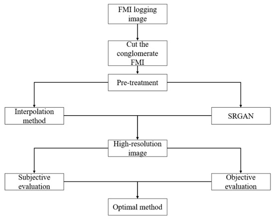
Figure 1.
Technology roadmap.
2.2. The Basic Principle of Interpolation Method
2.2.1. Nearest Neighbor Interpolation Method
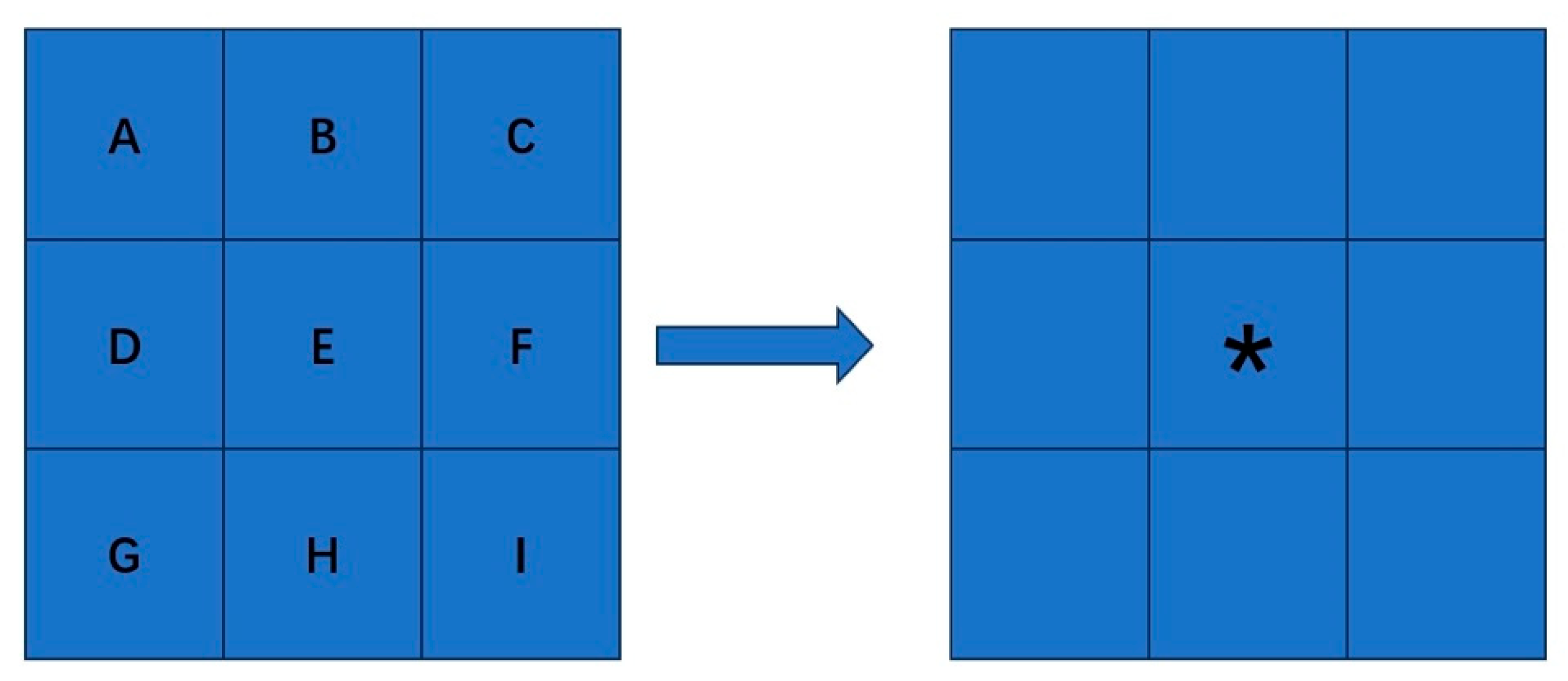
As shown in Figure 2, this method determines the new pixel value based on the minimum geometric distance criterion: After the target pixel (*) is mapped to the original image position, its gray value is directly copied from the nearest spatial neighbor pixel E, and the entire process does not rely on the calculation of surrounding pixels.
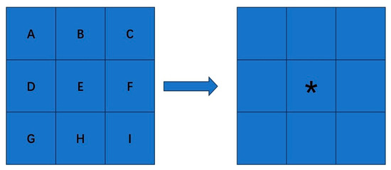
Figure 2.
Schematic diagram of the nearest neighbor interpolation method (“*” represents the target pixel).
This algorithm has the advantage of high computational efficiency, and is suitable for real-time processing systems or scenarios with low complexity (such as icon rendering); however, it will produce significant jagged edges when enlarging images [29], and color gradation discontinuities are prone to occur in the gradual change areas, so it is not suitable for fine texture reconstruction requirements.
2.2.2. Bilinear Interpolation Method
Unlike nearest-neighbor interpolation, which simply copies the nearest pixel, bilinear interpolation performs two linear weighted calculations based on the four neighboring pixels around the target point [30] (Figure 3): first, it linearly interpolates the two pairs of pixels horizontally to obtain the intermediate value, and then it performs a second interpolation on the intermediate value vertically to generate the final pixel, achieving a smooth color transition.
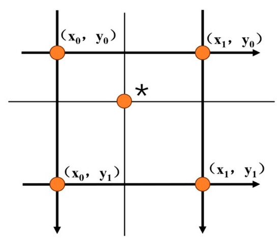
Figure 3.
Schematic diagram of bilinear interpolation method (“*” represents the target pixel).
This method is significantly superior to nearest neighbor interpolation in suppressing the jaggedness and maintaining the smoothness of gradients, and is widely used in scenarios such as image scaling; however, due to the uniform weighted averaging mechanism, it will lose high-frequency details such as textures and sharp edges, resulting in image blurring, especially when magnified at high levels, where the effect significantly deteriorates.
2.2.3. Bicubic Interpolation Method
This method is extended to 16 pixel points within a 4 × 4 neighborhood [30] (Figure 4). After calculating the weights of each pixel using a cubic polynomial function and performing weighted summation, it generates a smoother and clearer image compared to bilinear interpolation. Its higher-order weighting mechanism can produce more smooth and clear images, significantly reducing jaggedness and blurring. It performs exceptionally well in detail and edge reconstruction, but the increased computational complexity leads to a slow processing speed and high memory requirements; moreover, the weight distribution may cause ringing effects (halo-like artifacts) on strong edges, affecting visual quality.
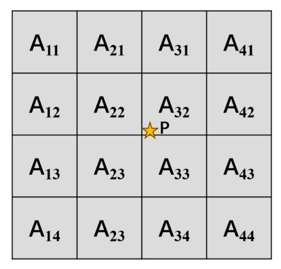
Figure 4.
Schematic diagram of the bicubic interpolation method (The star in figure represents the target pixel).
2.3. The Basic Principles of Generative Adversarial Networks
The Generative Adversarial Network was first proposed by Ian J. Goodfellow et al. in the article ‘Generative Adversarial Nets’ [31] in 2014. Its theoretical framework is based on the zero-sum game and minimax optimization principles in game theory. It achieves data modeling by constructing a dynamic confrontation between the generator and the discriminator. The GAN’s structure is shown in Figure 5. The dynamic confrontation between the generator and the discriminator realizes the modeling of data distribution, and the optimization process is defined by the objective function and converges to the Nash equilibrium. The two follow the objective function as follows:
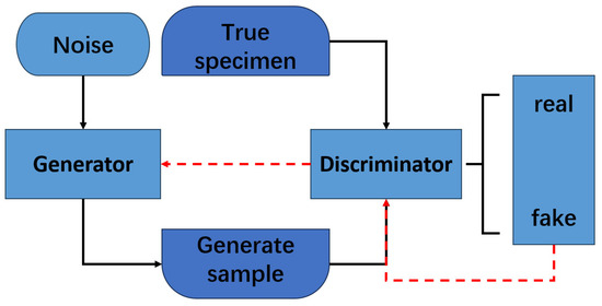
Figure 5.
Schematic diagram of the generative adversarial network structure.
In the formula, represents the real data sample, is the random noise vector, is the sample of the generator, and is the probability that the discriminator determines whether sample is a true sample. are real data samples and follow the real data distribution ; are random noise vectors, following the prior distribution , which is usually a low-dimensional Gaussian distribution or a uniform distribution.
Using alternating training strategies, the generator gradually improves the generation quality until the discriminator is unable to effectively distinguish authenticity (Nash equilibrium state). As a model of unsupervised learning, the GAN can achieve complex distributed modeling without labeled data. Its innovation lies in the adversarial drive mechanism and implicit feature learning ability, and it is widely used in fields such as image synthesis, cross-modal transformation, and data augmentation.
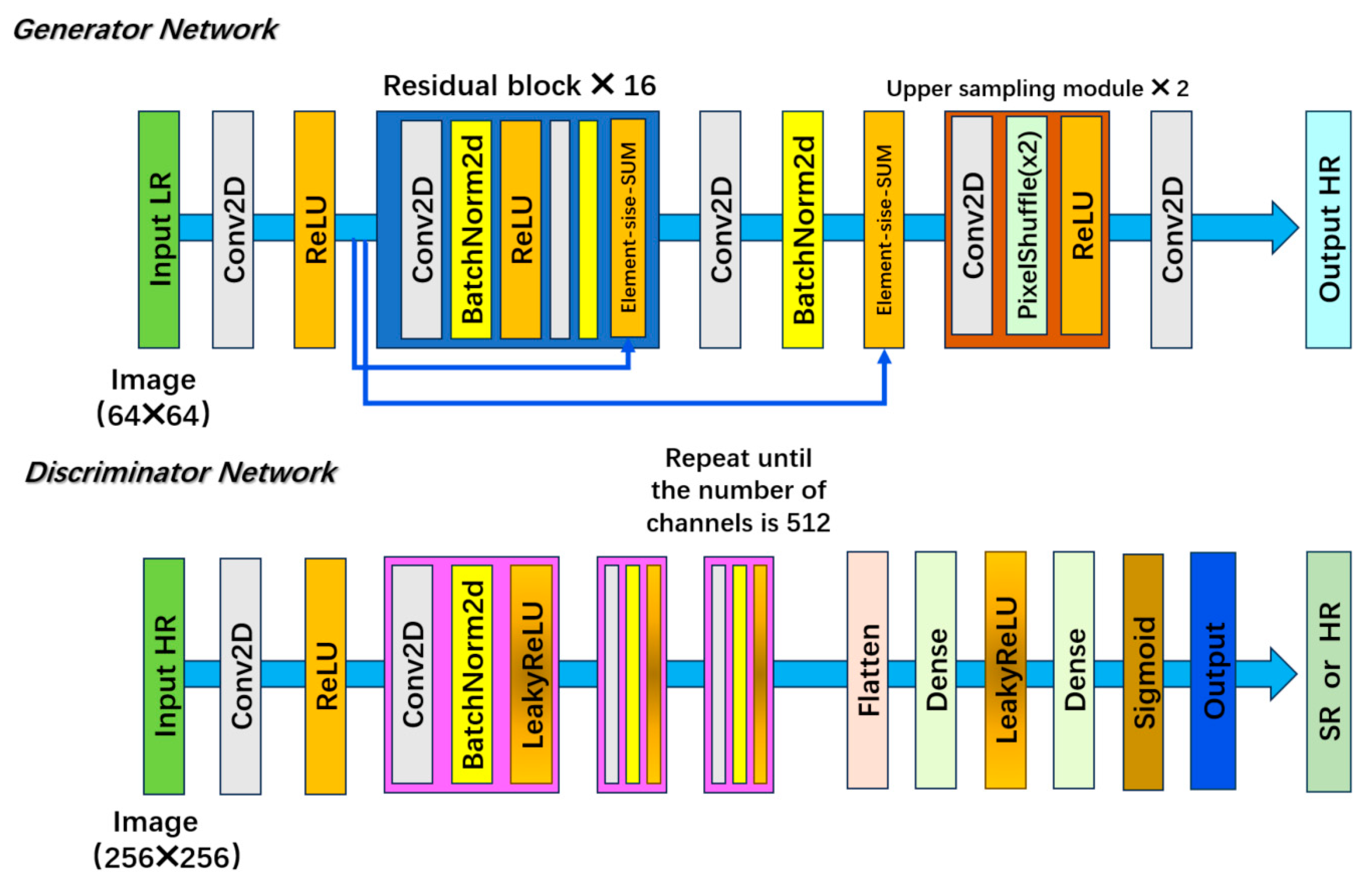
The Super-Resolution Generative Adversarial Network (SRGAN) (Ledig et al., 2017 [16]) breaks through the limitations of traditional pixel-level optimization. Its deep residual generator alleviates the gradient disappearance through residual blocks, achieving the mapping from low resolution to high resolution; the convolutional discriminator drives the adversarial training, forcing the generator to reconstruct high-fidelity texture details, significantly improving the image perception quality. The schematic diagram of its structure is shown in Figure 6.
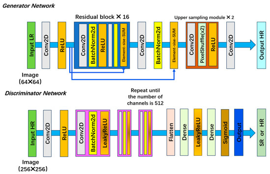
Figure 6.
Schematic diagram of the structure of super-resolution generative adversarial networks.
2.4. Evaluation Index
2.4.1. Mean Square Error (MSE)
Mean Squared Error (MSE) is a common indicator for measuring the differences between two sets of data (Such as the predicted value and the actual value, or two images). It quantifies the overall deviation by calculating the mean squared of the differences between data points, and is widely used in fields such as regression model evaluation and image quality analysis. The closer the MSE value approaches zero, the more similar the reconstructed image is to the original image. Its calculation formula is
In the formula, is the true value, is the predicted value, and is the total number of data points.
2.4.2. Peak Signal-to-Noise Ratio (PSNR)
Peak Signal-to-Noise Ratio (PSNR) is a detection parameter based on a statistical basis, which is used to evaluate the distortion degree of the processed signal compared to the original signal. It first calculates the Mean Square Error (MSE) between the original signal and the processed signal and then combines the maximum possible value of the signal pixel value to measure the ratio of the peak signal power to the noise power in the signal in decibels. The higher the PSNR value is, the smaller the signal distortion and the better the quality [32]. Generally, 30–50 dB is considered to have better image quality. Its advantages are its simple calculation and intuitive understanding. The disadvantages are that it may not be consistent with an observer’s subjective perception and that it is not suitable for complex scenarios. This indicator is widely applied in fields such as image compression, restoration, and video processing, assisting in the evaluation of algorithm performance and signal quality. The calculation formula of PNSR is as follows:
In the formula, represents the maximum possible value of the pixel value (for example, 255 for an 8-bit image); (Mean Square Error) is the square mean of the pixel-by-pixel differences between the original signal and the reconstructed signal; is the original image; is the image to be evaluated; and represents the image size.
2.4.3. Structural Similarity Index (SSIM)
Structural Similarity Index (SSIM), as an advanced measurement index of image similarity, occupies an important position in the field of image processing and analysis. This index comprehensively considers the similarity between images from three dimensions: luminance, contrast, and structure. It does this by constructing the luminance comparison function, contrast comparison function, and structure comparison function, respectively, and organically combining the three to calculate the final SSIM value. Specifically, its value range is between −1 and 1. Compared to traditional indicators, SSIM has significant advantages. On the one hand, it can highly conform to human visual perception and more accurately reflect the subjective judgment of the human eye in regard to image quality. On the other hand, by using the method of calculating local regions and taking the average value, the local structural changes in the image can be effectively captured. Its calculation formula is the following [33]:
Among them, Equation (5) represents the brightness comparison, Equation (6) represents the contrast comparison, and Equation (7) represents the structure comparison. In the formula, and represent the mean pixel values (luminance) of images and ; and are the standard deviations (contrast) of images and ; represents the covariance (structural correlation) of the two images; and , , and are constants, which are used to avoid a denominator of zero and are usually taken as smaller values. , , are weight parameters and are usually set to 1.
3. Image Preprocessing
3.1. Dataset Preprocessing
In the task of image super-resolution, preprocessing is a key link to optimize the performance of the model. This study adopts preprocessing operations such as grayscale and binarization, aiming to achieve dual goals through data dimension reduction and feature enhancement: on the one hand, it reduces the computational complexity and minimizes the interference of redundant information on the model; on the other hand, the algorithm’s perception ability of image structure is enhanced by highlighting key features. The core of preprocessing lies in suppressing the influence of low-value information (such as illumination noise and chromaticity shift) on the reconstruction process, while selectively retaining the details strongly related to the super-resolution target.
3.1.1. Image Grayscale Processing
FMI logging image are usually composed of red, green, and blue color channels, forming RGB color images. In deep learning tasks, processing RGB images requires a significant amount of time for learning. To improve the learning efficiency, a common practice is to convert three-dimensional RGB images into two-dimensional grayscale images, thereby significantly reducing the learning time of deep learning models. Grayscale images present the picture in continuous light and dark levels by retaining luminance information and eliminating color data. While maintaining the overall luminance distribution and local contrast, they significantly enhance the recognition efficiency of key visual features such as contours and textures.
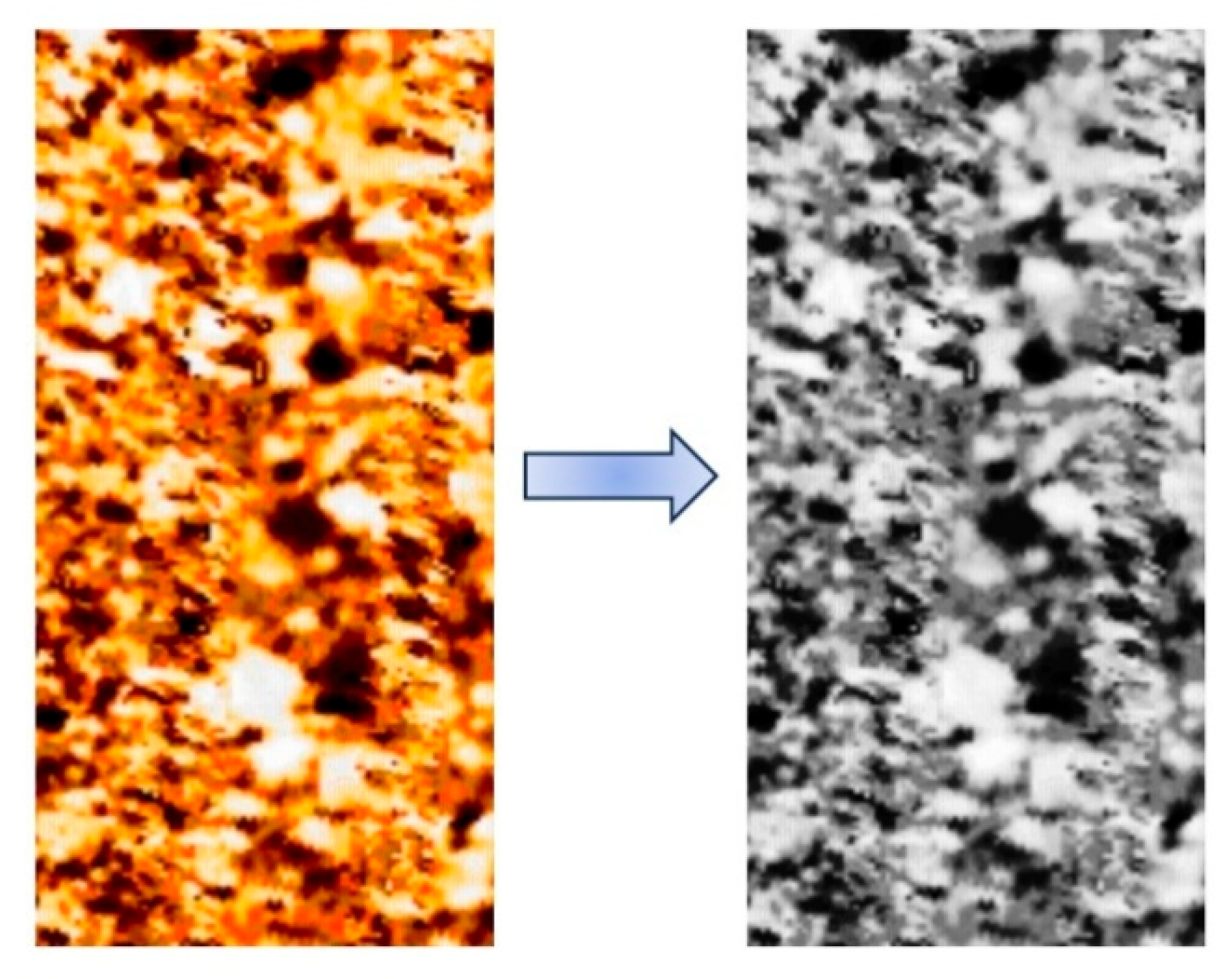
This paper adopts the weighted average value method for grayscale processing. This method generates grayscale images by calculating the weighted average value of the red, blue, and green components of each pixel. The weights can be adjusted as needed to smooth the image while ensuring the image’s detail. Its expression is shown in Equation (9). The grayscale image processed by this algorithm is shown in Figure 7.

Figure 7.
Grayscale processed FMI.
In the formula, is a color image, is a grayscale image, and .
3.1.2. Image Binarization Processing
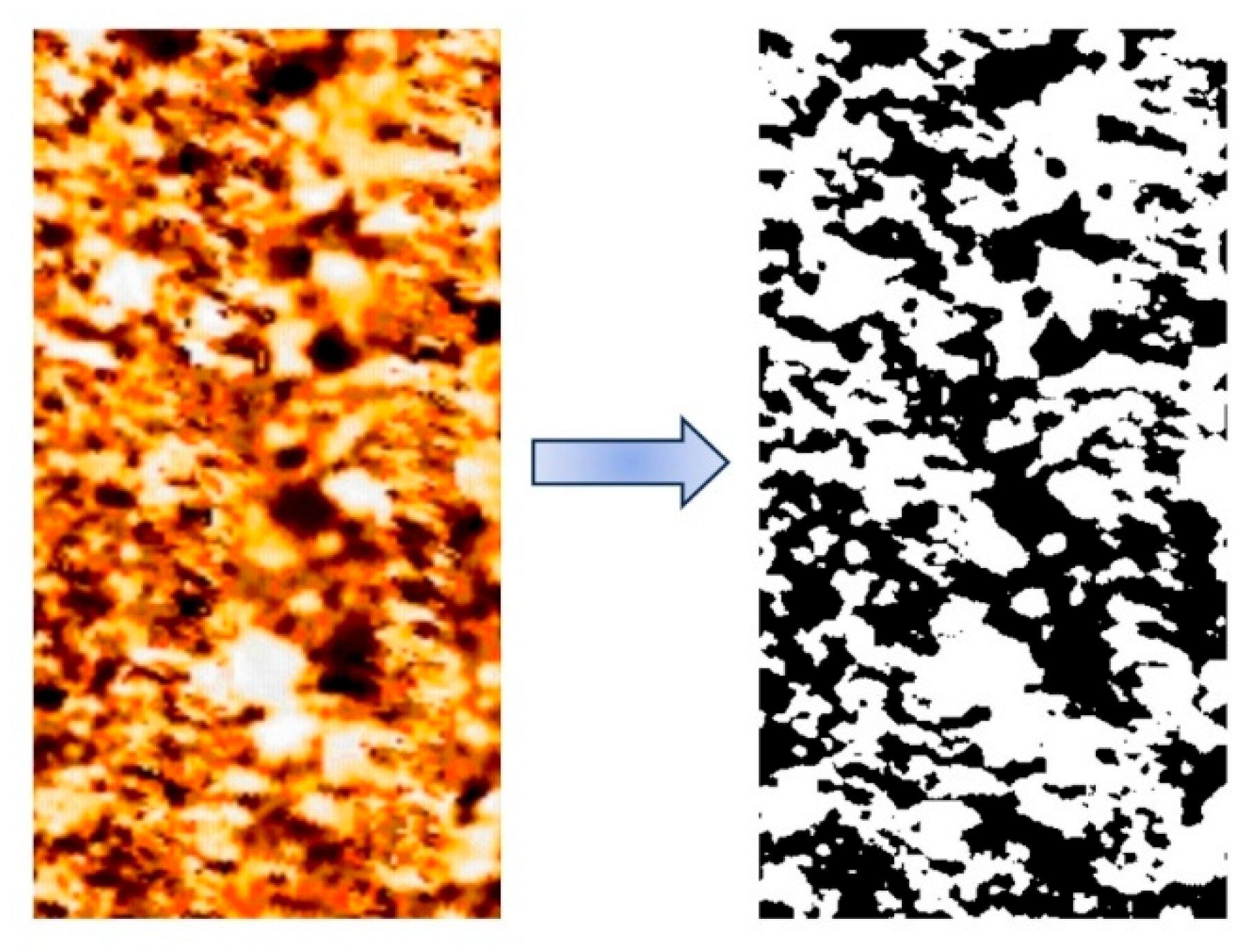
Image binarization is a key technology in digital image processing. Its core lies in converting the gray values of each pixel point in the image into two extreme values, 0 and 255, to present a distinct black and white visual effect of the image. It can ingeniously transform the grayscale image that originally had 256 different brightness levels into an image containing only two grayscale levels, while retaining the overall and local features of the image as much as possible.
Binarization processing techniques are classified into three types: global, local, and adaptive. This paper adopts adaptive binarization. This method can automatically adjust the threshold according to the local characteristics of the image and better preserve the image’s details. The grayscale image processed by this algorithm is shown in Figure 8.
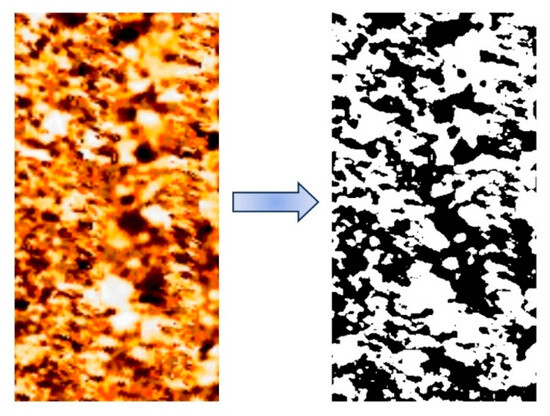
Figure 8.
Binarized FMI.
3.1.3. Training Dataset
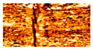
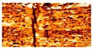
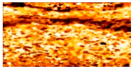
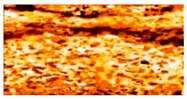
The model needs to be trained in advance before performing super-resolution processing on the image using the SRGAN method. This paper selects the FMI logging image collected from a well in Xinjiang for cropping as the training set. A total of 4855 FMI logging images of conglomerate were cropped in the image library for this training. The rocks in this area are complex and diverse, mainly including conglomerate, unequal-grained small conglomerate, gravel-bearing coarse sandstone, and sandstone. In addition, there are also some mudstones. There are obvious differences in rock structure. There are cases with poor sorting ability and roundness, as well as types of gravel with certain roundness and sorting ability. The cementing material is mainly composed of clayey and calcareous substances. Its color shows a gradual change from bottom to top, gradually changing from mainly brown and dark brown to mainly grayish green and gray. This color transition clearly reveals the evolution process of the sedimentary environment from the fan delta plain to the leading edge of the fan delta, which is a typical manifestation of the sedimentary characteristics of the aquifer period.
The Baikouquan Formation reservoir in the Mabei Slope area is mainly composed of gray and grayish green conglomerate, sandy conglomerate, and sandstone with uneven grain sizes, presenting a unique and diverse geological landscape. The size of gravel varies greatly. The diameter of the largest gravel can reach 10 cm, while the diameters of the commonly distributed gravel are mostly between 0.5 and 2 cm. The morphology of these pebbles is mostly subangular, reflecting that they have undergone a certain degree of weathering and wear. The cementation degree of the reservoir is within the range of medium to dense, and it has good structural stability and permeability.
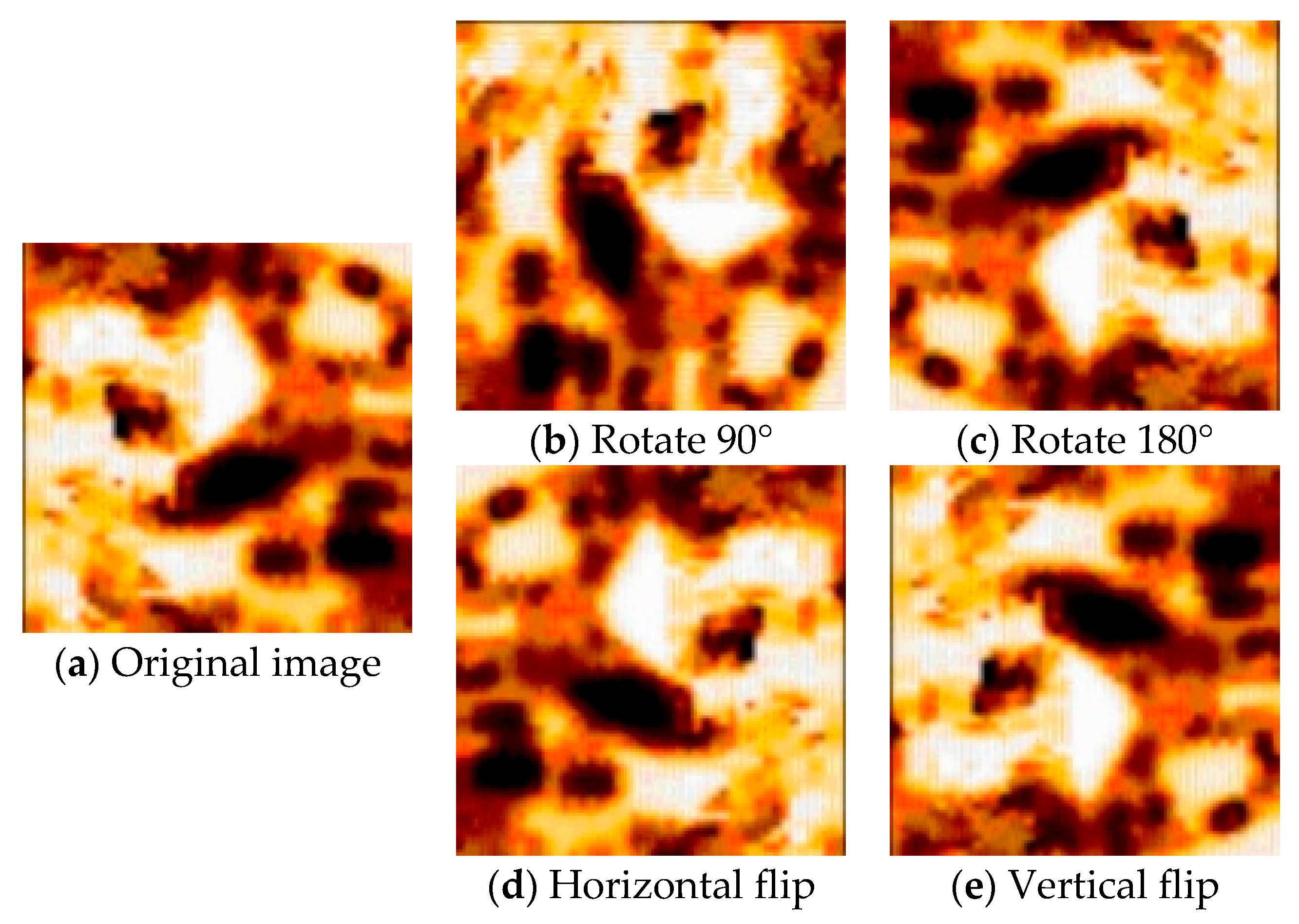
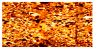
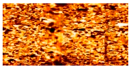
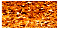
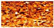
Before the model training begins, 40 images that meet the requirements are first extracted from a whole logging FMI and cropped to a resolution of 128 × 128. Then, operations such as rotating 90°, rotating 180°, horizontal flipping, and vertical flipping are performed on the cropped image set to expand the data diversity and quantity, as shown in Figure 9. The purpose of this operation is to avoid the problem of overfitting caused by the relatively single materials in the database during the model training process [34]. By implementing the above operations, not only was the database expanded to 24,275 images, but also the model’s ability to recognize image changes was enhanced, improving its performance in practical applications.

Figure 9.
Training dataset.
3.2. Training Process
This paper uses an Intel(R) Xeon(R) w7-3465X CPU as the processor of the equipment, with a main frequency of 2.50 GHz and 256 G of memory. The graphics card is NVIDIA GeForce RTX4090 (The GPU was designed by NVIDIA of the United States, while these motherboards were assembled by Dell of the United States as the manufacturer. The production facility is located in the Dell cooperative factory in Xiamen, China). During the training iterations, the batch size is set to 256, and 1000 iterations are conducted. The relevant parameters are shown in Table 2, Table 3, Table 4 and Table 5. This paper sets the program to save once every 25 rounds. After 1000 iterations, a total of 40 sets of models were saved to select the optimal model.
Table 2.
Generator model parameter table.
Table 3.
Discriminator model parameter table.
Table 4.
Optimizer parameters.
Table 5.
Loss function configuration table.
Based on the specified hardware platform (NVIDIA RTX 4090 GPU, 256 GB RAM), the time taken to complete the RGB image calculation task with 25 training rounds ranges from 30 to 35 min. When extended to 1000 iterations, the total computing time is expected to be approximately 22 h. When extended to grayscale images and binary images, the total computing time is effectively reduced by 40–60 min.
3.2.1. RGB Training Model
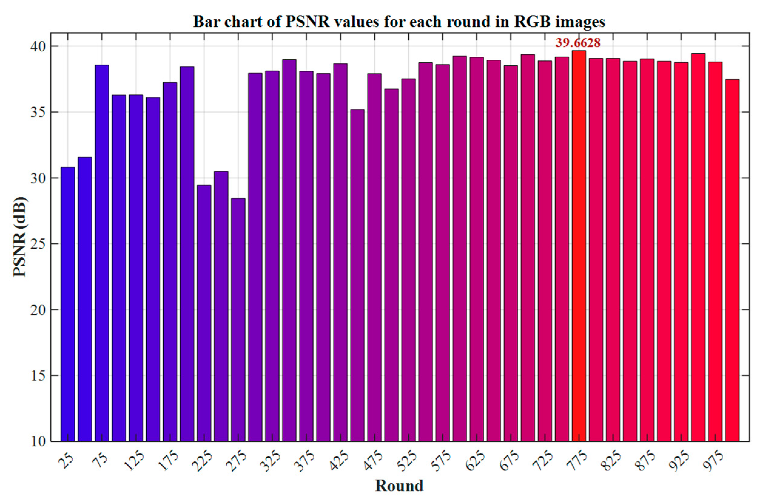
In view of the limitations of subjective evaluation methods in determining the optimal model (such as strong subjectivity and the lack of unified quantitative standards), this paper selects Peak Signal-to-Noise Ratio (PSNR) as the objective evaluation index of RGB image quality to scientifically quantify the model’s performance. Although PSNR is less sensitive to structural distortion and chromaticity deviation [35,36], its strong adaptability to noise types and data distribution, as well as its strong correlation with MSE, still make it a key reference index in the early stage of algorithm development or in tasks dominated by linear noise [37]. In conclusion, PSNR provides a reliable benchmark for the model evaluation in this paper in terms of balancing efficiency, objectivity, and engineering practicality. The comparison indicators of each round are shown in Figure 10 below.

Figure 10.
Bar chart of PSNR values for each round in RGB images.
As shown in Figure 10, the model reaches the maximum value of the Peak Signal-to-Noise Ratio (PSNR) at the 775th training round, indicating that its pixel-level fidelity capability for RGB images has reached the optimal state. Therefore, this paper will select the model of this round as the benchmark model for RGB image testing to ensure that the evaluation results are strictly aligned with the theoretical optimal performance.
3.2.2. Grayscale Training Mode
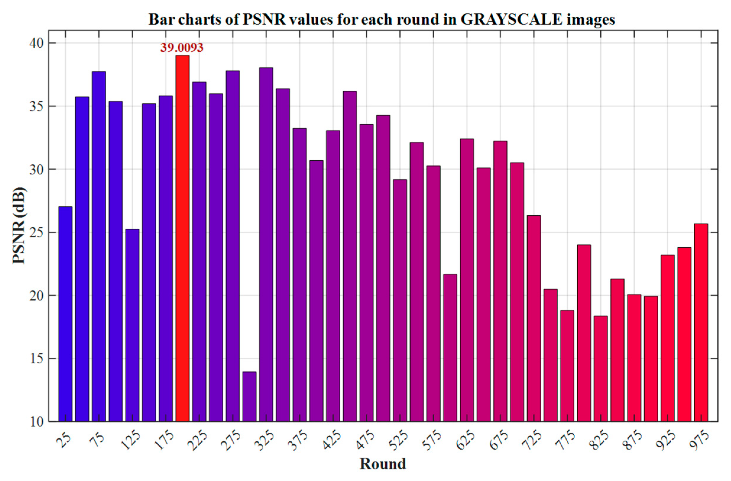
PSNR is applicable to the quality assessment of grayscale images. Its calculation, based on the Mean Square Error of pixels, can effectively quantify luminance distortion (such as Gaussian noise and compression artifacts) [36], and achieve cross-image comparison through dynamic range normalization. Although it is not sensitive to structural distortions such as edge blurring, its high efficiency and strong correlation with errors still make it a core indicator in pixel-level fidelity tasks such as denoising and compression.
As shown in Figure 11, the model reaches the maximum value of the Peak Signal-to-Noise Ratio (PSNR) at 200 training rounds, indicating that the pixel-level fidelity of the grayscale image is optimal at this stage. Therefore, this paper selects this round of model as the benchmark model for grayscale testing to ensure the consistency between the evaluation results and the theoretical performance.

Figure 11.
Bar chart of PSNR values for each round in grayscale images.
3.2.3. Binary Training Model
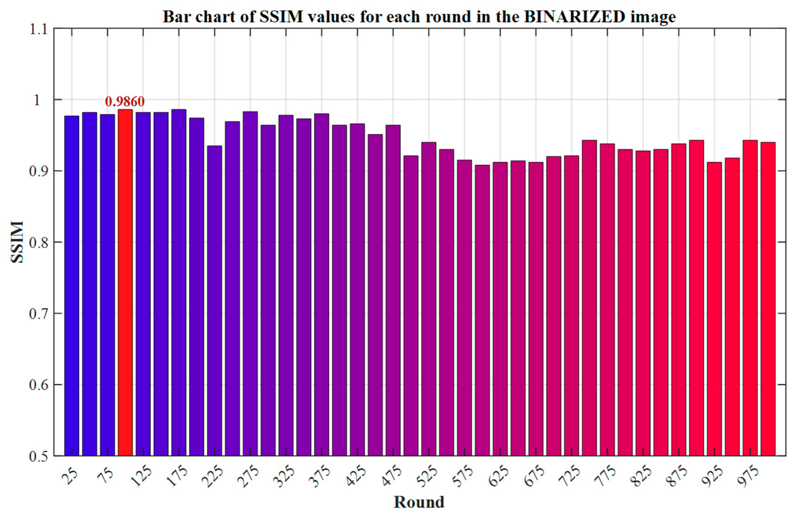
In image quality assessment, PSNR is not applicable to binarized images because it only relies on pixel-level error calculation. However, pixels in binary images only have two states: black and white. A single misjudgment can cause significant fluctuations in the PSNR, but such minor errors have a limited impact on human vision. On the contrary, the SSIM can be used for evaluations by analyzing the overall structure of the image (such as its shape, contour, and relative position). Even if there are local pixel errors, as long as the key structure is retained, it can still objectively reflect the visual quality [37,38], and is more suitable for the evaluation requirements of binary images. The evaluation values of the SSIM in each round are shown in Figure 12 below.
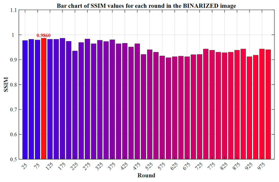
Figure 12.
Bar chart of SSIM values for each round in the binarized image.
As shown in Figure 12, the model achieves the peak of the Structural Similarity Index (SSIM) at the 100th training round, indicating that its retention ability for key structural features of binarized images, such as edge continuity and shape integrity, has reached the optimum. Therefore, this paper selects this round of model as the benchmark model for binarization testing to ensure that the evaluation results are strictly aligned with the structural fidelity objective.
3.3. Binary Training Model
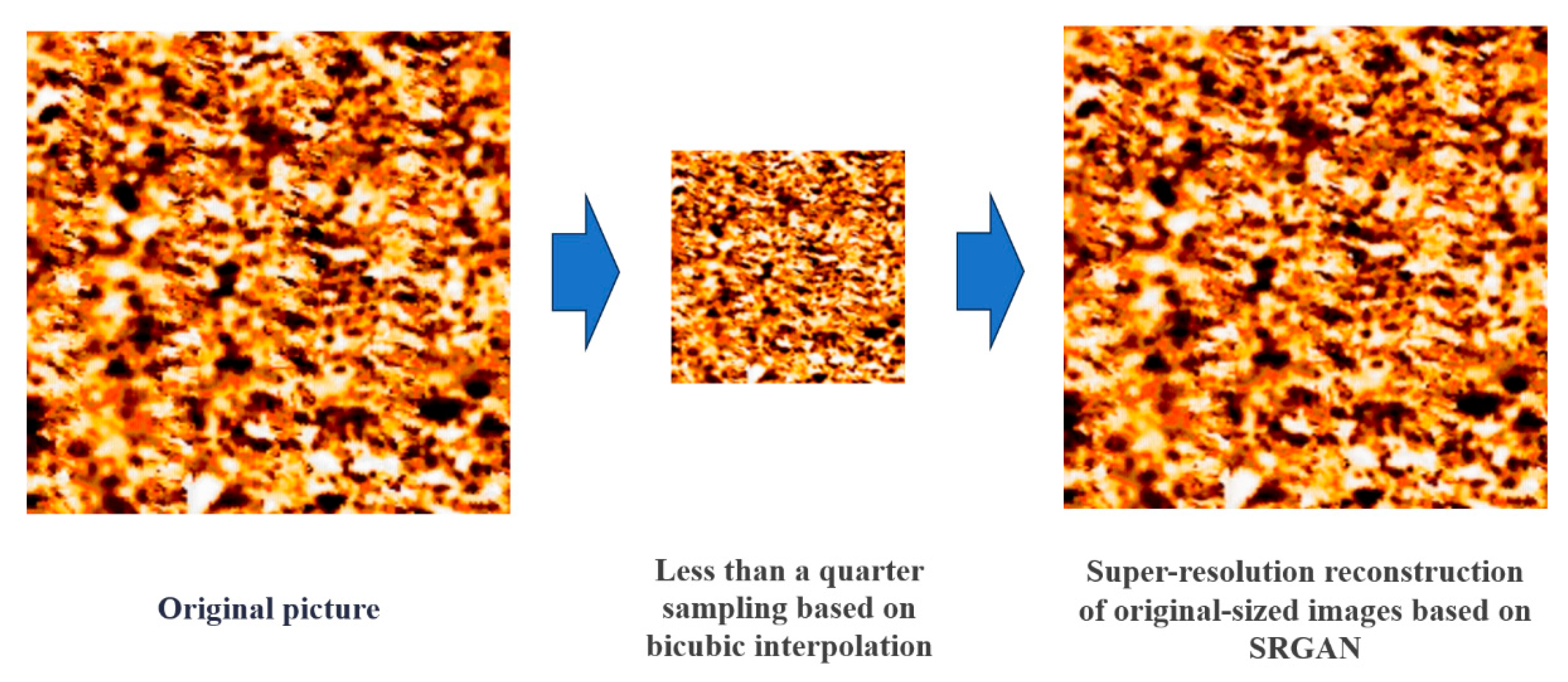
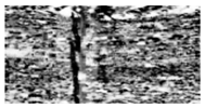
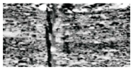
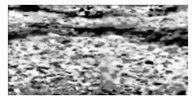
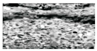
As shown in Figure 13, to verify the authenticity of FMI logging image, this study adopts the degradation and reconstruction processes to detect potential tampering traces. In the specific process, the original 512 × 512-pixel RGB-FMI is downsampled using bicubic interpolation to generate 128 × 128 low-resolution samples, simulating the image degradation process. The pre-trained SRGAN model is used to perform super-resolution reconstruction on the downsampled samples and restore their resolution to the original size. Through visual comparison and structural similarity analysis (SSIM = 0.9116), it was found that the reconstructed image has a high degree of consistency with the original image in terms of texture details and edge continuity.
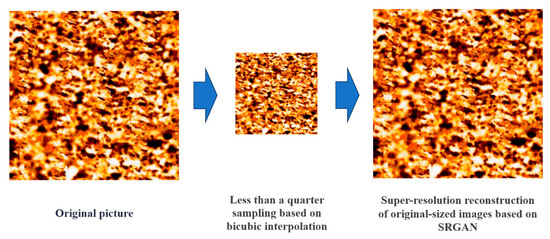
Figure 13.
Comparison chart of feature consistency between the reconstructed image of SRGAN and the original sample.
4. Training Results and Analysis
4.1. Analysis of RGB Image Results
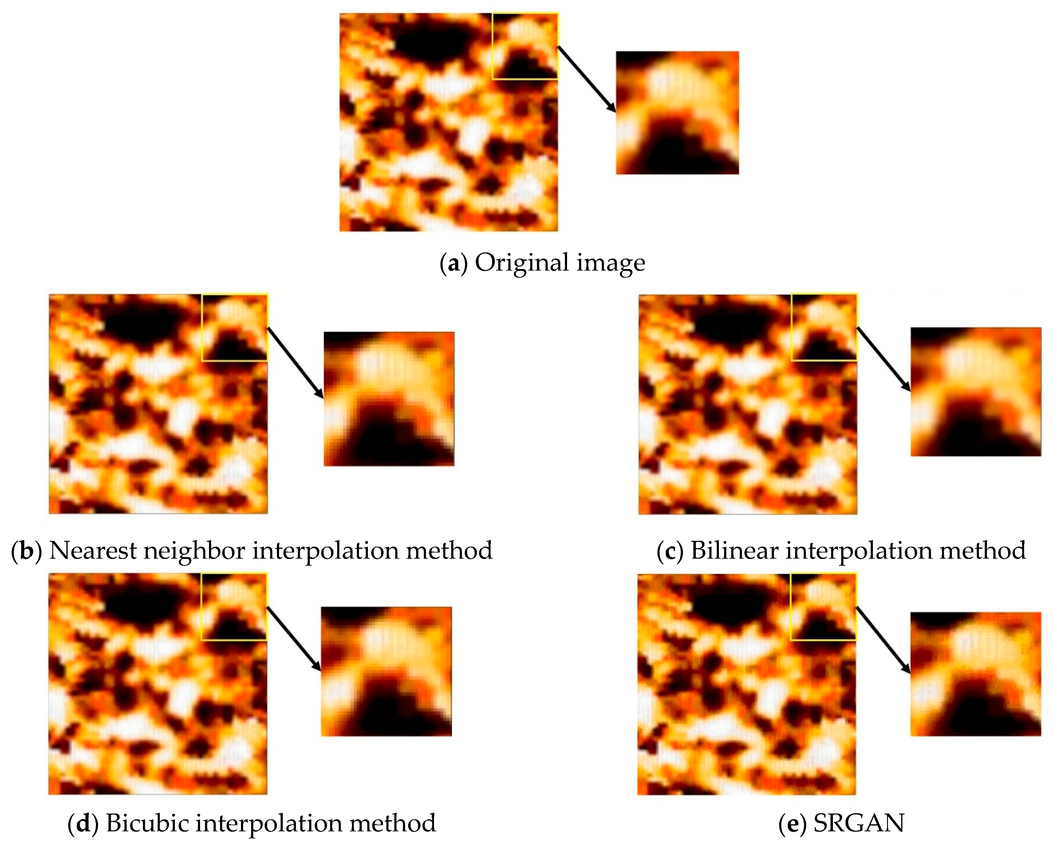
As shown in Figure 14, in terms of the overall reconstruction effect, the bicubic interpolation method, among the traditional interpolation methods, performs the worst. The edges of the images it generates have obvious jagged and mosaic phenomena, accompanied by color distortion problems. In contrast, the bilinear interpolation method performs better among various interpolation algorithms. Although it can avoid the mosaic effect caused by the nearest neighbor interpolation method, there are still blurring problems at the edge details. The SRGAN algorithm, on the other hand, demonstrates significant advantages. It not only completely eliminates edge aliasing and mosaic phenomena, but also significantly outperforms the bilinear interpolation method in terms of detail clarity. Furthermore, this method effectively suppresses color distortion and artifact generation, achieving an image reconstruction effect which has higher accuracy and is closer to the real scene.

Figure 14.
Comparison of the local RGB effect of a certain image magnified twice in the database.
As can be seen from the quantitative evaluation results in Table 6, whether it is the PSNR index for measuring pixel-level fidelity or the SSIM for evaluating structural consistency and visual perception quality, the SRGAN algorithm is significantly superior to traditional interpolation methods. This result further verifies its superiority in the super-resolution reconstruction task.
Table 6.
Results of RGB image resolution calculation using objective methods.
4.2. Analysis of Grayscale Image Results
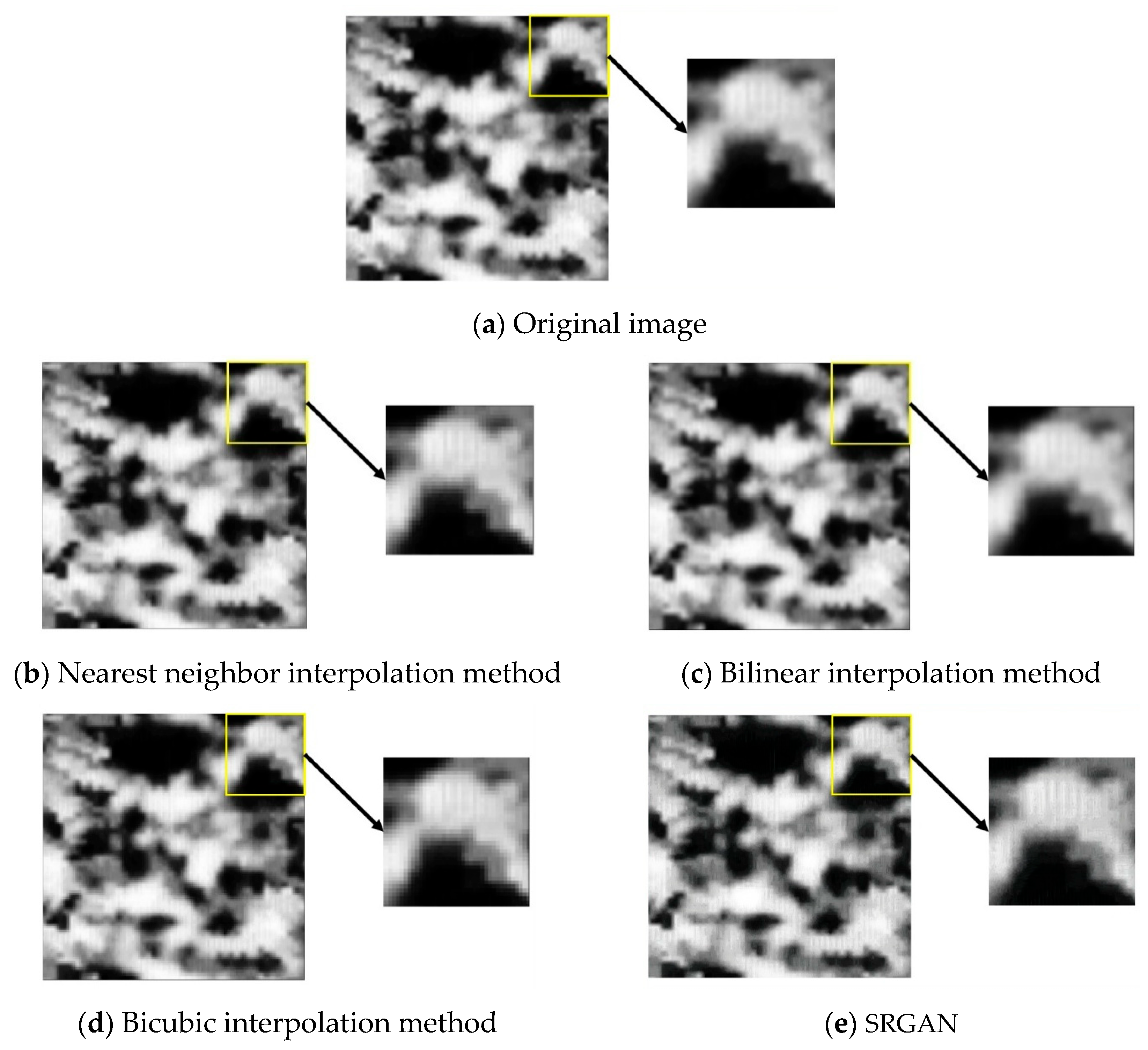
It can be observed from the overall reconstruction effect presented in Figure 15 that, after grayscale processing of the logging FMI, the processed image can still well-reflect the particle size distribution characteristics of the entire image, and, at the same time, it can effectively highlight the contour information of the conglomerate. Grayscale processing not only retains the original particle size information and gravel contour of the image, but also significantly reduces the computational complexity and greatly improves the computational efficiency by simplifying the three-channel gradient calculation of the RGB image to a single-channel calculation. In the application of image interpolation methods, the effects of both the nearest neighbor interpolation method and the bicubic interpolation method are not ideal. The specific manifestations are as follows: After processing using the nearest neighbor interpolation method, obvious mosaic phenomena occur when the image is locally magnified, and the contour serration is severe. Although the bicubic interpolation method alleviates the jagged problem, there is still the situation of edge blurring. In contrast, although the bilinear interpolation method avoids the mosaic phenomenon, the overall image clarity is insufficient, and the contour edges are still not sharp enough after local magnification. Using comparative experiments, it was found that the SRGAN algorithm performed the best in grayscale image processing. Compared to RGB images, grayscale processing effectively eliminates the problems of edge blurring and defocusing caused by local highlights, thereby significantly improving the quality of the magnified image. This improvement enables grayscale images to maintain better clarity and edge sharpness after magnification.
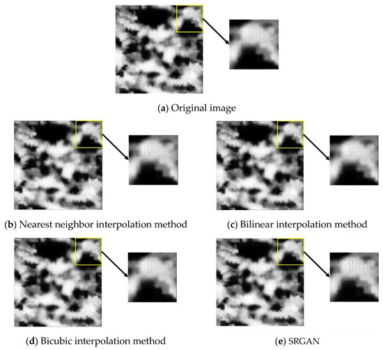
Figure 15.
Comparison of the local grayscale effect of a certain image magnified twice in the database.
The data analysis in Table 7 shows that, compared to RGB images, the quality of the grayscale processed images slightly improved when reconstructed using the interpolation method. Under the evaluation of the two indicators of PSNR and SSIM, the SRGAN method based on deep learning performs the best, and its reconstruction effect is significantly better than that of the traditional interpolation algorithm. This indicates that SRGAN can better restore image details, especially with obvious advantages when dealing with edges and textures.
Table 7.
The resolution results of grayscale images are calculated by objective methods.
4.3. Analysis of BINARY Image Results
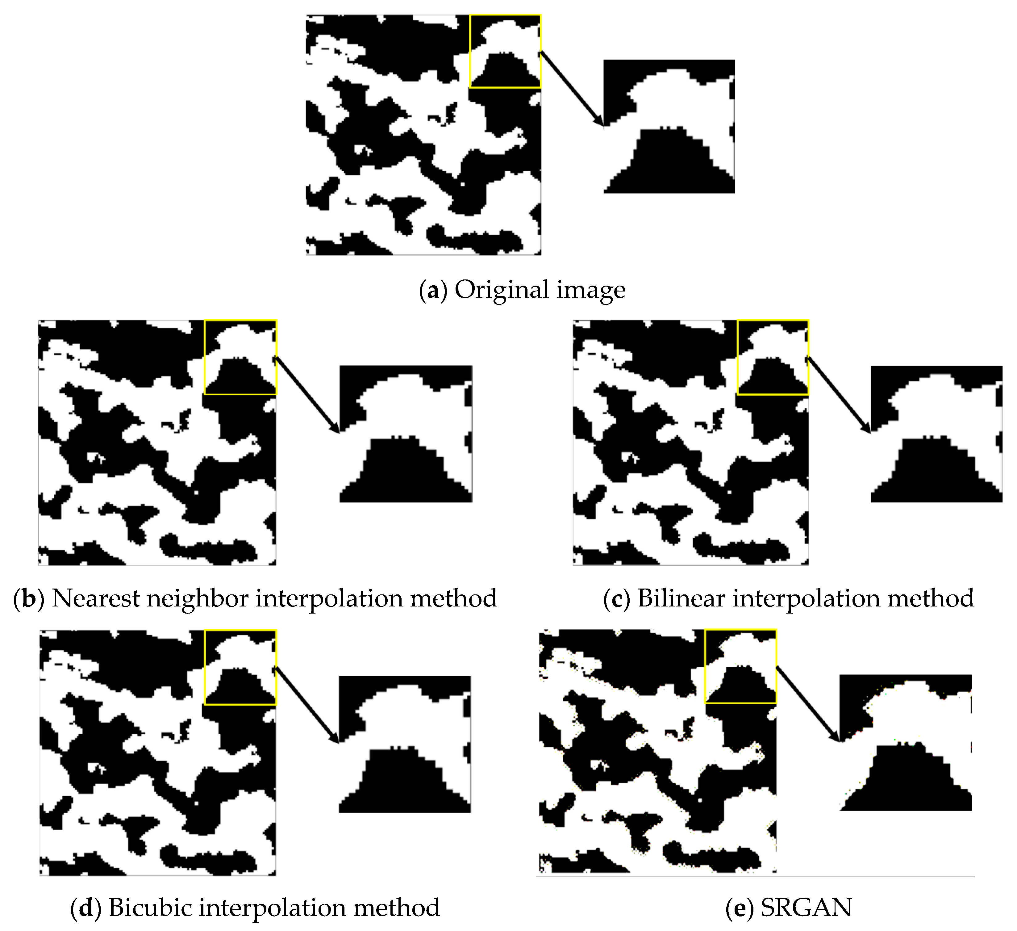
Judging from the overall reconstruction effect of each binarized image in Figure 16, the entire image presents both black and white colors. By comparing the grayscale image in Figure 15, it can be observed that, during the process of converting the grayscale image to binary, data loss occurs in some areas. When performing interpolation reconstruction and SRGAN super-resolution reconstruction, only the contour of the conglomerate can be made as smooth as possible, and the ideal gravel diameter and porosity cannot be observed.
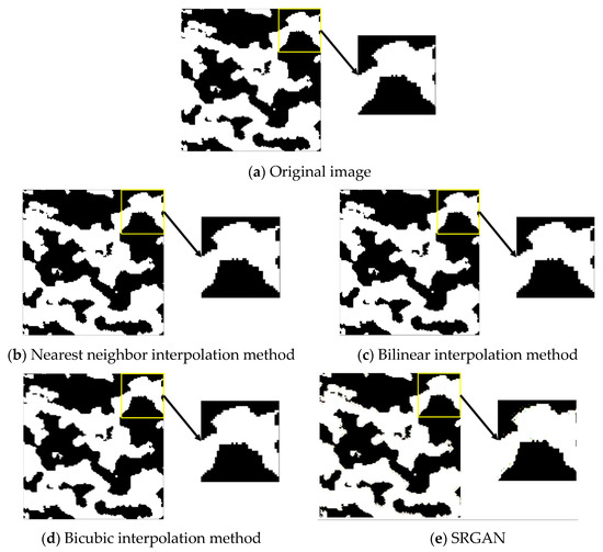
Figure 16.
Comparison of the local BINARY effect of a certain image magnified twice in the database.
It can be observed in Table 8 that, when comparing interpolation methods, SRGAN still shows a relatively superior reconstruction effect. However, when comparing color logging FMI logging image, whether subjectively or objectively, the superiority of SRGAN over conventional interpolation methods is not particularly prominent.
Table 8.
Results of BINARY image resolution calculation by objective methods.
4.4. Image Tests in Other Wells
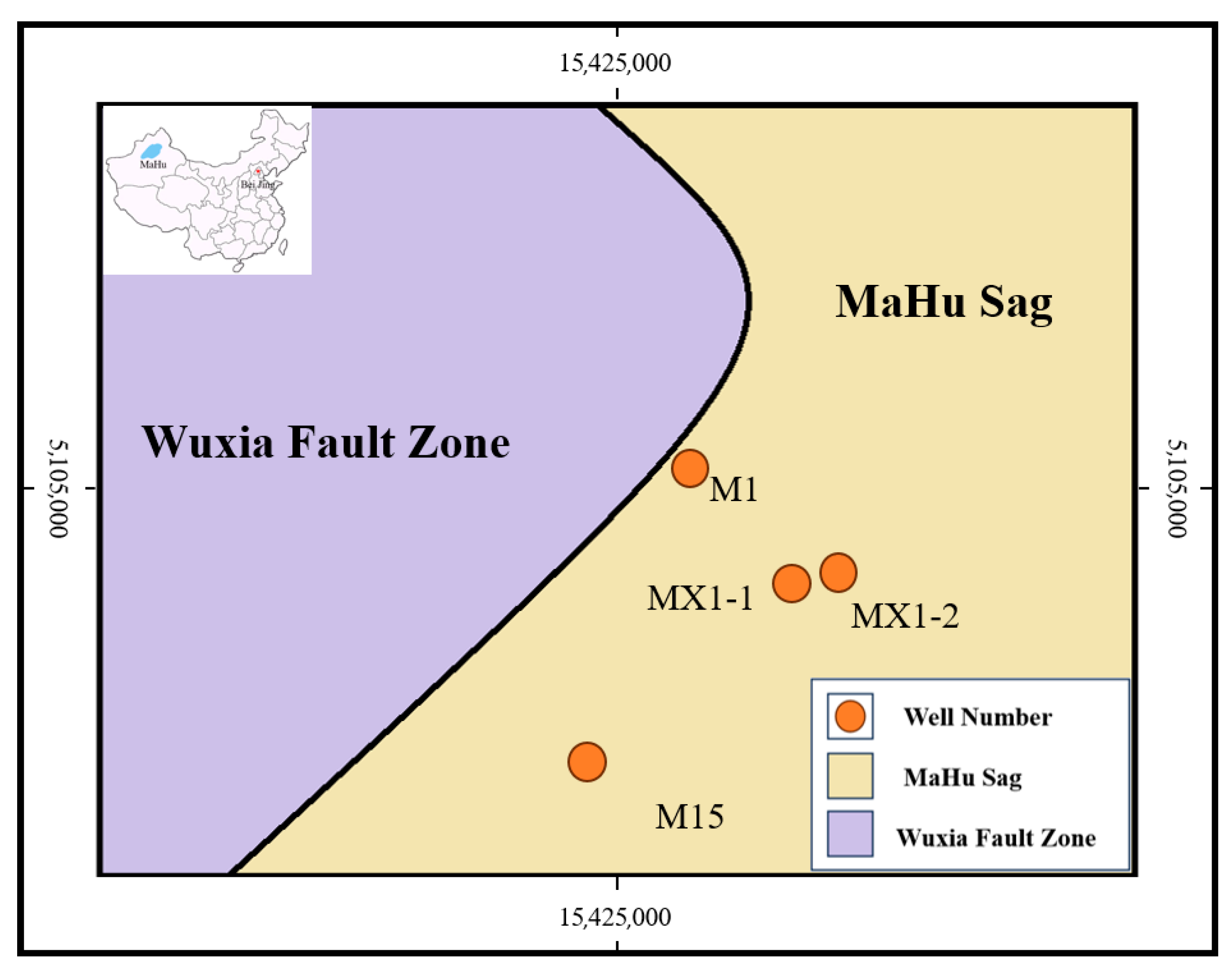
To comprehensively evaluate the generalization performance of the model, this study selected FMI logging image from four different drilling wells in the Mahe Oilfield, namely M1, MX1-1, MX1-2, and X93, to form an independent test set. Their location distribution is shown in Figure 17. These well positions cover diverse geological conditions and wellbore environments, aiming to effectively verify the model’s adaptability to unseen data.

Figure 17.
Geological map of the well locations in the northern part of Mahu Lake.
The test results (Table 9, Table 10 and Table 11) show that the key indicators (PSNR, SSIM) remained stable on the data of the four wells, indicating that the model has good robustness. Importantly, the super-resolution results can clearly present the key geological features at different well positions: the fracture structure of M1 well, the lithologic stratification boundary of MX1-1 well, and the smaller sand-gravel body boundaries in MX1-2 and X93 wells.
Table 9.
Comparison and evaluation table of RGB images in other wells.
Table 10.
Comparison and evaluation table of grayscale images in other wells.
Table 11.
Comparison and evaluation table of BINARY images in other wells.
5. Discussion
To reveal the microstructure of gravel rock layers more clearly, this paper adopts the image super-resolution method to carry out super-resolution reconstruction of logging FMI logging image of gravel rock. Firstly, the logging FMI logging image were subjected to grayscale and binarization processing successively. Then, three different interpolation methods, namely the nearest neighbor interpolation method, bilinear interpolation method, and bicubic interpolation method, as well as the deep learning SGANR method, were, respectively, applied to implement super-resolution processing on the logging FMI logging image of three different colors.
To determine the optimal method for improving the quality of logging FMI logging image, two evaluation methods were adopted: one is subjective evaluation, through which the edge, contour, and other information of the processed high-resolution images are observed by the human eye; the second is objective evaluation, with the aid of computer mathematical models to calculate image quality.
As shown in Table 12, based on the comparison of experimental data, SRGAN demonstrates significant advantages in the super-resolution tasks of RGB, grayscale, and binary images. Among the traditional interpolation methods, bilinear interpolation performed better in RGB (0.740) and grayscale images (0.901), but SRGAN improved by 34.0% and 9.9%, respectively. Bicubic interpolation works best in binary images (0.837), but SRGAN still achieves a performance improvement of 17.2%. Although traditional interpolation methods still have application value in scenarios with limited real-time performance or computing resources, SRGAN, with its precise restoration ability of texture and structure, has become a better choice for high-precision super-resolution tasks.
Table 12.
Performance comparison table between traditional interpolation methods and SRGAN.
This study adopts the SRGAN algorithm based on deep learning, aiming to improve the quality of FMI logging image with the help of this algorithm. Previous studies have shown that, when using SRGAN super-resolution dense sandstone images [24], the PSNR increases by more than 20 dB, which is lower than the optimal value (41.39 dB) in this paper. However, in terms of SSIM, it is consistent with this paper.
This study chose SRGAN over more advanced models like ESRGAN, mainly based on the following three considerations:
- Core objective compatibility: As the first study to introduce GAN into the field of FMI super-resolution, it is necessary to first verify the basic feasibility. The SRGAN structure is simple and the training is stable, which is more conducive to the preliminary verification of cross-domain technology transfer.
- Computational efficiency and data size: The complex structure of ESRGAN (such as the RRDB module) requires higher computational resources and data volume. However, this study is limited by the professional FMI dataset size, and the lightweight design of SRGAN can reduce the risk of overfitting.
- Geological feature fidelity requirements: The enhanced natural image textures of ESRGAN may interfere with the geometric structure of rock layer fractures (such as introducing artifacts), while SRGAN retains the structural foundation through the VGG content loss, which is more in line with the geological interpretation requirements.
Table 13 summarizes the current research status of SRGAN in some fields. By comparing and analyzing the research goals, methods, problems solved, and limitations of different teams, the deficiencies of the existing technology are clarified. At the same time, the table highlights the innovative positioning of this study—introducing SRGAN (Super-Resolution Generative Adversarial Network) into FMI super-resolution reconstruction, aiming to solve the core bottlenecks, such as the low resolution of FMI logging image, that are preventing subsequent work from being carried out, and providing a more accurate data foundation for reservoir characterization.
Table 13.
Comparison table of SRGAN-related research.
Table 13 systematically summarizes the applications of SRGAN and its variants in various fields such as digital elevation models, rock CT imaging, satellite remote sensing, UAV haze removal, and medical images for super-resolution tasks. Comparative analysis reveals that their common advantages lie in significantly enhancing images’ high-frequency details through adversarial training and perceptual loss, with PSNR/SSIM indicators generally superior to traditional methods (such as bicubic interpolation); however, current research focuses on natural scenes and general objects, and has not yet covered FMI super-resolution in geological exploration, and the pre-processing strategies mostly target color or noise, lacking optimization for geological structural features. Therefore, this study applies SRGAN to FMI reconstruction, innovatively combining grayscale/binarization pre-processing to adapt to geological features, achieving a significant performance breakthrough with PSNR 41.39 dB/SSIM 0.992, which is far superior to similar studies (such as SSIM 0.906 for rock CT and PSNR 29.93 dB for satellite images). This not only fills the gap in SRGAN’s application in petroleum geological image super-resolution, but also highlights the innovative nature of its structured pre-processing scheme and cross-domain performance advantages; more importantly, this study has solved the core bottleneck of the insufficient resolution of FMI logging image restricting geological analysis, providing a high-precision data basis for crack identification and reservoir modeling, and having significant engineering application value.
It should be noted that this study does not systematically compare the potential advantages of other super-resolution methods on FMI logging image. This requires subsequent verification through extensive code implementation and rigorous experiments. Therefore, it is currently impossible to assert whether there exists a better alternative to the method (SRGAN combined with grayscale/binarization preprocessing) presented in this paper. In future work, we will conduct a more comprehensive comparative study on this issue.
This study conducted the super-resolution task on a workstation equipped with an NVIDIA RTX 4090 GPU and 256 GB RAM. However, considering that this hardware may not be widely available in practical applications, a workstation equipped with an NVIDIA RTX A4000 GPU (256 GB RAM) was also used for the comparative experiment. The results show that the processing time of the RTX A4000 was approximately twice that of the RTX 4090. Given that the peak FP32 computing power of the RTX A4000 is approximately 38.7 TFLOPS while that of the RTX 4090 is about 82.6 TFLOPS, the computing power gap between the two is approximately 2.13 times. This result is in good agreement with the measured time increase. Therefore, subsequent studies can estimate the approximate running time by combining the computing power parameters of the target hardware. Additionally, if the RAM configuration is reduced, the batch processing size can be appropriately decreased to maintain program operation, but this will correspondingly prolong the calculation time.
The binarization process (such as converting electrical imaging grayscale/RGB images into lithology boundaries or fracture maps) irreversibly loses crucial continuous gray gradient information (such as the sharpness of gravel edges, internal fine textures, and precise transitions of pore morphology). This results in highly sparse generated binary image information, with an extremely simple structure (mainly sharp boundaries), and an extremely low information entropy. The advantages of perceptual-driven super-resolution models like SRGAN lie in restoring or generating complex textures that conform to natural statistical laws. Their perceptual loss and adversarial training mechanisms heavily rely on the rich structure and gray gradient information contained in the input data. However, the binary input lacks the original data foundation required for reconstructing fine geological structures, and its extremely simple nature also makes the goal of “enhancing visual naturalness” both unnecessary and difficult to achieve. The model finds it challenging to learn effective structural information beyond basic boundary smoothing from such limited information.
Therefore, whether it is traditional interpolation (which can achieve higher pixel accuracy, but with limited improvement) or SRGAN, when dealing with binary input, they are unable to restore the fine structure and original grayscale texture information that determine key quantitative geological analysis indicators such as grain size, porosity, and crack opening degree. Their main effect is limited to optimizing the appearance of the boundary (smoothing/anti-aliasing), which is insufficient and may even be misleading for geological interpretation, which requires sub-pixel accuracy and original gradient details. The fundamental solution is as follows: super-resolution processing must be performed on the original grayscale or RGB image. Only by retaining the complete continuous grayscale information can a rich data foundation be provided for deep learning models to reconstruct the fine geological features (edges, textures, shapes) at a high resolution, ensuring the accuracy of subsequent quantitative geological analysis.
The core innovation of this study lies in pioneering the application of the Super-Resolution Generative Adversarial Network (SRGAN) technology specifically to address the critical bottleneck issue of insufficient resolution in full wellbore micro-resistivity scanning imaging (FMI) logging images. This problem directly restricts its performance in core geological application scenarios, such as the precise analysis of rock grain size and accurate identification of rock types. The driving force behind this innovative application does not stem from the technology itself, but rather from the urgent needs of actual geological research: when using conventional FMI logging image for key tasks such as filling in blind area information, precise rock type discrimination, and quantitative extraction of grain size, the inherent resolution limitations of these images result in blurred image details and unclear boundaries, seriously affecting the accuracy and reliability of the subsequent analysis. Faced with the dilemma that traditional image-enhancement methods cannot meet the precision requirements of geological interpretation, we first explored, and successfully verified, the powerful effectiveness of SRGAN in significantly improving the resolution of geological FMI logging image, thereby significantly enhancing the execution effect of downstream geological tasks and providing an innovative and efficient solution to this long-standing practical problem that has long concerned geologists.
The deep learning model proposed in this study effectively enhances the visual clarity of the geological boundaries of sandstone and gravel in logging FMI logging image. Through an adaptive sharpening mechanism, it significantly suppresses the edge blurring caused by downhole noise and instrument limitations. Theoretical analysis confirms that this technology can enhance the edge representation of key geological features such as lithology interfaces, rock structures, and dissolution cavities. However, it must be pointed out that the model has inherent scale-sensitivity limitations: due to the limitations of the original image resolution and the algorithm’s perception ability, its reconstruction effect on sub-pixel-level fine geological structures (such as extremely fine-grained gravel and micro-fracture systems) is limited, and, in strong heterogeneous regions, it may cause local over-smoothing effects due to the loss of high-frequency information. These boundaries are essentially constrained by the synergy of data acquisition capabilities and model architecture. In the future, it is necessary to break through the current technical threshold by using multi-source data fusion and cross-scale modeling.
This research’s findings have broad application prospects. In the field of oil and gas field development, the images reconstructed in super-resolution can help engineers identify reservoir characteristics more accurately, optimize well location deployment, improve the efficiency of oil and gas extraction, and reduce extraction costs. In terms of geological feature assessment, clear images help geologists analyze information, such as stratum structure and the sedimentary environment, more accurately, providing a reliable basis for geological disaster prediction and resource exploration, and facilitating the more scientific and reasonable development and utilization of Earth’s resources.
6. Conclusions
In this paper, the logging FMI logging image are made grayscale and binarized. The resolutions of the logging FMI logging image of sandstone and gravel are improved by using the interpolation method and the SRGAN method. The results calculated using the interpolation method and the SRGAN method are compared using the comprehensive visual quality assessment and the quantitative index analysis of PSNR, SSIM, and MSE, and the following conclusions are obtained:
- (1)
- Using data analysis, the image representation form and algorithm characteristics jointly affect the super-resolution reconstruction effect: In the traditional interpolation method, the grayscale image achieves the optimal balance (PSNR 29.39/SSIM 0.901) through bilinear interpolation, and its SSIM value is increased by 21.7% compared with the same method in the RGB domain; however, SRGAN shows significant advantages in the RGB domain. With the indicators of PSNR 41.39 and SSIM 0.992, it far exceeds the best interpolation algorithm (bicubic interpolation: PSNR increased by 61.6%, SSIM increased by 34.1%).
- (2)
- The above data indicate that SRGAN demonstrates the optimal boundary reconstruction ability in RGB, grayscale, and binary images: In the RGB domain, it shows significant superiority with a PSNR of 41.39 (an increase of 61.6% compared to the best interpolation method by two or three times) and an SSIM of 0.992 (an increase of 49.3%). In the grayscale domain, its PSNR of 40.15 and SSIM of 0.99 still maintain an advantage, increasing by 36.6% and 9.9%, respectively, compared to bilinear interpolation. This stable performance across modalities verifies the algorithmic advantages of SRGAN in FMI boundary restoration.
- (3)
- Although the binary images achieved the lowest MSE (1353.66) and the highest SSIM (0.981) in SRGAN, the structural details of the gravel could not be effectively reconstructed due to the absence of the color dimension, revealing the decoupling phenomenon between the objective evaluation indicators and the characterization ability of geological features.
- (4)
- The effect of generative adversarial neural networks in improving image resolution is superior to that of traditional interpolation methods, indicating that the feasibility of using computer deep learning methods to improve the resolution of FMI logging images of conglomerate is high. In the field of image enhancement algorithms, traditional interpolation methods have limited resolution improvement when dealing with complex logging FMI logging image of conglomerate. However, generative adversarial neural networks can learn image features through adversarial training and generate high-quality and high-resolution images with broad prospects. In oil and gas exploration, high-precision FMI logging image are very crucial. Deep learning methods can meet the requirements, provide better solutions, and facilitate scientific decision-making and efficient exploration.
Author Contributions
Conceptualization, C.M., X.Q. and J.F.; software, C.M.; validation, X.Q. and Z.L.; writing—original draft preparation, C.M.; writing—review and editing, X.Q.; formal analysis, C.M.; resources, L.C. and Y.L.; project administration, Y.L.; data curation, L.C.; visualization, Z.L.; supervision, J.F. All authors have read and agreed to the published version of the manuscript.
Funding
This study was financially supported by the Open Project of Key Laboratory of Green Mining of Coal Resources of Ministry of Education in Xinjiang; the project number is KLXGY-Z2409.
Data Availability Statement
Data are contained within the article.
Conflicts of Interest
Authors Liangyu Chen and Yonggui Li were employed by China National Logging Corporation. The remaining authors declare that the research was conducted in the absence of any commercial or financial relationships that could be construed as a potential conflict of interest.
References
- Jiu, K.; Ding, W.; Huang, W.; Zhang, Y.; Zhao, S.; Hu, L. Fractures of lacustrine shale reservoirs, the Zhanhua Depression in the Bohai Bay Basin, eastern China. Mar. Pet. Geol. 2013, 48, 113–123. [Google Scholar] [CrossRef]
- Wang, Z.; Xiang, H.; Wang, L.; Xie, L.; Zhang, Z.; Gao, L.; Yan, Z.; Li, F. Fracture Characteristics and its Role in Bedrock Reservoirs in the Kunbei Fault Terrace Belt of Qaidam Basin, China. Front. Earth Sci. 2022, 10, 865534. [Google Scholar] [CrossRef]
- Sun, S.; Huang, S.; Gomez-Rivas, E.; Griera, A.; Liu, B.; Xu, L.; Wen, Y.; Dong, D.; Shi, Z.; Chang, Y.; et al. Characterization of natural fractures in deep-marine shales: A case study of the Wufeng and Longmaxi shale in the Luzhou Block Sichuan Basin, China. Front. Earth Sci. 2022, 17, 337–350. [Google Scholar] [CrossRef]
- Yin, S.; Tian, T.; Wu, Z. Developmental characteristics and distribution law of fractures in a tight sandstone reservoir in a low-amplitude tectonic zone, eastern Ordos Basin, China. Geol. J. 2020, 55, 17. [Google Scholar] [CrossRef]
- He, B.; Liu, Y.; Qiu, C.; Liu, Y.; Su, C.; Tang, Q.; Tian, W.; Wu, G. The Strike-Slip Fault Effects on the Ediacaran Carbonate Tight Reservoirs in the Central Sichuan Basin, China. Energies 2023, 16, 4041. [Google Scholar] [CrossRef]
- Bei, W.; Xiangjun, L.; Liqiang, S.I.M.A. Grading evaluation and prediction of fracture-cavity reservoirs in Cambrian Longwangmiao Formation of Moxi area, Sichuan Basin, SW China. Pet. Explor. Dev. 2019, 46, 301–313. [Google Scholar] [CrossRef]
- Ren, Y.; Wei, W.; Zhu, P.; Zhang, X.; Chen, K.; Liu, Y. Characteristics, classification and KNN-based evaluation of paleokarst carbonate reservoirs: A case study of Feixianguan Formation in northeastern Sichuan Basin, China. Energy Geosci. 2023, 4, 100156. [Google Scholar] [CrossRef]
- Gao, L.; Shi, X.; Liu, J.; Chen, X. Simulation-based three-dimensional model of wellbore stability in fractured formation using discrete element method based on formation microscanner image: A case study of Tarim Basin, China. J. Nat. Gas Sci. Eng. 2022, 97, 104341. [Google Scholar] [CrossRef]
- Pang, H.; Chen, M.; Wang, H.; Jin, Y.; Lu, Y.; Li, J. Lost circulation pattern in the vug-fractured limestone formation. Energy Rep. 2023, 9, 941–954. [Google Scholar] [CrossRef]
- Chen, S. The Wavelet Transformation Sensitiveness to Direction of Image Characteristics and its Application in Formation MicroScanner Image Fracture Identification. Sens. Transducers J. 2014, 173, 16. [Google Scholar]
- Yu, Z.; Wang, Z.; Wang, J. Continuous Wavelet Transform and Dynamic Time Warping-Based Fine Division and Correlation of Glutenite Sedimentary Cycles. Math. Geosci. 2022, 55, 521–539. [Google Scholar] [CrossRef]
- Xiang, R.; Yang, H.; Yan, Z.; Mohamed Taha, A.M.; Xu, X.; Wu, T. Super-resolution reconstruction of GOSAT CO2 products using bicubic interpolation. Geocarto Int. 2022, 37, 15187–15211. [Google Scholar] [CrossRef]
- Wang, Y.; Rahman, S.S.; Arns, C.H. Super resolution reconstruction of μ-CT image of rock sample using neighbour embedding algorithm. Phys. A 2018, 493, 177–188. [Google Scholar] [CrossRef]
- Dong, C.; Loy, C.C.; He, K.; Tang, X. Image Super-Resolution Using Deep Convolutional Networks. IEEE Trans. Pattern Anal. Mach. Intell. 2016, 38, 295–307. [Google Scholar] [CrossRef] [PubMed]
- Da Wang, Y.; Armstrong, R.T.; Mostaghimi, P. Enhancing Resolution of Digital Rock Images with Super Resolution Convolutional Neural Networks. J. Pet. Sci. Eng. 2019, 182, 106261. [Google Scholar] [CrossRef]
- Ledig, C.; Theis, L.; Huszár, F.; Caballero, J.; Cunningham, A.; Acosta, A.; Aitken, A.; Tejani, A.; Totz, J.; Wang, Z.; et al. Photo-realistic single image super-resolution using a generative adversarial network. In Proceedings of the IEEE Conference on Computer Vision and Pattern Recognition, Honolulu, HI, USA, 21–26 July 2017; pp. 4681–4690. [Google Scholar]
- Deng, X.; Hua, W.; Liu, X.; Chen, S.; Zhang, W.; Duan, J. D-SRCAGAN: DEM Super-resolution Generative Adversarial Network. IEEE Geosci. Remote Sens. Lett. 2022. [Google Scholar] [CrossRef]
- Shan, L.; Liu, C.; Liu, Y.; Kong, W.; Hei, X. Rock CT Image Super-Resolution Using Residual Dual-Channel Attention Generative Adversarial Network. Energies 2022, 15, 5115. [Google Scholar] [CrossRef]
- Soltanmohammadi, R.; Faroughi, S.A. A comparative analysis of super-resolution techniques for enhancing micro-CT images of carbonate rocks. Appl. Comput. Geosci. 2023, 20, 100143. [Google Scholar] [CrossRef]
- Lil, R.; Liu, W.; Gong, W.; Zhu, X.; Wang, X. Super resolution for single satellite image using a generative adversarial network. ISPRS annals of the photogrammetry, remote sensing and spatial information sciences. ISPRS Ann. Photogramm. Remote Sens. Spat. Inf. Sci. 2022, 5, 591–596. [Google Scholar]
- Zhang, T.; Hu, G.; Yang, Y.; Du, Y. A Super-Resolution Reconstruction Method for Shale Based on Generative Adversarial Network. Transp. Porous Media 2023, 150, 383–426. [Google Scholar] [CrossRef]
- Li, J.; Teng, Q.; Zhang, N.; Chen, H.; He, X. Deep learning method of stochastic reconstruction of three-dimensional digital cores from a two-dimensional image. Phys. Rev. E 2023, 107, 055309. [Google Scholar] [CrossRef] [PubMed]
- Zhou, R.; Wu, C. 3D reconstruction of digital rock guided by petrophysical parameters with deep learning. Geoenergy Sci. Eng. 2023, 231, 212320. [Google Scholar] [CrossRef]
- Liu, B.; Chen, J. A super resolution algorithm based on attention mechanism and SRGAN network. IEEE Access 2021, 9, 139138–139145. [Google Scholar] [CrossRef]
- Wang, C.H.; Yan, Y.M.; Han, X.W.; Liang, T.; Wan, Z.; Wang, Q. Dehazing Algorithm for UAV Aerial Images Based on Improved SRGAN. Laser Infrared 2024, 54, 991–997. [Google Scholar]
- Jadhav, P.; Sairam, V.A.; Bhojane, N.; Singh, A.; Gite, S.; Pradhan, B.; Bachute, M.; Alamri, A. Multimodal Gas Detection Using E-Nose and Thermal Images: An Approach Utilizing SRGAN and Sparse Autoencoder. Comput. Mater. Contin. 2025, 83, 3493–3517. [Google Scholar] [CrossRef]
- Sun, C.; Wang, C.; He, C. Image Super-Resolution Reconstruction Algorithm Based on SRGAN and Swin Transformer. Symmetry 2025, 17, 337. [Google Scholar] [CrossRef]
- Güngür, Z.; Ayaz, I.; Tümen, V. Biomedical Image Super-Resolution Using SRGAN: Enhancing Diagnostic Accuracy. BEU Fen Bilim. Derg. 2025, 14, 198–212. [Google Scholar] [CrossRef]
- Wang, F.; Zhao, J. Digital Core Image Reconstruction Based on Deep Learning and Evaluation of Reconstruction Effect. J. Cent. South Univ. (Nat. Sci. Ed.) 2022, 53, 4412–4424. [Google Scholar]
- Xie, H.; Xie, K.; Yang, H. Research Progress of Image Super-resolution Methods. Comput. Eng. Appl. 2020, 56, 34–41. [Google Scholar]
- Goodfellow, I.J.; Pouget-Abadie, J.; Mirza, M.; Xu, B.; Warde-Farley, D.; Ozair, S.; Courville, A.; Bengio, Y. Generative Adversarial Nets. Adv. Neural Inf. Process. Syst. 2020, 27, 2672–2680. [Google Scholar]
- Jia, J. Face Super-Resolution Reconstruction Based on Generative Adversarial Nets and Face Recognition. Master’s Thesis, University of Electronic Science and Technology of China, Chengdu, China, 2018; p. 14. [Google Scholar]
- Zhu, X.; Yao, S.; Sun, B.; Qian, Y. Image quality assessment: Combining the characteristics of HVS and structural similarity index. J. Harbin Inst. Technol. 2018, 50, 121–128. [Google Scholar]
- Li, W.; Zhang, X. Depth Image Super-resolution Reconstruction Method Based on Convolutional Neural Network. J. Electron. Meas. Instrum. 2017, 31, 1918–1928. [Google Scholar]
- Wang, Z.; Bovik, A.C.; Sheikh, H.R.; Simoncelli, E.P. Image quality assessment: From error visibility to structural similarity. IEEE Trans. Image Process. 2004, 13, 600–612. [Google Scholar] [CrossRef] [PubMed]
- Horé, A.; Ziou, D. Image Quality Metrics: PSNR vs. SSIM. In Proceedings of the 2010 20th International Conference on Pattern Recognition, Istanbul, Turkey, 23–26 August 2010; pp. 2366–2369. [Google Scholar]
- Huynh-Thu, Q.; Ghanbari, M. Scope of validity of PSNR in image/video quality assessment. Electron. Lett. 2008, 44, 800–801. [Google Scholar] [CrossRef]
- Zhang, L.; Zhang, L.; Mou, X.; Zhang, D. FSIM: A Feature Similarity Index for Image Quality Assessment. IEEE Trans. Image Process. 2011, 20, 2378–2386. [Google Scholar] [CrossRef] [PubMed]


Disclaimer/Publisher’s Note: The statements, opinions and data contained in all publications are solely those of the individual author(s) and contributor(s) and not of MDPI and/or the editor(s). MDPI and/or the editor(s) disclaim responsibility for any injury to people or property resulting from any ideas, methods, instructions or products referred to in the content. |
© 2025 by the authors. Licensee MDPI, Basel, Switzerland. This article is an open access article distributed under the terms and conditions of the Creative Commons Attribution (CC BY) license (https://creativecommons.org/licenses/by/4.0/).