Investigation on Corrosion-Induced Wall-Thinning Mechanisms in High-Pressure Steam Pipelines Based on Gas–Liquid Two-Phase Flow Characteristics

Abstract

In high-pressure thermal power systems, corrosion-induced wall thinning in steam pipelines poses a significant threat to operational safety and efficiency. This study investigates the effects of gas–liquid two-phase flow on corrosion-induced wall thinning in pipe bends of high-pressure heaters in power plants, with particular emphasis on the mechanisms of void fraction and inner wall surface roughness. Research reveals that an increased void fraction significantly enhances flow turbulence and centrifugal effects, resulting in elevated pressure and Discrete Phase Model (DPM) concentration at the bend, thereby intensifying erosion phenomena. Simultaneously, the turbulence generated by bubble collapse at the bend promotes the accumulation and detachment of corrosion products, maintaining a cyclic process of erosion and corrosion that accelerates wall thinning. Furthermore, the increased surface roughness of the inner bend wall exacerbates the corrosion process. The rough surface alters local flow characteristics, leading to changes in pressure distribution and DPM concentration accumulation points, subsequently accelerating corrosion progression. Energy-Dispersive Spectroscopy (EDS) and Scanning Electron Microscopy (SEM) analyses reveal changes in the chemical composition and microstructural characteristics of corrosion products. The results indicate that the porous structure of oxide films fails to effectively protect against corrosive media, while bubble impact forces damage the oxide films, exposing fresh metal surfaces and further accelerating the corrosion process. Comprehensive analysis demonstrates that the interaction between void fraction and surface roughness significantly intensifies wall thinning, particularly under conditions of high void fraction and high roughness, where pressure and DPM concentration at the bend may reach extreme values, further increasing corrosion risk. Therefore, optimization of void fraction and surface roughness, along with the application of corrosion-resistant materials and surface treatment technologies, should be considered in pipeline design and operation to mitigate corrosion risks.

1. Introduction

With growing energy demands and increasingly stringent environmental protection requirements, the efficient operation and reliability of large-scale thermal power units have become research priorities. In thermal power units, high- and low-pressure heaters utilize steam extraction from turbines to gradually heat boiler feedwater, enhancing heat exchange efficiency [1,2]. However, with steam as the shell-side medium and water as the tube-side medium, the condensation of heating steam in the shell affects heat exchange efficiency through water level variations [3,4]. Excessive water levels submerge heat exchange tubes, preventing effective heat transfer, while insufficient levels can lead to tube bundle overheating and damage from high-temperature steam. Therefore, the reliability of water level control signal tubes is crucial. Field inspections have frequently revealed that signal tube bends and tees often experience wall thinning and leakage, leading to unplanned shutdowns or emergency heater isolation, severely impacting normal operations [5,6].

Gas–liquid two-phase flow is prevalent in chemical engineering, nuclear power, cryogenic engineering, and oil–gas transportation [7,8]. In practical applications, pipeline transport typically involves flow channels in different directions, necessitating the use of bent pipes, with 90° bends being the most common. Compared to single-phase flow, two-phase flow introduces liquid buoyancy, creating complex flow characteristics when passing through 90° bends due to the combined effects of gravity, centrifugal force, and buoyancy. These effects can generate flow reversal, overflow, and secondary flow phenomena, potentially threatening pipeline integrity [9,10].

Current research on gas–liquid two-phase flow in pipelines primarily focuses on experimental and numerical simulation approaches. Huang, Xin et al. studied gas–liquid two-phase flow characteristics in fractured reservoir microcrack networks, particularly examining the liquid properties’ effects on gas flow patterns. They simplified microcrack networks into T-type and Y-type structures, using the Open FOAM software for simulation and experimental validation. The results showed that T-type and Y-type models effectively reproduced two-phase flow characteristics, with volume-of-fluid-model-based symmetry-breaking solutions showing energetic advantages. Liquid phase properties significantly influenced gas flow patterns, while two-phase flow velocity and fluid parameters jointly determined gas flow stability [11]. Wei, Na developed a general transient gas–liquid two-phase wellbore flow model and computational program for numerical simulation. The model, based on phase mass conservation and mixture momentum conservation equations, incorporated phase interactions through the Shi Slip relationship and employed classical MUSCL technology with second-order AUSMV formatting for numerical solutions. The simulation results aligned well with findings in the literature using first-order flux-limited Roe formatting and refined meshes, successfully capturing transient-phase behavior during normal gas kick events [12]. Guo, Wei proposed a thermal diffusion-based flow measurement method for gas–liquid two-phase flow, monitoring wall temperature to capture Taylor bubble and liquid slug velocities and lengths, deriving liquid film thickness. They found linear relationships between the temperature curve average descent slope, liquid slug velocity, and void fraction, establishing a new flow calculation model. Experimental testing showed average relative errors of 3.45% and 5.51% for gas and liquid phase flow predictions, respectively [13]. Xie, Chuan experimentally investigated downhole choke behavior in vertical and horizontal pipes. Testing 40 data points (4 mm choke) and 350 data points (2, 4, 8, and 12 mm chokes), they analyzed flow patterns, pressure, and mass flow rates. The results showed downhole chokes modified downstream flow patterns, enhanced stability, and prevented liquid backflow. Taitel correlations accurately predicted slug–churn flow transition boundaries, while Ashford, Sachdeva, and Al-Safran models achieved the highest prediction accuracy under critical flow conditions [14]. Sha, W numerically investigated inlet void fraction and pipe arrangement effects on oil–gas two-phase flow characteristics in 90° bends. This research showed large-scale vortices with high void fractions formed at inlet void ratios of 0.05–0.15 in both horizontal and vertical arrangements, intensifying oil–gas separation and causing additional head loss. Maximum pressure drops occurred approximately one diameter downstream of bend outlets, initially increasing and then stabilizing with increasing inlet void ratios [15]. Chen, D numerically studied vortex flowmeter applications in the natural gas industry, particularly gas–liquid two-phase flow characteristics. Using RNG K-ε turbulence and Eulerian multiphase flow models for CFD simulation, validated against experimental data, the results demonstrated the effective simulation of two-phase flow characteristics, especially in precession frequency comparisons [16]. Ma et al. used multiphase CFD to model discrete bubble flow in porous granular media and revealed strong local turbulence effects due to bubble breakup, which supports the relevance of void fraction-driven instabilities observed in pipe bends [17].

However, existing studies have rarely focused on the synergistic impact of void fraction and surface roughness on erosion–corrosion coupling in pipe bends, nor have they integrated CFD simulation with microstructural and compositional analysis to uncover the underlying thinning mechanisms. To understand the erosion mechanisms of two-phase flow in non-uniform wall thinning, this study combines experimental and numerical simulation methods to analyze flow evolution characteristics through 90° bends. Using Scanning Electron Microscopy (SEM) imaging, we observed the microscopic structures of pipe inner wall corrosion sections and surfaces, revealing microscopic damage from two-phase flow erosion. Computational Fluid Dynamics (CFD) simulations analyzed pressure distribution and DPM characteristic changes under varying void fractions and bend surface roughness conditions. This combined experimental–numerical approach comprehensively reveals the erosion mechanisms of gas–liquid two-phase flow in non-uniform wall thinning, providing theoretical support for considering fluid dynamics characteristics and material fatigue in system design and operation to reduce erosion and extend pipeline service life. To facilitate clarity, the remainder of this paper is structured as follows: Section 2 presents the experimental and numerical methodologies; Section 3 discusses the results and analysis; and Section 4 concludes with the key findings and implications.

2. Methodology

2.1. Experimental Detection

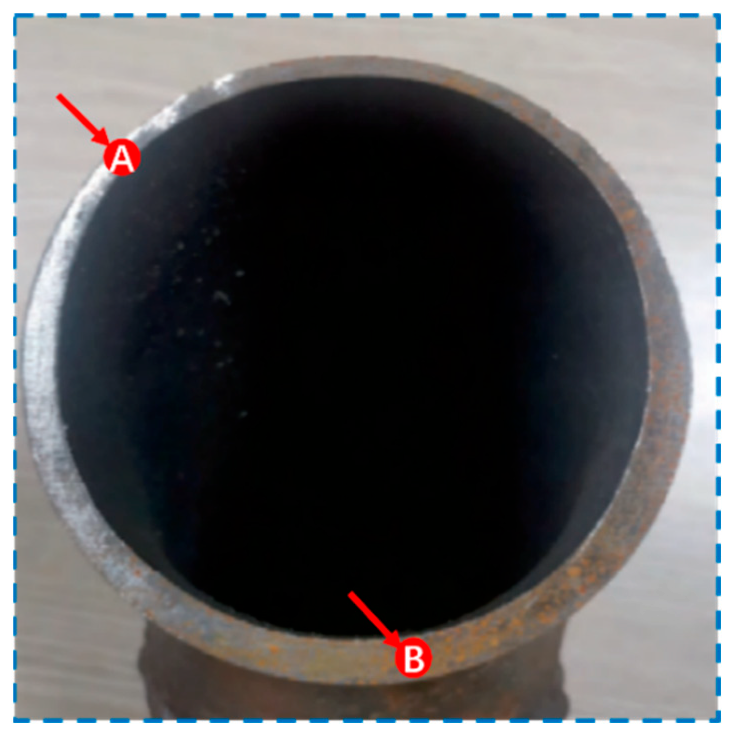
2.1.1. Introduction to In-Service Pipe Bends

This study examines in-service signal tube bends, which, along with tees, are widely used in thermal power units. However, wall-thinning problems frequently occur, resulting in leakage incidents that lead to unplanned shutdowns or emergency heater isolation, severely disrupting normal production processes. The selected bends and tees are made from common industrial pipeline materials with typical microstructures and mechanical properties. Taking a high-pressure heater’s gas–liquid two-phase flow signal tube as an example, significant wall thinning can be observed in the bend section. The basic specifications of this pipeline are as follows: outer diameter of φ89 mm, wall thickness of 5 mm, and material of 20# steel. The working medium is water on the tube side and steam on the shell side, with an operating pressure of 3.89 MPa and an operating temperature of 450 °C. The detailed chemical composition and content are shown in

Table 1. Composition and content of elbow.

Element	C	Si	Mn	Cr	Ni	Cu
Content (wt%)	0.17~0.23	0.35~0.63	0.35~0.63	≤0.25	≤0.30	≤0.25

.

2.1.2. Measurement of Pipe Bend Wall Thickness

To accurately assess the corrosion conditions of signal tube bends, this study employed a high-precision ultrasonic thickness gauge for comprehensive wall thickness measurements [18]. Measurement points were uniformly distributed across both the inner and outer surfaces of the bend to ensure complete coverage and obtain detailed distribution patterns and degrees of wall thinning. During the measurement process, measurement points were systematically arranged on the inner and outer surfaces of both bends and tees using the ultrasonic thickness gauge, with wall thickness data recorded at each point. Subsequently, these data were processed and mapped into wall thickness distribution diagrams to visually represent thickness variations. By comparing wall thickness data between new and in-service bends, the rate and distribution characteristics of wall thinning were thoroughly analyzed, enabling the accurate assessment of the corrosion severity and its impact on pipeline operational safety.

2.1.3. Sample Preparation and Microstructural Analysis Overview

Prior to conducting microstructural analysis of pipe inner wall corrosion cross-sections and surfaces using Scanning Electron Microscopy (SEM), sample preparation is essential. First, representative corroded areas from the pipe’s inner wall are selected for sampling. For samples that are too small or irregularly shaped, hot or cold mounting techniques are employed to secure them to a base. The samples then undergo progressive grinding, starting with coarse sandpaper to remove major surface defects, followed by increasingly finer grades until the surface is smooth and even. The polishing stage is crucial, requiring polishing liquid and cloth to achieve a mirror-like finish, establishing optimal surface conditions for subsequent etching and microscopic examination. Finally, the polished samples are immersed in appropriate chemical etchants to reveal the microstructural features of the corrosion cross-sections [19,20].

Following sample preparation, SEM analysis is conducted for microstructural examination. The SEM equipment is activated and calibrated, with samples secured on the specimen stage and adjusted to appropriate positions and angles. Under SEM observation, careful attention is paid to the microstructure of corrosion cross-sections and surfaces, focusing particularly on the morphology, size, and distribution of corrosion pits, with high magnification used to examine detailed pit characteristics. Microstructural images are recorded for subsequent analysis. Through examination of corrosion pit characteristics and associated microstructural changes, preliminary mechanisms of pit formation can be investigated. Additionally, Energy-Dispersive Spectroscopy (EDS) is employed for quantitative elemental analysis of corroded regions, further revealing elemental migration and reaction patterns during the corrosion process. EDS was employed to perform an elemental analysis of both the uncorroded substrate and corrosion product layers. The spectral peaks correspond to characteristic X-ray emissions of specific elements, allowing for the identification of compositional changes associated with corrosion.

2.2. Introduction to CFD Numerical Simulation

2.2.1. Mathematical Model

(1) Continuity Equation

$${\displaystyle \frac{\partial \rho }{\partial t}}+{\displaystyle \frac{\partial (\rho u_x)}{\partial x}}+{\displaystyle \frac{\partial (\rho u_y)}{\partial y}}+{\displaystyle \frac{\partial (\rho u_z)}{\partial z}}=0$$

(1)

Here, ρ represents the fluid density in kg/m³; t is the time in s; u_x, u_y, and u_z are the velocities in the x, y, and z directions, respectively, in m/s; and x, y, and z are the displacements in the respective directions in m [21].

(2) Equations of motion

$${\displaystyle \frac{\partial \rho u_i}{\partial t}}+{\displaystyle \frac{\partial (\rho u_i{u}_j)}{\partial d_j}}=-{\displaystyle \frac{\partial p}{\partial d_i}}+{\displaystyle \frac{\partial {\tau }_{ij}}{\partial d_j}}+\rho g_i+F_i$$

(2)

Here, d is the displacement distance in m; τ_ij is the second-order stress tensor in Pa; g is the acceleration in m/s²; and Fi is the external body forces acting in the x, y, and z directions in N/m [22].

(3) Energy equation

$${\displaystyle \frac{\partial (\rho E)}{\partial t}}+{\displaystyle \frac{\partial [u_i(\rho E+p)]}{\partial d_i}}={\displaystyle \frac{\partial }{\partial d_j}}[-J_E-{\displaystyle \sum _m{h}_m{J}_m+u_i{(\overline{{\tau }_{ij}})}_{eff}}]$$

(3)

Here, E is the total energy of the fluid element in J/kg; J_E is the molecular heat flux in W/m², J_m is the diffusion flux of component m in mol/(m²·s); h_m is the enthalpy of component m in J/kg; and u_eff is the effective viscosity [23].

(4) Equation of state for gases

$$pV=NZRT$$

(4)

Here, V is the gas volume in m³; N is the molar amount of gas in mol; and Z is the compressibility factor, a dimensionless constant, which is equal to 1 when the pipeline pressure is less than 1.2 MPa [24].

(5) Component transport equation

$${\displaystyle \frac{\partial \rho Y_m}{\partial t}}+{\displaystyle \frac{\partial \rho u_j{Y}_m}{\partial d_j}}=-{\displaystyle \frac{\partial J_m}{\partial d_j}}$$

(5)

Here, Y_m is the mass fraction of component m [25].

(6) Turbulence model

To balance computation time and accuracy, the Reynolds-averaged Navier–Stokes (RANS) method is selected as the turbulence model.

$$\left\{\begin{array}{c}{G}_k=2{\mu }_t\left[{({\displaystyle \frac{\partial u}{\partial x}})}^2+{({\displaystyle \frac{\partial v}{\partial y}})}^2+{({\displaystyle \frac{\partial w}{\partial z}})}^2\right]+{({\displaystyle \frac{\partial u}{\partial y}}+{\displaystyle \frac{\partial v}{\partial x}})}^2+{({\displaystyle \frac{\partial u}{\partial z}}+{\displaystyle \frac{\partial w}{\partial x}})}^2+{({\displaystyle \frac{\partial w}{\partial y}}+{\displaystyle \frac{\partial v}{\partial z}})}^2\\ G_b=-g_i{\displaystyle \frac{{\mu }_t}{\rho {\mathrm{Pr}}_t}}{\displaystyle \frac{\partial \rho }{\partial x_i}}\\ Y_M=2\rho \epsilon {\displaystyle \frac{k}{\gamma RT}}\\ {\mu }_t=\rho C_{\mu }{\displaystyle \frac{k^2}{\epsilon }}\end{array}\right.$$

(6)

Here, k is the turbulence kinetic energy; μ is the viscosity in Pa·s; μ_t is the turbulent viscosity in Pa·s; G_k is the turbulence kinetic energy generation due to mean velocity gradients; G_b is the turbulence kinetic energy generation due to buoyancy; Y_M is the influence of compressible turbulence fluctuations on the total dissipation rate; Pr_t is the turbulent Prandtl number; σ_k and σ_ε are the Prandtl numbers for the turbulence kinetic energy and dissipation rate, respectively; C_1ε, C_2ε, and C_μ are empirical constants.

To calculate the maximum impact range of a gas leak from a high-sulfur natural gas transmission pipeline, this study treats the leakage as a steady-state model [26].

2.2.2. Model Construction and Setup

The ANSYS FLUENT 2022 R2 software is used to solve the fluid–particle two-phase motion equations within the pipeline. The fluid inlet boundary is set as a pressure inlet with an initial pressure of 3.89 MPa, while the outlet boundary is set as a pressure outlet with zero pressure. The pipe surface is set as a no-slip wall boundary, and the wall roughness at the R2 bend is adjusted by modifying the roughness constant. The discrete phase inlet velocity is set to 0 m/s, and at gas volume fractions of 10%, 40%, and 70%, the bubble mass flow rates are set to 0.0168 g/s, 0.0672 g/s, and 0.1176 g/s, respectively. The escape condition is set as the particle outlet calculation method, with particles injected as surface injection sources. In the DPM model, the discrete random trajectory model is selected for turbulent dispersion [27]. Gas volume fractions (10%, 40%, and 70%) were set as boundary conditions to evaluate their effects on pressure distribution and DPM behavior in the pipe bend.

The solution method employs a pressure-based solver with a pressure–velocity coupling implicit solution, which features fewer iteration steps and faster convergence. During inter-phase coupling calculations, the discrete phase and continuous tear field interact and transfer momentum, mass, and energy, with iterations between time steps. Calculations end when both phases reach the convergence criteria. The gradient algorithm uses the Least Squares Cell-Based method; pressure discretization employs a second-order scheme; momentum spatial discretization uses the Second-Order Upwind Format; and other spatial discretization schemes use the First-Order Upwind Format. Warped-Face Gradient Correction (WFGC) is applied to improve gradient accuracy [28,29].

The ICEM software is used to generate hexahedral unstructured mesh for the pipe model, producing 418,424 grid cells. The O-block method is applied at pipe cross-sections, with local mesh refinement in the bend region. Since fluid flow near the pipe wall is in a laminar state, inflation layer refinement is applied near the wall regions. The model mesh distribution is shown in Figure 1 [30].

Three grid densities (280,000; 418,000; and 650,000 cells) were tested. The pressure distribution and DPM concentration at the bend were compared across the meshes. The results showed less than 2.1% variation in peak pressure and less than 3.5% variation in DPM values between the medium and fine meshes, indicating mesh convergence. Therefore, the medium-resolution mesh (418,424 cells) was adopted for computational efficiency.

The following boundary conditions were applied in the simulation:

• Inlet: Pressure inlet with a static pressure of 3.89 MPa.
• Outlet: Pressure outlet with a gauge pressure of 0 Pa.
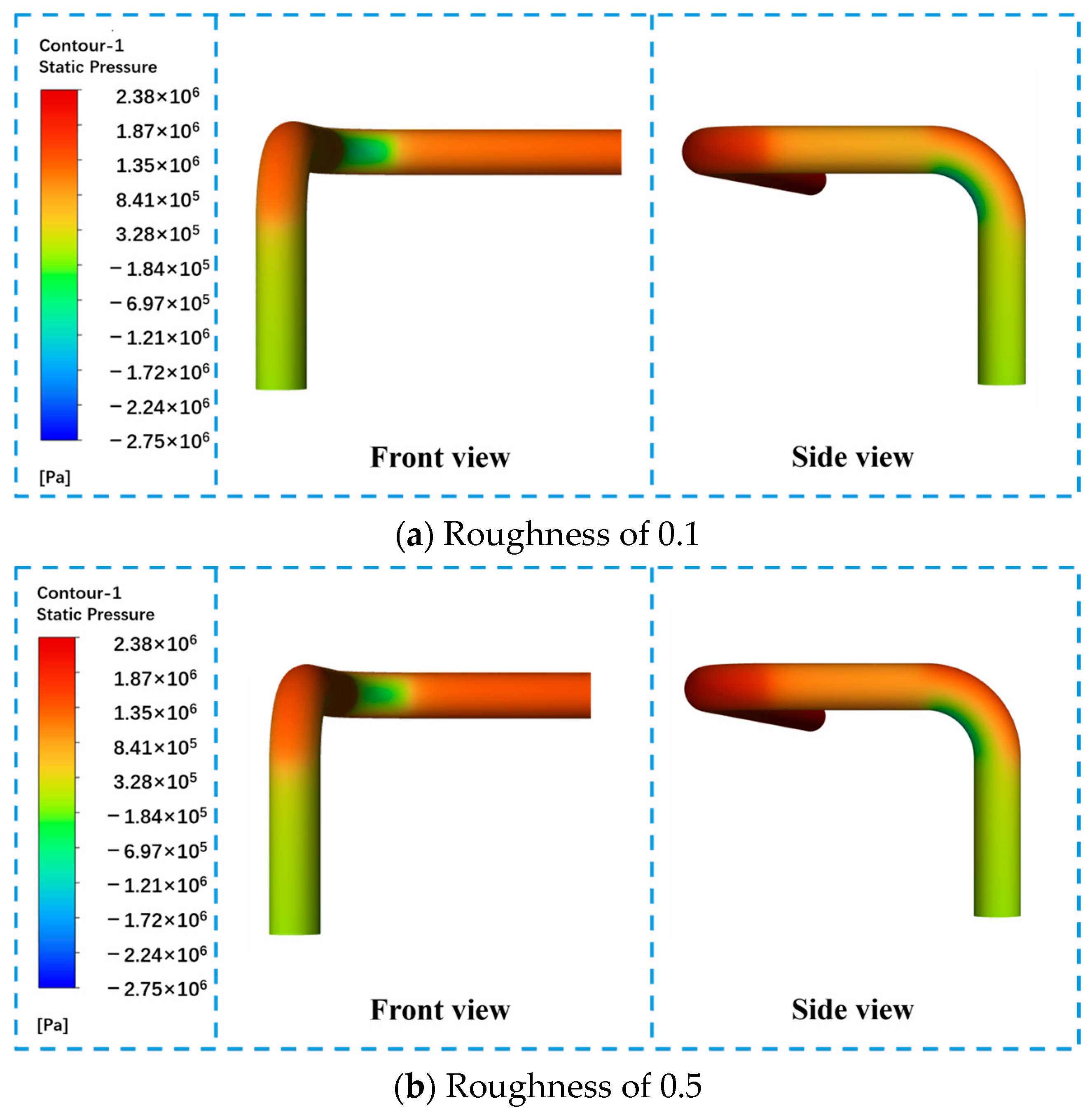
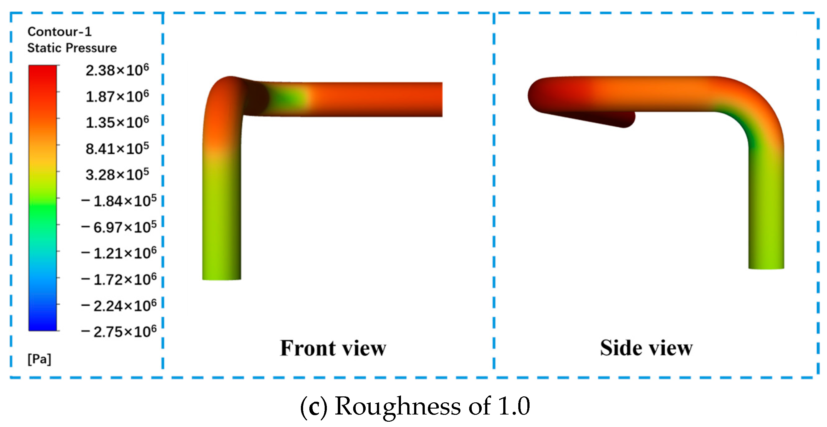
• Wall: No-slip condition applied to all pipe walls; roughness constants (0.1, 0.5, 1.0)
• defined at the bend region.
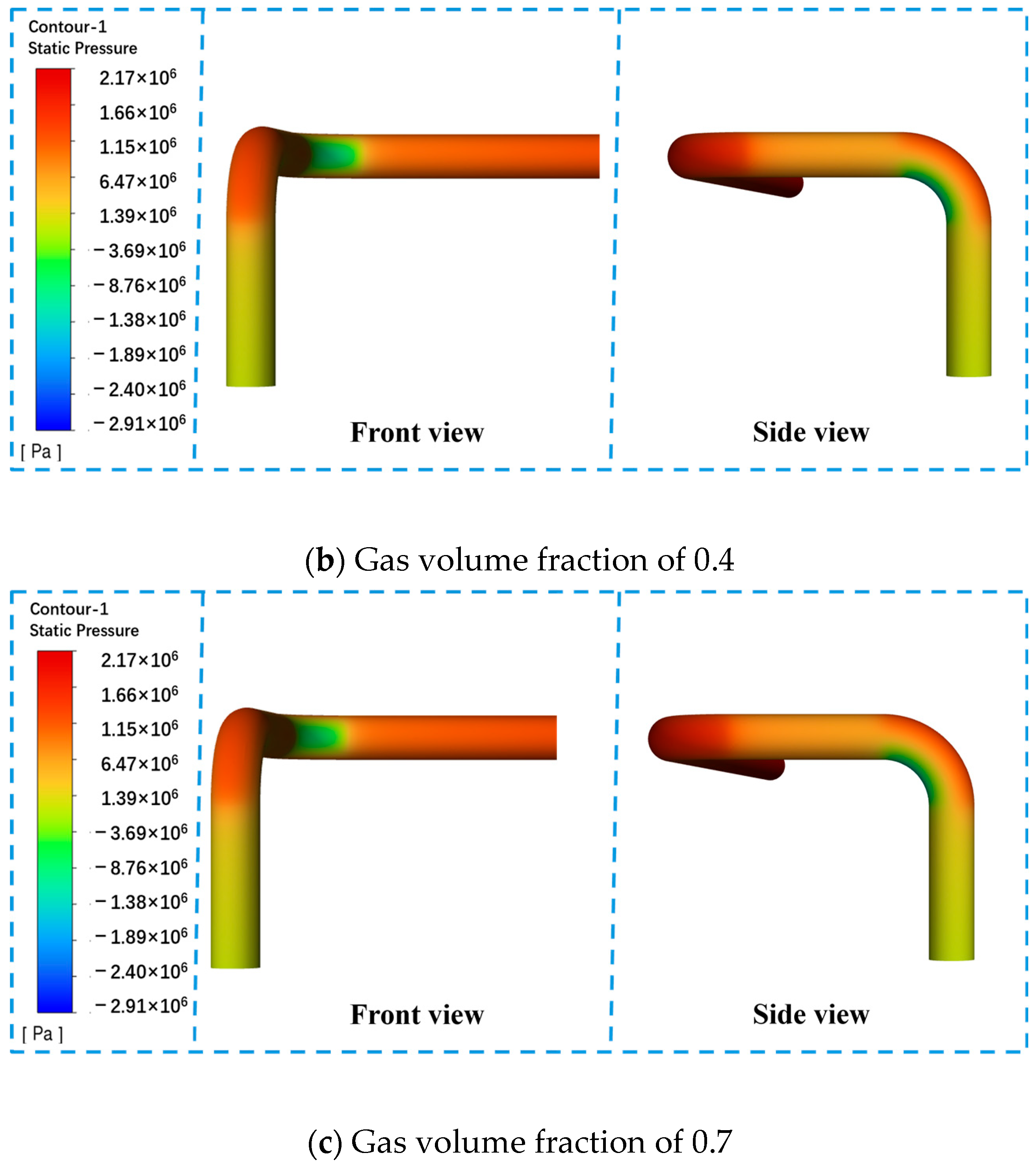
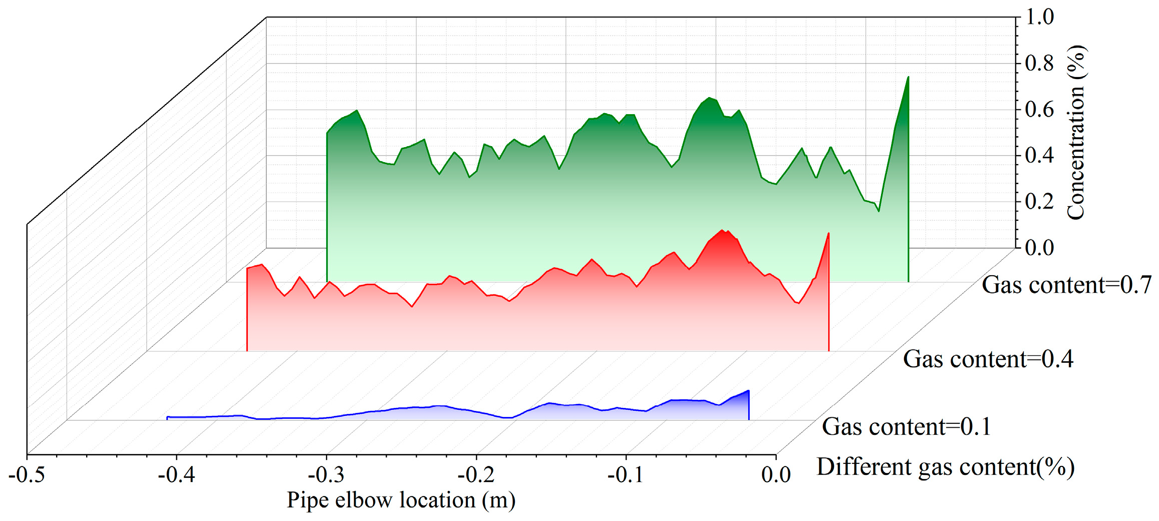
• Discrete phase: Bubble injection from the inlet with predefined mass flow rates at gas volume fractions of 10%, 40%, and 70%.
• Turbulence model: Standard RNG k–ε model with enhanced wall treatment.

Convergence was ensured by monitoring the residuals of all governing equations, which dropped below 10⁻⁵.

3. Results and Discussion

3.1. Experimental Results

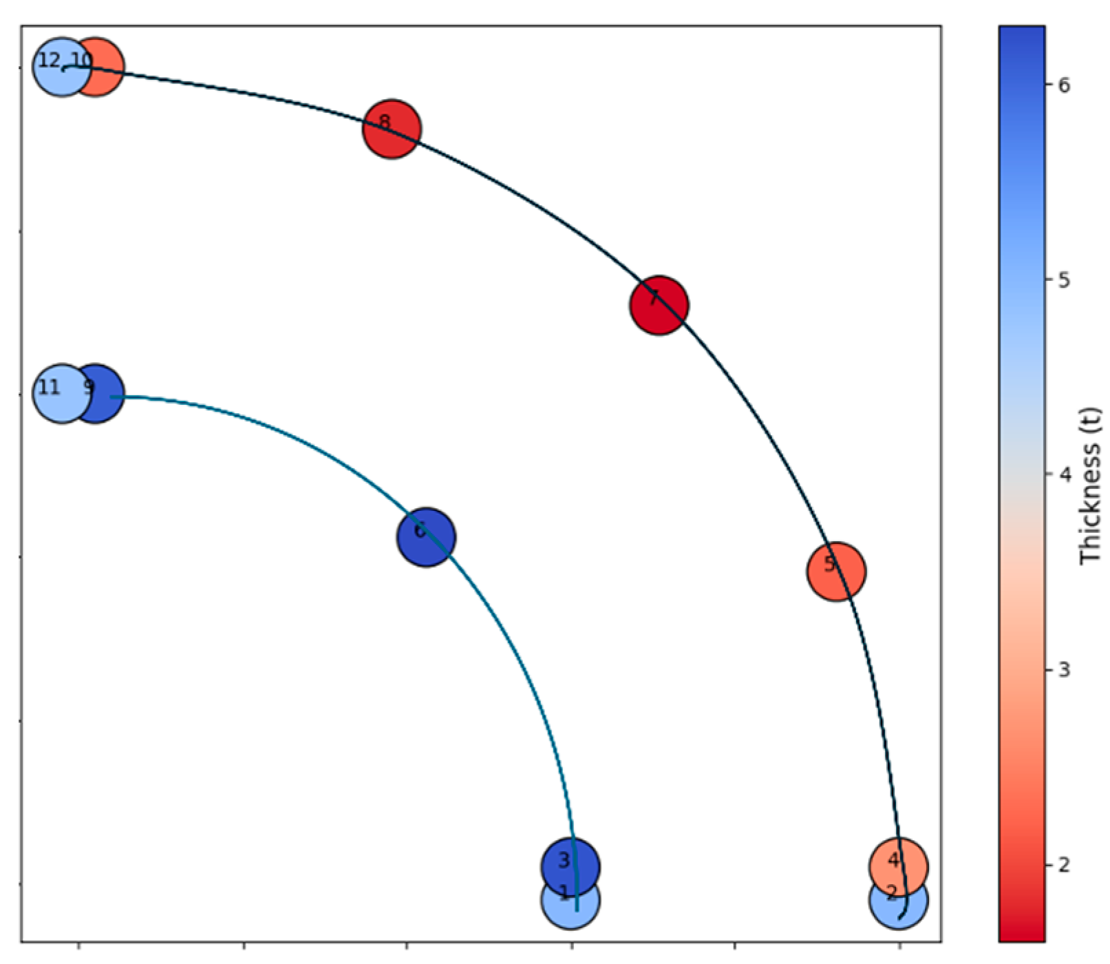
3.1.1. Wall Thickness Measurement

During field inspection of the gas–liquid two-phase flow signal tube in the power plant’s high-pressure heater, significant erosion was observed at the pipe bend. Figure 2 shows the cross-sectional view of the pipe bend with two key points marked as A and B. According to the measurement data in

Table 2. Composition and content of elbow.

Test point	1	2	3	4	5	6	7	8	9	10	11	12
Thickness (mm)	5.0	5.0	6.2	2.7	2.2	6.3	1.6	1.8	6.1	2.3	4.8	4.8

, wall thickness varies significantly between different locations: the maximum thickness is 6.3 mm (Point 6), while the minimum thickness is only 1.6 mm (Point 7), with other measurement points ranging from 2.2 mm to 6.2 mm. These data indicate that the outer side of the pipe bend (Point A) has experienced more severe erosion compared to the inner side (Point B), resulting in significant wall thinning.

Figure 3 further illustrates the distribution map of wall thickness measurements, using color coding to visually represent thickness variations, where red areas indicate thinner walls and blue areas indicate thicker walls. The 12 thickness measurement points were distributed symmetrically along the inner and outer arcs of the bend to capture differences in corrosion thinning between high-velocity and low-velocity flow zones. At the pipe bend, changes in fluid flow direction led to non-uniform velocity distribution. Due to centrifugal forces acting on the fluid along the curved path, flow velocities are generally higher on the outer side compared to the inner side. These higher velocities result in significantly increased shear stress on the outer side, leading to more severe erosion.

3.1.2. Analysis of Corrosion Cross-Sections and Surfaces

Figure 4a shows a macroscopic view of the pipe’s inner wall, which is covered with erosion pits of varying sizes and shapes. These pits are caused by localized impact forces generated when bubbles collapse on the pipe wall. Some areas exhibit erosion pits with sharp edges, similar to pitting corrosion, with visible cracks at the base of these sharp edges. Under continuous fluid impingement, these cracks gradually propagate, eventually leading to edge fracture and the formation of larger corrosion pits, accelerating metal loss and further wall thinning. Figure 4b provides a higher magnification microscopic view, focusing on details within the corrosion pits. The magnified view reveals more densely packed smaller corrosion pits, which serve as hotspots for corrosion activity and tend to accumulate corrosion products. However, fluid washing action removes these products, exposing fresh metal surfaces and perpetuating the cycle of erosion and corrosion.

As shown in Figure 4a,b, a combined analysis of the SEM images clearly reveals the erosion mechanism induced by gas–liquid two-phase flow. When high-temperature steam flows through the pipe, bubbles form on the inner wall. When these bubbles are carried away and suddenly collapse, they generate highly localized impact forces, resulting in surface depressions and cracks. Over time, these depressions and cracks gradually expand, leading to continuous metal loss. During the erosion process, corrosion products form on the metal surface, but fluid washing action removes these products, exposing new metal surfaces and maintaining the cycle of erosion and corrosion. This ongoing damage process leads to further wall thinning, correlating with the initial measurement data.

Figure 5a shows a 300× magnified image of the pipe’s inner wall surface, revealing distinctly rough surface features with significant material erosion signs around the cavities, indicating intense corrosion activity in these areas. These pits are the direct result of bubble burst impacts, where corrosion products accumulate as fluid flows past. The irregular pits and depressions clearly demonstrate erosion pits, indicating significant physical damage to the inner wall from bubble burst impacts. Figure 5b shows oxide film details at a higher magnification. The image reveals distinct irregular structures with large holes and cracks. The surface appears highly rough with significant corrosion characteristics, suggesting severe material damage during the corrosion process. These holes have irregular edges, with some areas showing signs of material delamination or erosion. These rough surface features indicate that the corrosion process involves not only physical bubble impacts but also likely chemical corrosion effects, leading to further material degradation.

A combined analysis of Figure 5a,b leads to the following conclusions: When the pipe operates in a high-temperature aqueous environment, iron atoms lose electrons to form iron ions and react with oxygen to form oxide films. However, this oxide film is loose and porous in structure, failing to effectively prevent corrosion medium penetration. Simultaneously, impact forces from bubble collapse near the wall lead to erosion pit formation, which further promotes corrosion product accumulation. The incomplete oxide film structure and the presence of erosion pits work synergistically to significantly accelerate the pipe’s corrosion process.

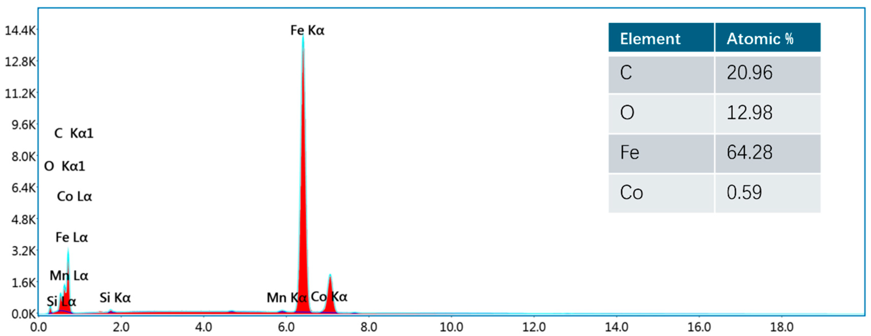
3.1.3. Energy Spectrum Analysis

Figure 6 presents two crucial EDS spectra, with Figure 5 corresponding to the uncorroded metal substrate at the pipe end and Figure 5 and Figure 6. focusing on the corrosion products. In Figure 6, a prominent Fe Kα peak highlights iron as the main component, accompanied by lower Co Lα and C Kα1 peaks, indicating the presence of cobalt and carbon in the metal substrate. In contrast, the corrosion product spectrum in Figure 5 shows a still-prominent Fe Kα peak but with significantly increased O Kα1 peak intensity, indicating oxygen-rich corrosion products, while the C Kα1 peak intensity is reduced, and the Co Kα peak remains relatively low. In the uncorroded metal substrate, carbon content reaches 68.04 At%, iron is 24.27 At%, oxygen is 7.40 At%, and cobalt is 0.29 At%. In the corrosion products, iron content increases to 64.28 At%, oxygen rises to 12.98 At%, carbon decreases to 20.96 At%, and cobalt slightly increases to 0.59 At%.

Comparing the EDS spectra in Figure 6 and Figure 7, the impact of corrosion on elemental composition is evident. The high carbon content in the uncorroded metal substrate suggests it might be high-carbon steel or a special alloy. The increased iron content and elevated oxygen levels in the corrosion products indicate the formation of iron oxides; the reduced carbon content suggests carbon combining with iron to form carbides. Although the cobalt content is low, its slight increase in the corrosion products may be due to either alloy composition changes or selective dissolution during corrosion.

The pipe bend’s outer side shows significant wall thinning, with a minimum thickness of only 1.6 mm compared to a maximum of 6.3 mm. This difference primarily results from non-uniform fluid velocity distribution at the bend. Higher flow velocities and greater centrifugal forces on the outer side lead to significantly increased shear stress, further intensifying erosion phenomena. Local impact forces from bubble collapse create erosion pits and cracks on the metal surface, with these defects gradually expanding over time.

Regarding corrosion, loose and porous oxide films were found in the corrosion pits on the pipe’s inner wall. These films failed to effectively prevent corrosion medium penetration, while bubble collapse impact forces further damaged the oxide films, exposing fresh metal surfaces and maintaining a vicious cycle of erosion and corrosion. EDS analysis revealed high carbon content in the uncorroded metal substrate, suggesting it might be high-carbon steel or a special alloy, while corrosion products showed significantly increased iron content and substantially elevated oxygen levels, indicating the formation of iron oxides such as rust or iron oxide.

SEM images further revealed the formation mechanisms of the erosion and corrosion pits. Irregular surface pits are the direct result of bubble burst impacts, while the synergistic effect of oxide film formation and bubble impacts leads to surface roughening and accelerated corrosion. Continuous bubble impacts destroy oxide films and expose fresh metal surfaces, ultimately resulting in significant wall thinning.

3.2. Experimental Results

3.2.1. Wall Thickness Measurement

Figure 8 shows the static pressure distribution of gas–liquid two-phase flow in the pipe at gas volume fractions of 0.1, 0.4, and 0.7. Each subfigure includes front and side views to clearly demonstrate pressure variations across both the pipe cross-section and length. At a 0.1 gas fraction, as shown in Figure 8a, the static pressure distribution is relatively uniform, with pressure values primarily ranging between 1.15 × 10⁶ Pa and 1.66 × 10⁶ Pa. Both front and side views show higher pressure on the pipe’s outer side and lower pressure on the inner side, indicating centrifugal force effects at the pipe bend. As the gas fraction increases to 0.4, as shown in Figure 8b, pressure distribution becomes less uniform. High-pressure regions (red) become more pronounced at the pipe bend, indicating increased flow instability due to gas phase presence. Although the overall pressure range remains between 1.15 × 10⁶ Pa and 1.66 × 10⁶ Pa, the high-pressure region area expands. When gas fraction further increases to 0.7, as shown in Figure 8c, pressure distribution becomes significantly non-uniform, with high-pressure regions more concentrated at the pipe bend. This indicates that under high gas fraction conditions, the dominant gas phase leads to significant flow instability, potentially causing larger pressure fluctuations and flow separation phenomena. As the gas fraction increases, the static pressure distribution transitions from uniform to non-uniform, especially in the pipe bend region. This phenomenon primarily results from increased flow instability due to higher gas phase proportions, affecting pressure distribution uniformity.

Pressure values were extracted along the centerline of the pipe bend’s outer side and plotted, as shown in Figure 9. As gas content increases, pressure at the pipe bend also increases. This indicates that gas content significantly influences pressure distribution at the bend. All curves show a sharp rise near the bend’s highest point, indicating a rapid pressure increase in this region. This is likely due to centrifugal forces acting on the fluid as it flows through the bend. Furthermore, higher gas content leads to faster pressure increases, particularly when approaching the bend. This may be due to higher gas content causing more bubbles or gas accumulation at the bend, resulting in increased turbulence and pressure losses.

Figure 10 shows the DPM concentration of gas–liquid two-phase flow in the pipe at gas volume fractions of 0.1, 0.4, and 0.7. Each subfigure includes front and side views to clearly demonstrate DPM concentration variations across both the pipe cross-section and length. At a 0.1 gas fraction, as shown in Figure 10a, the DPM concentration is relatively low, with most regions showing blue and green colors, indicating a low DPM concentration. This suggests fewer bubbles in the fluid, weaker turbulent effects, uniform DPM distribution, and minimal local droplet or particle deposition. As the gas fraction increases to 0.4, as shown in Figure 10b, the DPM concentration significantly increases at the bend, with colors gradually shifting to green, indicating a notable concentration elevation at the bend. This may result from decreased fluid density due to an increased gas fraction and enhanced turbulent effects from bubble breakup at the bend, leading to more droplet or particle deposition. When the gas fraction further increases to 0.7, as shown in Figure 10c, the DPM concentration rises significantly, with most regions showing red, indicating a very high DPM concentration. This phenomenon can be attributed to stronger turbulence and secondary flow effects caused by high bubble concentration, promoting more droplet or particle accumulation and deposition. With an increasing gas fraction, DPM concentration at the bend increases significantly. This indicates that bubble breakup and enhanced turbulence at the bend result in higher DPM concentration in this region, leading to more droplet or particle deposition on pipe walls, potentially accelerating the corrosion process.

The DPM concentration values were extracted along the centerline of the pipe bend’s outer side and plotted as curves showing the DPM concentration distribution at different gas fractions, as shown in Figure 11. The x-axis represents the z-coordinate values of the bend, while the y-axis shows the DPM concentration distribution along the bend’s outer wall. The graph demonstrates DPM concentration variations at different gas contents (0.1, 0.4, and 0.7). As the gas content increases, the DPM concentration shows a clear upward trend. Specifically, at 0.1 gas content, the DPM concentration remains relatively low, mainly ranging between 0.1% and 0.3% with minimal fluctuations; when the gas content increases to 0.4, the DPM concentration rises significantly, expanding to a range of 0.2% to 0.6%; as the gas content further increases to 0.7, the DPM concentration reaches its peak, fluctuating between 0.4% and 0.8%. This phenomenon indicates that higher gas content not only elevates overall DPM concentration but also intensifies its fluctuations at the bend. This may be due to enhanced turbulence and mixing effects with higher gas content, leading to increased DPM deposition at the bend. The increase in gas content significantly raises the DPM concentration at the bend and amplifies its fluctuations, primarily due to enhanced turbulence and mixing promoting greater DPM deposition.

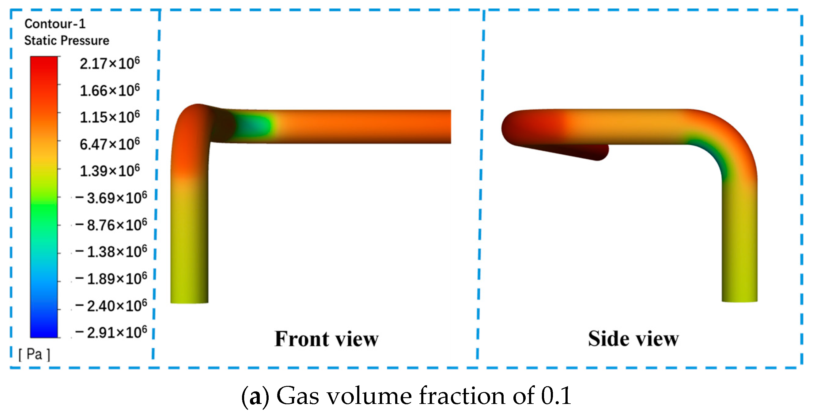
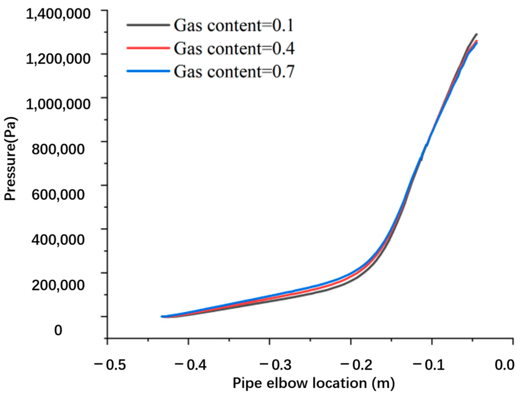
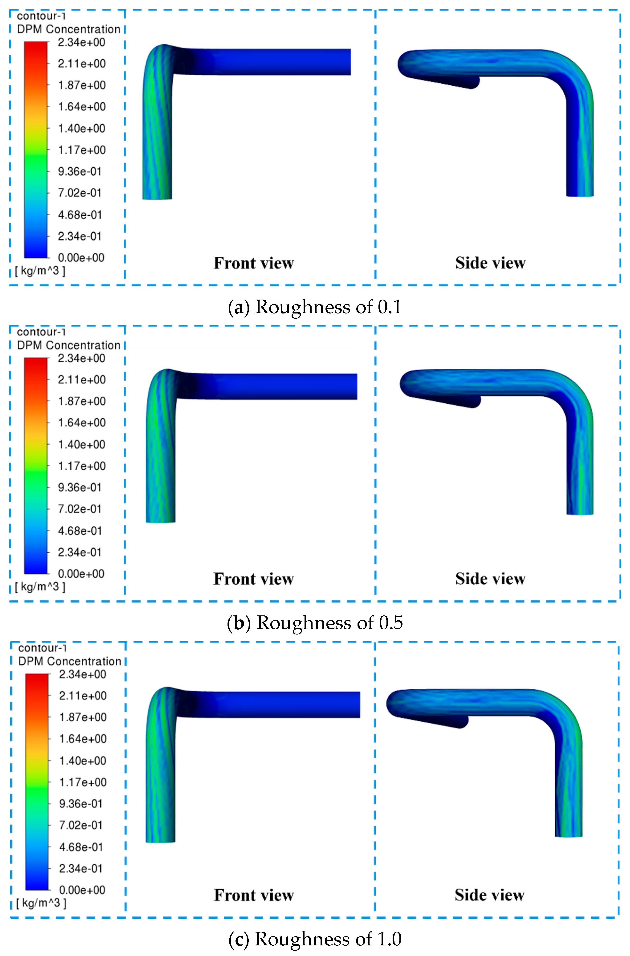
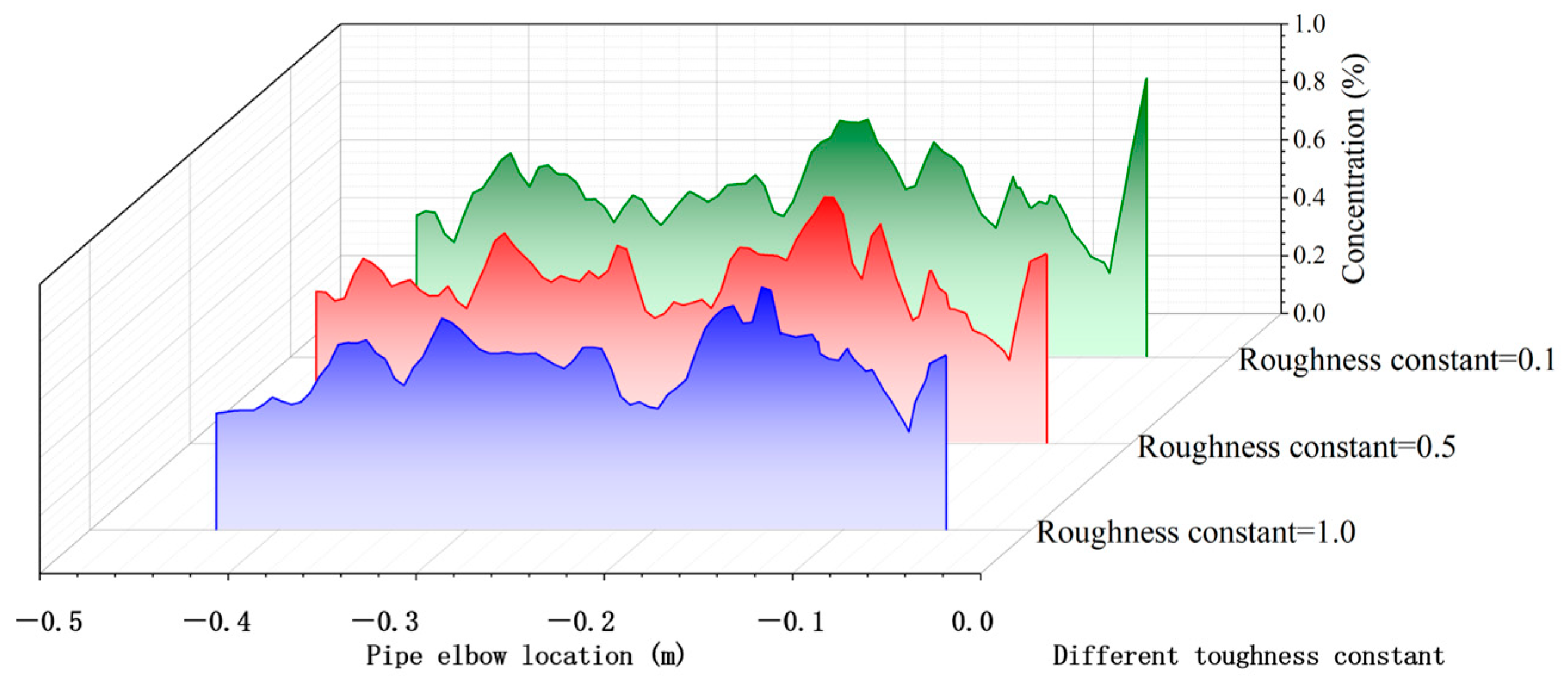
3.2.2. Effects of Pipe Bend Inner Surface Roughness on Pressure Distribution and DPM in Gas–Liquid Two-Phase Flow

Figure 12 shows the pressure distribution of gas–liquid two-phase flow within the pipe bend at different inner surface roughness values (0.1, 0.5, and 1.0). As roughness increases, pressure distribution transitions from relatively uniform to non-uniform, with significant increases in pressure peaks. Specifically, at 0.1 roughness, pressure distribution is relatively smooth, with colors transitioning from green to yellow; at 0.5 roughness, pressure gradients increase, with some areas showing red, indicating significant pressure elevation; at 1.0 roughness, pressure distribution becomes highly non-uniform, with more red regions indicating increased high-pressure areas. The color legend shows static pressure ranging from −2.75 × 10⁶ Pa to 2.38 × 10⁶ Pa. As roughness increases, maximum pressure values rise from approximately 1.87 × 10⁶ Pa to nearly 2.38 × 10⁶ Pa, while minimum pressure values remain relatively stable. This indicates that increased roughness primarily leads to higher pressure peaks while having a minimal impact on pressure minimums. Physically, increased roughness results in greater friction losses, particularly in the bend’s curved section, potentially causing flow separation and turbulence, thereby affecting overall system performance. Therefore, inner surface roughness is a key factor affecting the pressure distribution of gas–liquid two-phase flow in pipe bends. Optimizing roughness can effectively control pressure losses and flow characteristics, improving pipeline system efficiency and stability.

Figure 13 demonstrates the effect of different roughness constants on pressure distribution along the outer side of the pipe bend. The x-axis represents the bend position from 0 m to −0.5 m, with 0 m being the inlet; the y-axis shows pressure ranging from 0 to 1,600,000 Pascal. The three curves correspond to roughness constants of 0.1, 0.5, and 1.0. As the roughness constant increases, inlet pressure rises significantly. Specifically, at a roughness constant of 0.1, inlet pressure is approximately 1,200,000 Pascal; at 0.5, inlet pressure increases to about 1,400,000 Pascal; and at 1.0, inlet pressure reaches as high as 1,600,000 Pascal. This indicates that higher roughness leads to greater friction losses, resulting in higher pressure at the inlet. Furthermore, as roughness increases, pressure gradually decreases from −1.5 m to −3 m, stabilizing near −0.5 m. This may be due to changes in fluid flow characteristics at this location, such as flow separation or reattachment, leading to reduced pressure gradients. Higher roughness results in significantly increased inlet pressure and creates different pressure gradients throughout the pipe, primarily due to increased friction losses.

Figure 14 shows the DPM concentration distribution of gas–liquid two-phase flow at different pipe bend inner wall roughness values (0.1, 0.5, 1.0). Through a comparison of the front and side views, it can be clearly observed that as inner wall roughness increases, the DPM concentration rises significantly, especially in the bend region. Specifically, at 0.1 roughness, the DPM concentration is relatively low, primarily showing blue and green colors, indicating smooth flow and weak turbulent effects. When roughness increases to 0.5, DPM concentration increases significantly at the bend, with colors gradually shifting to green and yellow, showing stronger turbulent effects and more droplet or particle deposition. Further increasing roughness to 1.0, the DPM concentration rises further, with more yellow and red regions appearing in the image, indicating a very high DPM concentration and significantly enhanced turbulent effects, leading to more droplet or particle deposition at the bend. This phenomenon is mainly due to increased flow resistance from high roughness, resulting in stronger turbulence and secondary flow effects, thus promoting DPM accumulation and deposition. In conclusion, the increased inner wall roughness of the bend significantly increases DPM concentration, particularly in the bend region, which may exacerbate corrosion and wear issues, posing potential threats to pipeline system safety and stability.

Figure 15 reveals the impact of different pipe bend inner wall roughness values on the DPM concentration in gas–liquid two-phase flow. The figure presents, in three-dimensional form, the variation in DPM concentrations along the bend position under three roughness conditions: 0.1, 0.4, and 0.7. As roughness increases, the DPM concentration rises significantly, particularly in the bend region. Specifically, at 0.1 roughness, the DPM concentration remains relatively low, mainly ranging between 0.1% and 0.3% with minimal fluctuations; at 0.4 roughness, the DPM concentration increases to between 0.2% and 0.6% with larger amplitude fluctuations; at 0.7 roughness, the DPM concentration further rises to between 0.4% and 0.8% with the most significant fluctuations. This phenomenon indicates that higher inner wall roughness not only enhances turbulent effects but also leads to increased droplet or particle deposition at the bend. This is primarily due to high roughness intensifying flow turbulence, especially in flow separation regions, thereby promoting DPM accumulation and deposition. Therefore, bend inner wall roughness has a significant impact on DPM concentration distribution, particularly in the bend region.

The gas volume fraction and pipe bend inner wall surface roughness both significantly affect the pressure distribution and DPM concentration distribution in gas–liquid two-phase flow. The gas volume fraction primarily influences fluid characteristics by enhancing turbulence and centrifugal force effects, while surface roughness affects fluid behavior by altering local flow characteristics and fluid resistance.

Although this study does not explicitly define flow regimes, the observed increases in turbulence and DPM clustering with rising gas content are consistent with a transition from dispersed bubbly to slug-like patterns. These changes are influenced by increasing Reynolds and Weber numbers under higher void fractions. Ma et al. [31] similarly reported regime shifts and unsteady gas–liquid dynamics in U-bend systems, supporting the applicability of flow pattern analysis to curved-pipe erosion studies.

4. Conclusions

This study was conducted to address the insufficient understanding of how gas–liquid two-phase flow characteristics—specifically void fraction and inner wall surface roughness—contribute to corrosion-induced wall thinning in the pipe bends of high-pressure steam pipelines. Although previous works have examined flow erosion and surface degradation separately, few have explored their coupled effects using a combined experimental and CFD simulation approach. To bridge this gap, we performed wall thickness measurements and SEM/EDS analysis on in-service elbows and conducted multiphase flow simulations with varying gas content and roughness parameters to reveal the underlying flow-induced corrosion mechanisms.

The main findings of this work are as follows:

(1)

An increased void fraction significantly enhances turbulence intensity and centrifugal force effects, leading to localized pressure peaks and higher DPM (Discrete Phase Model) particle concentrations at the pipe bend, which accelerates erosion and cyclic corrosion product detachment.

(2)

Greater surface roughness disrupts flow attachment and reattachment behavior, amplifies flow instability, and shifts the location of DPM deposition upstream. This results in increased wall pressure, non-uniform distribution, and intensified local corrosion, as confirmed by SEM imaging.

(3)

The interaction of high void fraction and roughness exhibits a strong synergistic effect, where extreme pressure and DPM values are reached. This coupling amplifies erosion–corrosion mechanisms and raises the risk of rapid wall thinning, especially at critical flow regions.

This study provides new insights into the physical interaction between gas–liquid flow dynamics and corrosion behavior in curved pipelines. However, the CFD framework assumes isothermal and steady-state conditions, and further studies are needed to incorporate thermal gradients, transient flows, and actual oxide film mechanics. From an engineering perspective, these findings support the need for real-time wall thinning monitoring, predictive modeling tools, and optimized pipe design using corrosion-resistant materials and controlled flow conditions to extend service life in high-risk piping systems.

References

1. Berrichon, J.D.; Louahlia-Gualous, H.; Bandelier, P.; Bariteau, N. Experimental and theoretical investigations on condensation heat transfer at very low pressure to improve power plant efficiency. Energy Convers. Manag. 2014, 87, 539–551. [Google Scholar] [CrossRef]
2. Zhang, C.; Gallichan, R.; Leung, D.P.; Budgett, D.M.; McCormick, D. A high-precision and low-power capacitive pressure sensor interface IC with wireless power and data transfer for a pressure sensor implant. IEEE Sens. J. 2023, 23, 7105–7114. [Google Scholar] [CrossRef]
3. Rusin, A.; Tomala, M.; Łukowicz, H.; Nowak, G.; Kosman, W. On-line control of stresses in the power unit pressure elements taking account of variable heat transfer conditions. Energies 2021, 14, 4708. [Google Scholar] [CrossRef]
4. Brodov, Y.M.; Aronson, K.E.; Ryabchikov, A.Y.; Nirenshtein, M.A.; Murmanskii, I.B.; Zhelonkin, N.V. State of the art and trends in the design and operation of high- and low-pressure heaters for steam turbines at thermal and nuclear power plants in Russia and abroad: Part 2. Heater design and operation peculiarities. Therm. Eng. 2020, 67, 790–799. [Google Scholar] [CrossRef]
5. Qu, M.; Yan, X.; Wang, H.; Hei, Y.; Liu, H.; Li, Z. Energy, exergy, economic and environmental analysis of photovoltaic/thermal integrated water source heat pump water heater. Renew. Energy 2022, 194, 1084–1097. [Google Scholar] [CrossRef]
6. Zhang, L.; Li, Z.-D.; Li, K.; Li, H.-X.; Zhao, J.-F. Influence of heater thermal capacity on bubble dynamics and heat transfer in nucleate pool boiling. Appl. Therm. Eng. 2015, 88, 118–126. [Google Scholar] [CrossRef]
7. Zahedi, R.; Babaee Rad, A. Numerical and experimental simulation of gas-liquid two-phase flow in 90-degree elbow. Alexandria Eng. J. 2022, 61, 2536–2540. [Google Scholar] [CrossRef]
8. Zhang, G.; Cai, W.; Tong, B.; Sun, Y.; Hu, E. Interfacial wave of the gas-liquid two-phase flow in unsaturated reservoir pores. Colloids Surf. A Physicochem. Eng. Asp. 2023, 670, 131597. [Google Scholar] [CrossRef]
9. Dong, F.; Zhang, S.; Shi, X.; Wu, H.; Tan, C. Flow regimes identification-based multidomain features for gas-liquid two-phase flow in horizontal pipe. IEEE Trans. Instrum. Meas. 2021, 70, 1–11. [Google Scholar] [CrossRef]
10. Shao, C.; Bao, N.; Wang, S.; Zhou, J. Study on the prediction method and the flow characteristics of gas-liquid two-phase flow patterns in the suction chamber. Int. J. Numer. Methods Heat Fluid Flow 2022, 32, 2700–2718. [Google Scholar] [CrossRef]
11. Huang, X.; Zhang, L.; Zhang, R.; Chen, X.; Zhao, Y.; Yuan, S. Numerical simulation of gas-liquid two-phase flow in the micro-fracture networks in fractured reservoirs. J. Nat. Gas Sci. Eng. 2021, 94, 104101. [Google Scholar] [CrossRef]
12. Wei, N.; Xu, C.; Meng, Y.; Li, G.; Ma, X.; Liu, A. Numerical simulation of gas-liquid two-phase flow in wellbore based on drift flux model. Appl. Math. Comput. 2018, 338, 175–191. [Google Scholar] [CrossRef]
13. Guo, W.; Wang, L.; Liu, C. Prediction of gas-liquid two-phase flow rates through a vertical pipe based on thermal diffusion. Ind. Eng. Chem. Res. 2021, 60, 2686–2697. [Google Scholar] [CrossRef]
14. Xie, C.; Li, X.; Liu, Y.; Zeng, F.; Luo, C. Experimental analysis and model evaluation of gas-liquid two-phase flow through choke in a vertical tube. J. Petrol. Sci. Eng. 2022, 209, 109902. [Google Scholar] [CrossRef]
15. Sha, W.; Leng, G.; Xu, R.S.; Li, S. Numerical simulation of inlet void fraction affecting oil-gas two-phase flow characteristics in 90° elbows. J. Appl. Fluid Mech. 2024, 17, 1524–1535. [Google Scholar]
16. Chen, D.; Lin, Z. Numerical investigation of gas-liquid two-phase flow in a swirl meter. MAPAN 2021, 36, 521–532. [Google Scholar] [CrossRef]
17. Ma, Y.; Yan, G.; Scheuermann, A. Discrete bubble flow in granular porous media via multiphase computational fluid dynamic simulation. Front. Earth Sci. 2022, 10, 947625. [Google Scholar] [CrossRef]
18. Govindaraj, P.; Arun, C.S. Investigating ovality and wall-thinning behaviors in free-form bending of thin pipe bends with varying guider length and roller die diameter. J. Braz. Soc. Mech. Sci. Eng. 2023, 45, 605. [Google Scholar] [CrossRef]
19. Li, W.; Liu, W.; Liu, H.; Ma, Z.; Hu, G.; Song, J.; Wang, T.; Zhang, Y.; Zhang, H. Effect of different powers on microstructure evolution and corrosion behavior of 5SiC-Ni60 coatings by directed energy deposition. Opt. Laser Technol. 2025, 180, 111456. [Google Scholar] [CrossRef]
20. Dyck, O.; Almutlaq, J.; Lingerfelt, D.; Swett, J.L.; Oxley, M.P.; Huang, B.; Lupini, A.R.; Englund, D.; Jesse, S. Direct imaging of electron density with a scanning transmission electron microscope. Nat. Commun. 2023, 14, 7550. [Google Scholar] [CrossRef]
21. Li, X.; Tian, R.; He, L.; Lv, Y.; Zhou, S.; Li, Y. A novel numerical approach for assessing the gas-liquid flow characteristics in pipelines utilizing a two-fluid model. Appl. Math. Model. 2024, 131, 233–252. [Google Scholar] [CrossRef]
22. Marrocos, P.H.; Fernandes, I.S.; Pituco, M.M.; Lopes, J.C.B.; Dias, M.M.; Santos, R.J.; Vilar, V.J.P. CFD and lower order mechanistic models for gas-liquid flow in NETmix: Pressure drop and gas hold-up. Chem. Eng. Sci. 2024, 284, 119478. [Google Scholar] [CrossRef]
23. Hao, L.; Zhai, X.W.; Wang, K. Study on the diffusion characteristics of small hole leakage of high-sulfur natural gas in gathering and transmission pipelines. Int. Commun. Heat Mass Transf. 2025, 164, 108942. [Google Scholar] [CrossRef]
24. Zhang, P.; Ma, L.; Sun, J.; Chen, R.; Pei, G.; Chen, X.; Fan, J. Numerical investigation of air flow field evolution and leakage patterns in large-scale goaf areas. Phys. Fluids 2025, 37, 027151. [Google Scholar] [CrossRef]
25. Niño, L.; Gelves, R.; Ali, H.; Solsvik, J.; Jakobsen, H. Applicability of a modified breakage and coalescence model based on the complete turbulence spectrum concept for CFD simulation of gas-liquid mass transfer in a stirred tank reactor. Chem. Eng. Sci. 2020, 211, 115272. [Google Scholar] [CrossRef]
26. Shirzadi, M.; Mirzaei, P.A.; Naghashzadegan, M. Improvement of k-epsilon turbulence model for CFD simulation of atmospheric boundary layer around a high-rise building using stochastic optimization and Monte Carlo sampling technique. J. Wind Eng. Ind. Aerodyn. 2017, 171, 366–379. [Google Scholar] [CrossRef]
27. Anand, S.; Chambe, J.E.; Bouvet, C.; Rivallant, S. Stacking sequence optimization of composite tubes submitted to crushing using the discrete ply model (DPM). Mech. Adv. Mater. Struct. 2024, 31, 820–833. [Google Scholar] [CrossRef]
28. Zhang, J.; Wei, S.; Yue, P.; Kulik, A.S.; Li, G. Surface pressure calculation method of multi-field coupling mechanism under the action of flow field. Symmetry 2023, 15, 1064. [Google Scholar] [CrossRef]
29. Chen, H.; Sun, Z.; Li, Y.; Su, H. Simulation of flow and heat transfer in high-temperature and high-pressure reservoir based on multi-physical field coupling model at pore scale. Can. J. Chem. Eng. 2025, 103, 914–926. [Google Scholar] [CrossRef]
30. Hu, R.; Fang, F.; Salinas, P.; Pain, C.C.; Sto. Domingo, N.D.; Mark, O. Numerical simulation of floods from multiple sources using an adaptive anisotropic unstructured mesh method. Adv. Water Resour. 2019, 123, 173–188. [Google Scholar] [CrossRef]
31. Ma, X.; Gu, Z.; Ni, D.; Li, C.; Zhang, W.; Zhang, F.; Tian, M. Experimental study on gas-liquid two-phase flow upstream and downstream of U-bends. Processes 2024, 12, 277. [Google Scholar] [CrossRef]
Figure 1. Model mesh partition diagram.
Processes 13 02096 g001
Figure 2. Cross-section of erosion thinning in signal pipe bend.
Processes 13 02096 g002
Figure 3. Schematic diagram of wall thickness measurement points for the pipe bend. Points 1–6 are located on the outer arc, and points 7–12 are located on the inner arc of the bend.
Processes 13 02096 g003
Figure 4. SEM images of eroded cross-section.
Processes 13 02096 g004
Figure 5. SEM of the corroded surface of the pipe’s inner wall.
Processes 13 02096 g005
Figure 6. EDS energy spectrum analysis of pipe section.
Processes 13 02096 g006
Figure 7. EDS spectrum analysis of corroded surface.
Processes 13 02096 g007
Figure 8. Pressure distribution of gas–liquid two-phase flow at different gas contents.
Processes 13 02096 g008aProcesses 13 02096 g008b
Figure 9. Pressure values of bends with different gas content.
Processes 13 02096 g009
Figure 10. DPM of gas–liquid two-phase flow with different gas contents.
Processes 13 02096 g010
Figure 11. Elbow DPM values at different pressures.
Processes 13 02096 g011
Figure 12. Pressure distribution of gas–liquid two-phase flow at different roughness constants.
Processes 13 02096 g012aProcesses 13 02096 g012b
Figure 13. Pressure values on the outer side of elbows with different roughness constants.
Processes 13 02096 g013
Figure 14. DPM of gas–liquid two-phase flow in bends with different inner wall roughness constants.
Processes 13 02096 g014
Figure 15. DPM of gas–liquid two-phase flow in bends with different inner wall roughness.
Processes 13 02096 g015