
A Hybrid Data-Cleansing Framework Integrating Physical Constraints and Anomaly Detection for Ship Maintenance-Cost Prediction via Enhanced Ant Colony–Random Forest Optimization


Abstract
1. Introduction
1.1. Research Background
1.2. Research Motivation
1.2.1. Engineering-Oriented Reengineering of Conventional Anomaly Detection Frameworks
- Redundancy-Type Anomalies. These arise from spatiotemporal synchronization errors in multi-sensor systems or the simultaneous operation of parallel support systems. They typically manifest as duplicate work order records and redundant attribute fields. For instance, Data Rows 1 and 2 contain fully identical records for a -class vessel repair.
- Contradiction-Type Anomalies. These manifest as logical conflicts between hull physical parameters and fluid dynamics characteristics. Examples include combinations of vessel length, beam, and displacement that violate ship statics constraints, or main engine power and maximum speed deviating from theoretical calculation ranges. A typical case is Data Row 8, which records a -class vessel with a displacement of 8000 tons and a main engine power of 75,000 kW, yet lists a speed of 55 knots—far exceeding the established reasonable range (where vessels of comparable tonnage typically achieve speeds ≤30 knots). This necessitates verification for potential data-entry errors or sensor malfunction.
- Discrete-Type Anomalies. These exhibit abrupt, high-amplitude characteristics, typically manifesting as non-continuous, abnormal distributions in key parameters. For example, Data Row 3 records a -class vessel with a displacement of 32,000 tons and a length of 85 m—a combination far exceeding the reasonable dimensions for comparable vessels (where the actual displacement should be approximately 3200 tons).
- Missing-Type Anomalies. These present multimodal characteristics, including the absence of critical parameters and discontinuous maintenance records, as exemplified by Data Rows 4 and 6.
1.2.2. Multidimensional Challenges in Conventional Data Cleansing
- Statistical Methodology Limitations: Conventional statistical approaches—including boxplot analysis and the three-sigma criterion—demonstrate diminishing efficacy when confronted with nonlinear interdependencies among multisource parameters, failing to detect latent anomalies due to their reliance on identical distribution assumptions. Yao et al. critically identified the inadequacy of conventional boxplot methods in complex marine engineering scenarios, pioneering a LOF-IDW hybrid methodology for integrated anomaly detection and rectification. This approach demonstrated a 27.6% average reduction in the data coefficient of variation post-cleansing through field validations on offshore platform monitoring systems [9]. In parallel, Zhu innovatively employed K-dimensional tree spatial indexing to characterize distributed photovoltaic plant topologies, synergizing enhanced three-sigma criteria to elevate high-reliability data ratios from 43.61% to 85.71% in grid-connected power quality analysis [10].
- Insufficient Sensitivity of Clustering Algorithms: Conventional clustering algorithms such as DBSCAN and K-means exhibit limited detection accuracy for anomalies in unevenly distributed density spaces, leading to erroneous cleansing of critical fault precursors. Song et al. enhanced DBSCAN density clustering through STL to decompose time-series trends and periodicity, achieving precision and recall rates of 0.91 and 0.81, respectively, for DO and pH anomaly detection in marine environmental monitoring [11]. In parallel, Han developed a hybrid data-cleansing strategy that integrates Tukey’s method with threshold constraints coupled with K-means clustering to optimize wind-speed-to-power characteristic curve fitting, resulting in an improved R2 value of 0.99 for cleansed datasets [12].
- Machine-Learning Models’ Disregard for Physical Constraints: While algorithms such as Isolation Forest (iForest) and Local Outlier Factor (LOF) demonstrate robust general-purpose anomaly detection capabilities, their lack of integration with domain-specific physical constraints remains a critical limitation. Liu et al. extracted four coarse-grained type-level features and three fine-grained method-level features, reframing software defect identification as an anomaly detection task using iForest. This approach achieved an average runtime of 21 min across five open-source software systems while reducing false positive rates by 75% [13]. Shen et al. further enhanced robustness through a soft-voting ensemble combining PCA-Kmeans, the Gaussian Mixture Model (GMM), and iForest, supplemented by a Gradient Boosting Decision-tree (GBDT)-based imputation model, attaining 99.1% precision and 95.9% recall [14]. However, these methods exhibit a fundamental flaw: their repair logic remains decoupled from equipment physics, risking physically implausible restoration outcomes under real-world operating conditions.
1.3. Research Innovations
- Construction of a Physics-Driven Constraint Knowledge Base: This study pioneers the systematic encoding of ship hydrodynamics, structural mechanics, and maintenance operational protocols into a quantifiable constraint system. By establishing a multidimensional engineering–physical correlation network, we enable effective identification of contradiction-type anomalies while ensuring the cleansed data aligns with authentic vessel operating conditions.
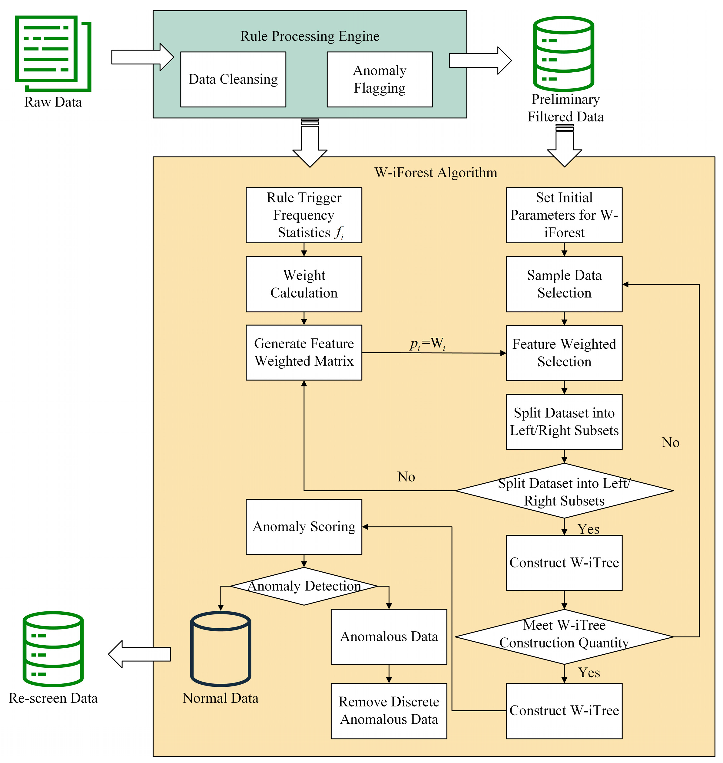
- Design of a Feature-Weighted Isolation Forest Algorithm (W-iForest): We propose a dynamic weight allocation mechanism integrating rule-triggering frequency and expert knowledge to enhance the feature selection strategy of the iForest algorithm. By prioritizing the partitioning of highly sensitive parameters, this innovation significantly improves the detection efficiency for discrete-type anomalies.
- Development of a Genetic Algorithm-Ant Colony Optimization Collaborative Random Forest (GA-ACO-RF) Missing Data Imputation Model: This innovation synergizes Genetic Algorithms (GA) and Ant Colony Optimization (ACO) to dynamically adapt Random Forest (RF) hyperparameters. By leveraging GA to initialize ACO pheromone concentrations, we integrate GA’s global search capabilities with ACO’s local optimization strengths, effectively escaping local optima traps in high-dimensional missing data imputation.
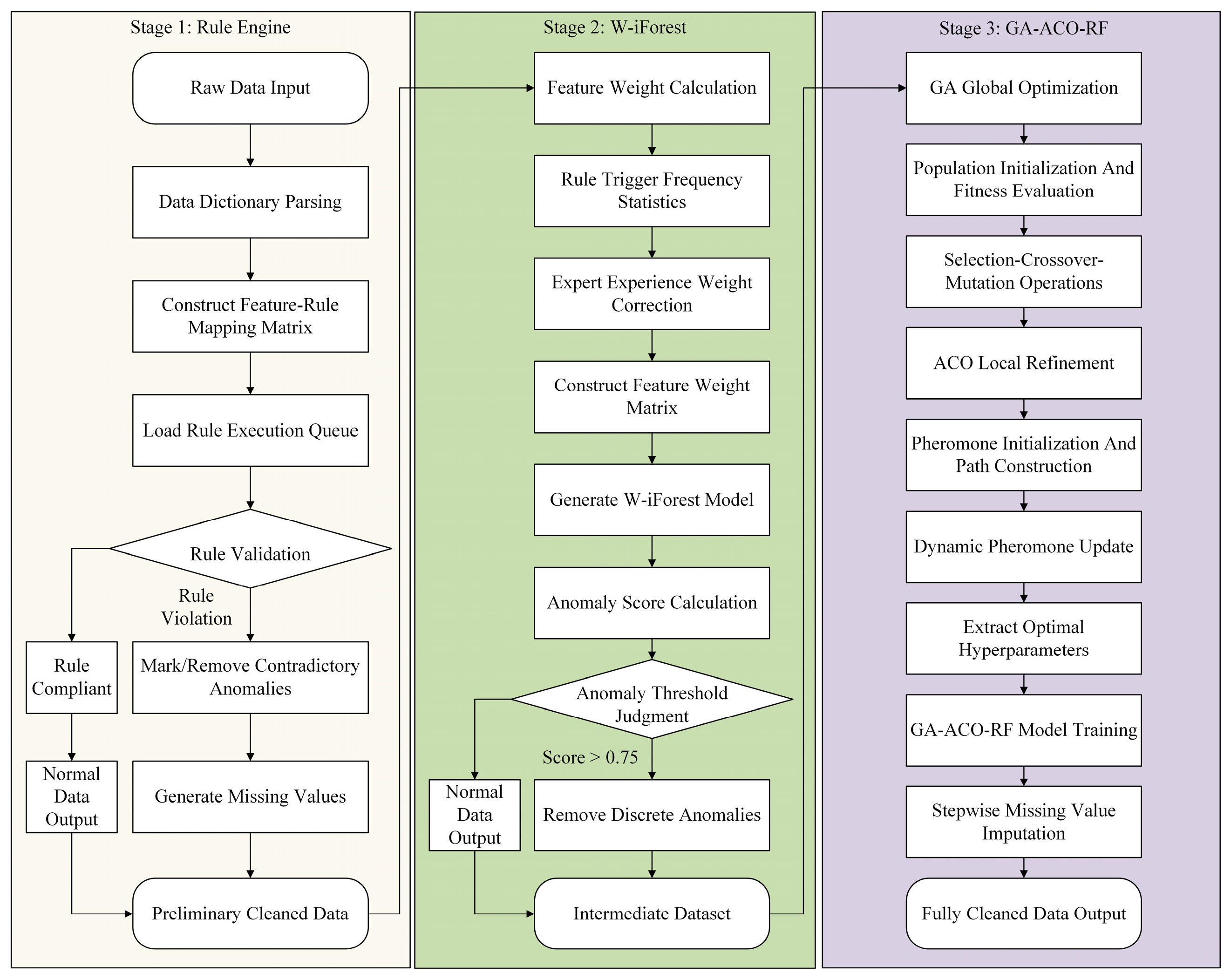
- Establishment of a Multimodal Collaborative Cleansing Framework: We pioneer a three-stage closed-loop architecture: (1) Rule-Based Pre-Filtering, (2) W-iForest Anomaly Elimination, and (3) GA-ACO-RF Intelligent Imputation. This integrated framework achieves coordinated governance of contradiction-, discrete-, and missing-type anomalies, enabling generation of high-quality datasets with 88.2% physical compliance rates—a 25% improvement over conventional methods.
1.4. Research Structure
- Section 2 comprehensively reviews advancements in data-cleansing methodologies, focusing on the evolutionary trajectories and existing bottlenecks of anomaly detection and imputation techniques.
- Section 3 proposes an innovative methodology framework, including (1) the construction of a marine engineering physical constraint knowledge base, (2) the design of the W-iForest anomaly detection algorithm, and (3) the development of the GA-ACO-RF missing value imputation model.
- Section 4 conducts empirical validation using multi-type vessel maintenance datasets, verifying model superiority through comparative experiments and ablation studies.
- Section 5 summarizes research findings and practical engineering applications, critically analyzes current limitations, and outlines future research directions.
2. Related Work
2.1. Evolution and Comparative Analysis of Outlier Detection Techniques
- Statistical Analysis-Based Detection Methods: Statistical detection methods establish threshold boundaries through the mathematical characterization of data distributions to quantitatively identify outliers. Classical algorithms include the three-sigma rule under Gaussian distribution assumptions, the IQR-based box plot method, and the extreme value theory-driven Grubbs’ test. These approaches demonstrate advantages in computational efficiency and low algorithmic complexity, making them particularly suitable for rapid cleansing of univariate datasets. Huang Guodong applied the three-sigma rule to cleanse univariate time-series data from water supply network pressure monitoring. By eliminating data points deviating beyond the mean range, an anomaly detection accuracy rate of 89% was achieved [20]. However, these limitations have become increasingly evident in complex industrial scenarios. First, algorithmic efficacy heavily relies on assumptions about data distribution patterns, leading to systematic misjudgments in non-Gaussian distributions. A representative case involves wind turbine operational data where Tip-speed Ratio (TSR) parameters typically exhibit multimodal mixture distribution characteristics. Under such conditions, the normality-assumption-based criterion erroneously flags 22–35% of operational mode transition points [21]. Second, traditional statistical methods fail to capture implicit correlations among multivariates. When processing strongly coupled multidimensional data, independent single-dimensional cleansing disrupts physical constraint relationships among parameters, resulting in the misclassification of normal operational fluctuations as anomalies. Empirical studies demonstrate that when cleansing 12-dimensional datasets from coal-fired power plant SCR denitrification systems, the false detection rate of box plot methods reaches 41.7%, significantly higher than association analysis-based machine-learning approaches [22].
- Density-Based Detection Methods: Density-based detection methods overcome the limitations of traditional statistical approaches reliant on global distribution assumptions by identifying anomalies through local neighborhood density variations. Current mainstream techniques primarily encompass two classical algorithms: DBSCAN and LOF. DBSCAN employs spatial density partitioning mechanisms, distinguishing core points, border points, and noise points, achieving anomaly localization through outlier detection in cluster-excluded discrete points. Cui Xiufang developed a density-reachable model with dynamic neighborhood parameters for maritime AIS data-cleansing requirements, successfully attaining 92.7% detection accuracy in berthing point identification and navigation trajectory anomaly detection [23]. LOF addresses anomaly detection challenges in non-uniform data distributions by calculating local density deviations between target points and their k-nearest neighbors. In water-quality monitoring, Chen innovatively integrated STL time-series decomposition with LOF algorithms, establishing a three-stage sensor noise filtration mechanism that achieved precise elimination of temporal anomalies [11]. The core advantage of these methods lies in their self-adaptive capability to identify sparse anomalies within locally dense regions without presupposing data distributions. Meng Lingwen successfully detected equipment anomalies under asynchronous operational conditions through density clustering in multi-parameter monitoring of power grid equipment [24]. Nevertheless, practical applications face significant challenges. DBSCAN exhibits parameter coupling effects between the neighborhood radius and the minimum points. Liu Jianghao’s cybersecurity intrusion detection study using the KDD CUP99 dataset demonstrated that optimal parameter combinations require determination through grid search optimization to address algorithmic sensitivity [25]. LOF confronts neighborhood-scale sensitivity, where k-value selection critically influences density calculation reliability. This necessitates cross-validation to identify optimal neighborhood scales, balancing the trade-off between detection sensitivity and false alarm rates.
- Machine-Learning-Based Anomaly Detection: This methodology achieves automated identification by establishing mapping relationships between data features and anomaly labels, broadly categorized into supervised and unsupervised learning paradigms. Within supervised learning frameworks, algorithms such as Support Vector Machines (SVM) and RF require comprehensively labeled training datasets to construct classification models. A representative application involves Han Honggui’s development of an enhanced SVM kernel function to construct a dissolved oxygen anomaly classifier for wastewater treatment processes, achieving a detection performance with an F1-score of 0.91 on industrial datasets [26]. Unsupervised methods, with iForest as a representative approach, enable rapid detection by constructing binary tree structures through random feature selection, leveraging anomalies’ susceptibility to isolation in feature spaces. Yang Haineng implemented this algorithm for power-curve cleansing in wind turbine SCADA systems, demonstrating a 40% improvement in computational efficiency compared to traditional IQR methods [27]. Current research demonstrates that these algorithms exhibit significant advantages in multi-source heterogeneous data-processing scenarios, such as multi-parameter monitoring of power grid equipment, with their detection accuracy and automation levels surpassing traditional threshold-based methods [28]. However, supervised learning confronts annotation cost challenges in domains like medical diagnostics, where data-labeling quality directly impacts model generalization capabilities [29]. While unsupervised methods reduce data dependency, they suffer from difficulties in tracing erroneous anomaly determinations. For instance, false elimination phenomena during SCADA system cleansing in wind power applications reveal how the black-box nature of decision-making logic impedes fault diagnosis implementation in industrial settings [30].
- Deep-Learning-Based Detection Methods: Deep-learning models demonstrate superior feature representation capabilities in complex scenarios through their deep neural architectures. Temporal models represented by the Long Short-Term Memory (LSTM) and Transformer architectures effectively capture temporal dependency features via gated mechanisms and attention networks. Xu Xiaogang’s developed Dual-Channel DLSTM achieved dynamic residual threshold optimization in steam turbine operational data prediction, constraining reconstruction errors within 0.5% [31]. For spatially correlated data, GNNs establish feature propagation paths through neighborhood information aggregation mechanisms. Li Li’s GCN-LSTM hybrid architecture, leveraging topological correlations among wind farm turbine clusters, accomplished wind speed anomaly cleansing with a 23% reduction in MAE [19]. Autoencoders (AEs) construct essential feature spaces via encoder–decoder frameworks. Zhao Dan employed Stacked Denoising Autoencoders (SDAEs) to process mine ventilation datasets, maintaining a 96% reconstruction accuracy under noise interference [32]. Such algorithms transcend the limitations of conventional approaches, demonstrating enhanced capabilities in processing high-dimensional unstructured data like images and texts while exhibiting distinct advantages in feature abstraction. Current research confronts two primary challenges: First, the heavy reliance on computational resources for model training, as evidenced by Liu Jianghao’s experiments revealing that DLSTM model training exceeds 12 h per session, with GPU memory consumption reaching 32GB [25]. Second, heightened sensitivity to data quality, with Peng Bo’s findings indicating reconstruction distortion in autoencoders when the signal-to-noise ratio falls below 15 dB, accompanied by an error propagation coefficient of 1.8 [33].
2.2. Evolution and Comparison of Missing Value Imputation Techniques
- Traditional Imputation Methods: Traditional imputation methods are grounded in mathematical–statistical principles and primarily include univariate imputation and time-series interpolation. Univariate imputation fills missing values using central tendency metrics such as mean/median/mode. For instance, Liu Xin applied industry-standard temperature range mean imputation to blast-furnace molten iron temperature data with a missing rate <5%, effectively maintaining the stability of metallurgical process models [34]. Time-series interpolation encompasses linear interpolation, cubic spline interpolation, and ARIMA predictive imputation. Zhu Youchan employed cubic spline interpolation to restore 12 h data gaps caused by sensor failures in distribution network voltage sequences, achieving successful reconstruction [35]. These methods demonstrate advantages in terms of low computational complexity and applicability to small-scale structured data. However, they exhibit dual limitations: (1) The univariate processing paradigm neglects inter-feature correlations. When strong coupling relationships exist between photovoltaic power output and variables like irradiance and temperature, simple mean imputation introduces systematic bias [36]. (2) Sensitivity to non-random missing scenarios. Chen et al. demonstrated that traditional interpolation applied to continuous missing segments caused by sensor failures in water-quality monitoring generates spurious stationarity artifacts, leading to a 38% misjudgment rate in subsequent water-quality alert models [37].
- Statistical Model-Based Imputation Methods: Statistical modeling approaches enable multivariate inference of missing values by establishing data distribution assumptions. Multiple Imputation (MI) generates multiple complete datasets via Markov Chain Monte Carlo (MCMC) algorithms, reducing statistical inference uncertainty through imputation result integration. Jäger’s comparative experiments under Missing at Random (MAR) mechanisms revealed that MI achieves a 23.6% reduction in RMSE compared to five imputation methods (including K-means and RF), demonstrating superior accuracy [38]. Matrix Completion Methods (MCM) leverage low-rank matrix assumptions to recover missing values through nuclear norm minimization. Zhang innovatively combined sliding window mechanisms with MCM for real-time dynamic imputation of chemical process monitoring sensor data, achieving an 18.3% reduction in imputation error [39]. These methods’ principal advantage resides in effectively preserving datasets’ statistical properties, particularly suited for structured data types with defined characteristic patterns. In power load forecasting, Liu Qingchan’s application of MI methodology to handle temporal data gaps successfully maintained the load curve’s periodic characteristics [40]. However, two critical limitations must be acknowledged: (1) Sensitivity to missing data mechanisms. Maharana’s empirical analysis revealed that under Missing Not at Random (MNAR) conditions, MI suffers imputation accuracy degradation of up to 47% [41]. (2) Computational inefficiency in high-dimensional spaces. Gu Juping’s experimental observations indicated that matrix completion operations on 10,000-dimensional power grid datasets exceeded 24 h, severely constraining real-time processing capabilities [28].
- Machine-Learning-Based Imputation Methods: Machine-learning models with nonlinear mapping mechanisms provide innovative solutions for missing data problems. Ensemble learning approaches, notably RF and XGBoost, enhance prediction accuracy through collaborative multi-decision-tree modeling. Peng Bo’s IRF algorithm achieved breakthroughs in multivariate joint imputation for photovoltaic energy systems, elevating the coefficient of determination (R2) to 0.93, outperforming conventional methods [33]. Generative models like Generative Adversarial Networks (GANs) and Variational Autoencoders (VAEs) produce realistic imputations by learning latent data distributions. Kiran Maharana’s VAE-based medical image restoration system attained a structural similarity index of 0.88 in reconstructing missing knee MRI regions, meeting clinical usability thresholds [41]. For temporal data characteristics, deep architectures such as LSTM and Transformer exhibit dynamic forecasting superiority. Wang Haining’s attention-guided LSTM achieved industry-leading performance in photovoltaic power output gap prediction with a MAPE of 2.1%, reducing errors by 47% compared to traditional time-series models [36]. These algorithms demonstrate exceptional performance in complex scenarios like smart grid systems. Liu Qingchan successfully implemented them for joint imputation of multi-source heterogeneous grid data, validating the algorithms’ capability to capture nonlinear correlations [40]. However, their double-edged nature requires prudent consideration. Mohammed’s research highlights that over-engineered architectures necessitate countermeasures like dropout mechanisms and regularization strategies to mitigate overfitting [42]. Côté warns that the black-box nature of generative models demands interpretability validation mechanisms when applied to regulated fields like finance and healthcare [29].
2.3. Limitations of Existing Research and Improvement Strategies
3. Methodology
3.1. Multi-Dimensional Constraint-Based Rule Engine System
3.1.1. Physics-Constrained Rule Base
3.1.2. Operational-Constrained Rule Base
3.1.3. Rule Engine System
- Step 1: Data Dictionary Parsing. Decoding the field attributes and business semantics of raw data through a data dictionary, establishing a feature-rule mapping relationship matrix.
- Step 2: Rule Execution Queue Construction. Generating rule execution queues based on the mapping matrix, supporting real-time loading of rule definition files.
- Step 3: Sliding Window Processing. Implementing sequential scanning of data records using a window sliding mechanism, performing syntax validation, range detection, and logical verification operations.
- Step 4: Anomaly Handling. Eliminating identified conflicting anomalies and tagging them as missing values, ultimately generating a quality report containing cleansing metadata.
3.2. Feature-Weighted Isolation Forest Algorithm
3.2.1. Isolation Forest Algorithm Principles
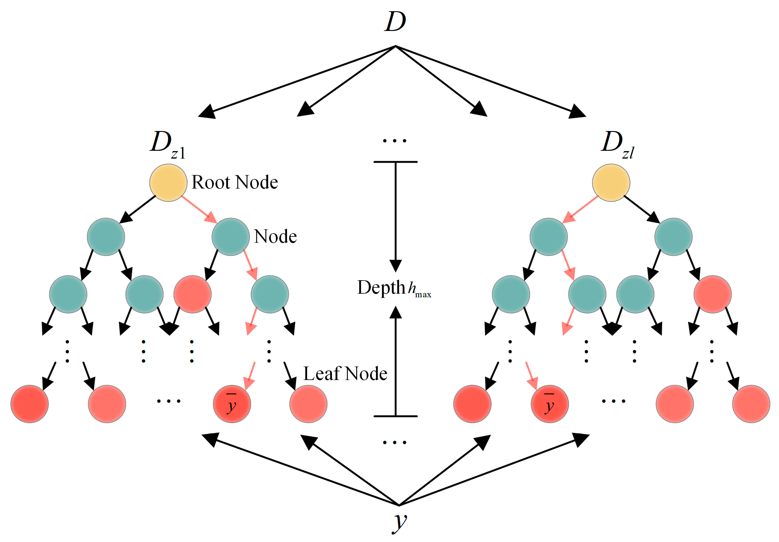
- Definition: iTrees. An iTree, as the fundamental unit of the iForest, is a specialized decision tree based on a binary tree structure [48]. Node T within the tree is classified into two types: leaf nodes without child nodes and internal nodes containing two child nodes (, ). During initialization, the root node encompasses the entire training dataset. At each split, a feature dimension is randomly selected, and a split threshold is randomly chosen within the value range of dimension . The data in the current node are partitioned into the left subtree if , with the remaining data assigned to the right subtree . The partitioning process is recursively executed until it meets any of the following termination conditions: (1) a leaf node contains only one data instance, (2) the tree depth reaches a predefined maximum threshold, or (3) all samples in the current node share identical values across the selected feature dimensions. Normal samples, clustered in high-density regions, require multiple partitioning iterations for isolation, whereas anomalies—owing to their sparse distribution—are typically isolated rapidly.
- Definition: Path Length. The path length of a data sample is defined as the number of edges traversed from the root node to the leaf node during the tree traversal. This metric reflects the isolation difficulty of samples in the feature space, where anomalies exhibit significantly shorter path lengths than normal samples due to their sparse distribution.
- Definition: Anomaly Score. Based on binary search tree theory, the normalized path length for an -sample dataset can be calculated as shown in Equation (2).
- When approaches , approaches 0.5. The sample resides at the decision boundary between anomalies and normal data, making classification indeterminate.
- When approaches 0, approaches 1. The sample is identified as a significant anomaly.
- When approaches , approaches 0. The sample is classified as normal.
3.2.2. Enhanced Isolation Forest Algorithm
- Step 1: Establish a feature-to-rule trigger mapping matrix based on the rule execution workflow in Section 3.1.3, dynamically updating each feature’s anomaly trigger frequency .
- Step 2: Compute the feature weight matrix using Equation (4) and integrate it into the iForest model.
- Step 3: During the construction of each iTree, the probability of selecting a feature for node splitting is set as , ensuring priority partitioning of critical parameters.
- Step 4: Calculate anomaly scores via weighted path lengths (Equation (3)), then eliminate outliers by combining data validity and missingness criteria. Samples with scores >0.75 and missing data are replaced with zeros.
3.3. Genetic Algorithm–Ant Colony Optimization Collaborative Random Forest Algorithm
3.3.1. Random Forest Regression Principles
- Step 1: Bootstrap Sampling. The Bootstrap resampling method is employed to perform sampling with replacement from the training set . Each iteration extracts a subsample matrix with the same dimensions as the original dataset () to train the -th regression tree (), where denotes the number of features, and represents the number of data samples per feature.
- Step 2: Randomized Feature Space Partitioning. (1) Feature Randomization. At each non-leaf node of every decision tree, features () are randomly selected without replacement from the -dimensional feature space. (2) Optimal Split Point Selection. For each candidate feature, candidate split points are randomly selected to construct an -dimensional split point matrix . (3) Splitting Criterion Calculation. The Classification and Regression Tree (CART) algorithm’s squared error minimization criterion is applied to compute loss function values for all candidate split points.
- Step 3: Decision-Tree Growth Control. The splitting process from Step 2 is repeated for each child node until any termination condition is met: (1) the node depth reaches a predefined maximum, (2) the node sample count falls below a set minimum, or (3) the squared error reduction within the node becomes smaller than a critical threshold.
- Step 4: Forest Ensemble Construction. Steps 1–3 are iteratively executed to generate structurally diverse regression trees. Each tree’s prediction is the mean value of training samples in its leaf node region. The final Random Forest output is the average of all tree predictions as Equation (8).
3.3.2. Enhanced Random Forest Algorithm
- Step 1: Parameter Initialization. Configure algorithm initialization parameters based on optimization problem characteristics. GA parameters: selection strategy, crossover probability , mutation probability , and maximum iterations . ACO parameters: initial pheromone concentration , ant colony size , pheromone evaporation coefficient , and objective function error threshold .
- Step 2: Fitness Function Design. Utilize pheromone concentration as the fitness evaluation metric for the genetic algorithm. The fitness function must satisfy the following: function outputs are non-negative and uniquely mapped, controllable time complexity, and strict alignment with optimization goals. The probability of the -th ant selecting element from set during path selection is determined by Equation (12). After all ants complete their path searches, individual fitness values are computed based on pheromone concentrations.
- Step 3: Solution Space Construction and Dynamic Pheromone Update. Initialize ant search paths and set a dynamic selection rate . Randomly select individuals to construct a candidate solution set. Perform local search optimization using the current optimal solution as the benchmark, conducting neighborhood searches via Equation (13):
- Step 4: Genetic Operation Optimization. Perform roulette wheel selection based on fitness values, employing a single-point crossover operator to exchange genetic material at randomly selected crossover points within the sorted population. Introduce Gaussian mutation operators to generate new individuals via Equations (16) and (17):
- Step 5: Iterative Convergence Check. Terminate and output the current global optimal solution if the maximum iteration count is reached; otherwise, return to Step 4 for further optimization.
- Step 6: Global Pheromone Update. Initialize the ACO algorithm’s pheromone distribution with the optimal concentrations derived from GA, enhancing population diversity.
- Step 7: State Transition Probability Calculation. Determine the transition probability for the -th ant moving from node to at time using Equation (18):
- Step 8: Iterative Pheromone Update. Dynamically adjust pheromone concentrations per Step 3 rules, establishing a positive feedback optimization loop.
- Step 9: Global Optimum Verification. Compare current and historical optimal solutions. Terminate if convergence criteria are satisfied; otherwise, repeat Steps 7–8.
- Step 10: Random Forest Model Training. Train the RF model using optimized hyperparameters (n_estimators, max_depth, min_samples_split, min_samples_leaf) with five-fold cross-validation for performance evaluation.
3.4. Hybrid Data-Cleansing Framework
4. Case Analysis and Discussion
4.1. Data Sources
4.2. Case Study
4.2.1. Outlier Detection
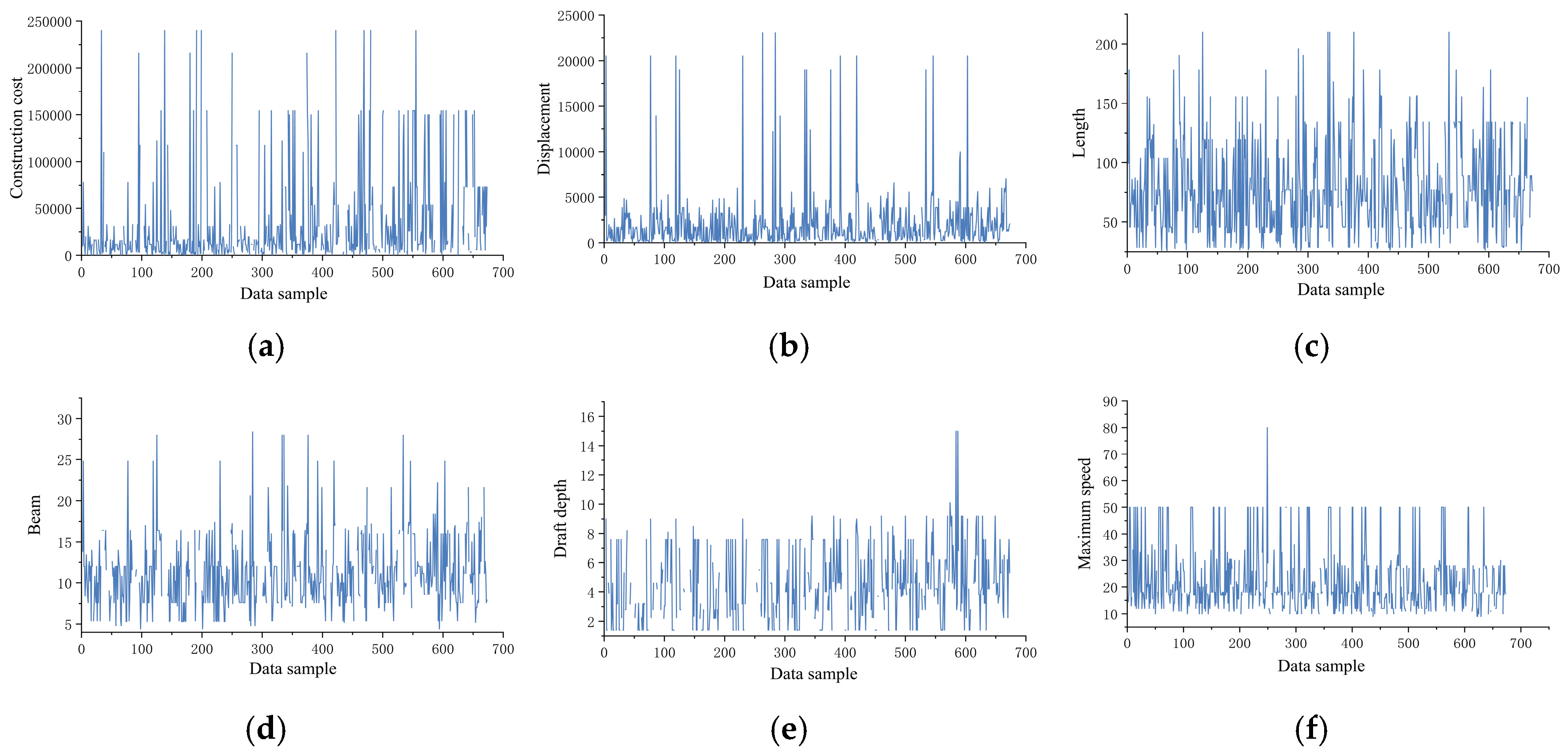
- Step 1: Rule Engine Preliminary Screening. Systematic cleansing and anomaly identification were performed on vessel maintenance data, with visualization results presented in Figure 9. Given the multidimensional characteristics of the dataset, the cleansing process focused on five core validation rules: displacement verification, speed–power relationship analysis, length–beam ratio constraints, person-hour efficiency evaluation, and cost correlation checks. Rule engine monitoring revealed that speed–power anomalies (38.64% triggering frequency) and displacement exceedances (34.86% triggering frequency) constituted the predominant anomaly types. Data provenance analysis identified two primary root causes of anomalies: (1) Missing principal dimension parameters. The absence of critical vessel principal dimensions prevented accurate calculation of displacement threshold ranges. Given that displacement serves as a key input variable for speed–power equations, such data anomalies triggered cascading effects across related parameters. (2) Propulsion system misreporting. Certain shipyards incorrectly reported “main engine power” as single-engine rated power rather than total vessel propulsion power, reflecting a systemic misunderstanding of powerplant specifications. Following multidimensional anomaly determination protocols, data instances violating ≥4 rules were classified as severe anomalies. Statistical analysis revealed 40 severe contradictory anomalies, accounting for 5.94% of the total dataset.
- Step 2: W-iForest Weighted Optimization. The W-iForest algorithm was applied for secondary data cleansing, utilizing a recursive spatial partitioning strategy to identify and eliminate discrete anomalies, thereby constructing a dataset containing missing values (null fields were temporarily populated with zeros). Based on cleansing results from the rule engine and domain expertise, six physical parameters—main engine power, maximum speed, length, beam, displacement, and draft depth—were identified as critical features and assigned an expert experience weight coefficient of 1, while all other parameters received a weight coefficient of 0.
- Step 3: Feature Weight Calculation. The feature weight for each variable is calculated via Equation (4), incorporating three key elements: (a) the frequency of anomaly triggers within the rule repository for each feature, (b) rule-type weighting factors (confidence level: 0.6 for physical constraint rules, 0.4 for operational rules), and (c) expert knowledge correction coefficients. To elucidate the weight allocation mechanism, consider a streamlined dataset example with three features: main engine power, vessel length, and maintenance cycle. Within the rule repository, their anomaly trigger frequencies are 12, 8, and 2 occurrences, respectively. Both engine power and vessel length are physical constraint rules (weight of 0.6), while the maintenance cycle is an operational rule (weight of 0.4), with expert correction coefficients uniformly set at 1.0. Unnormalized weights are calculated as follows: engine power is , vessel length is , and maintenance cycle is . Normalization yields final weights: engine power is , vessel length is , and maintenance cycle is . This demonstrates how physical parameters attain significantly higher weights due to both frequent rule triggering and higher rule-type weighting. Actual feature weight distributions for ship-maintenance data are presented in Table 6.
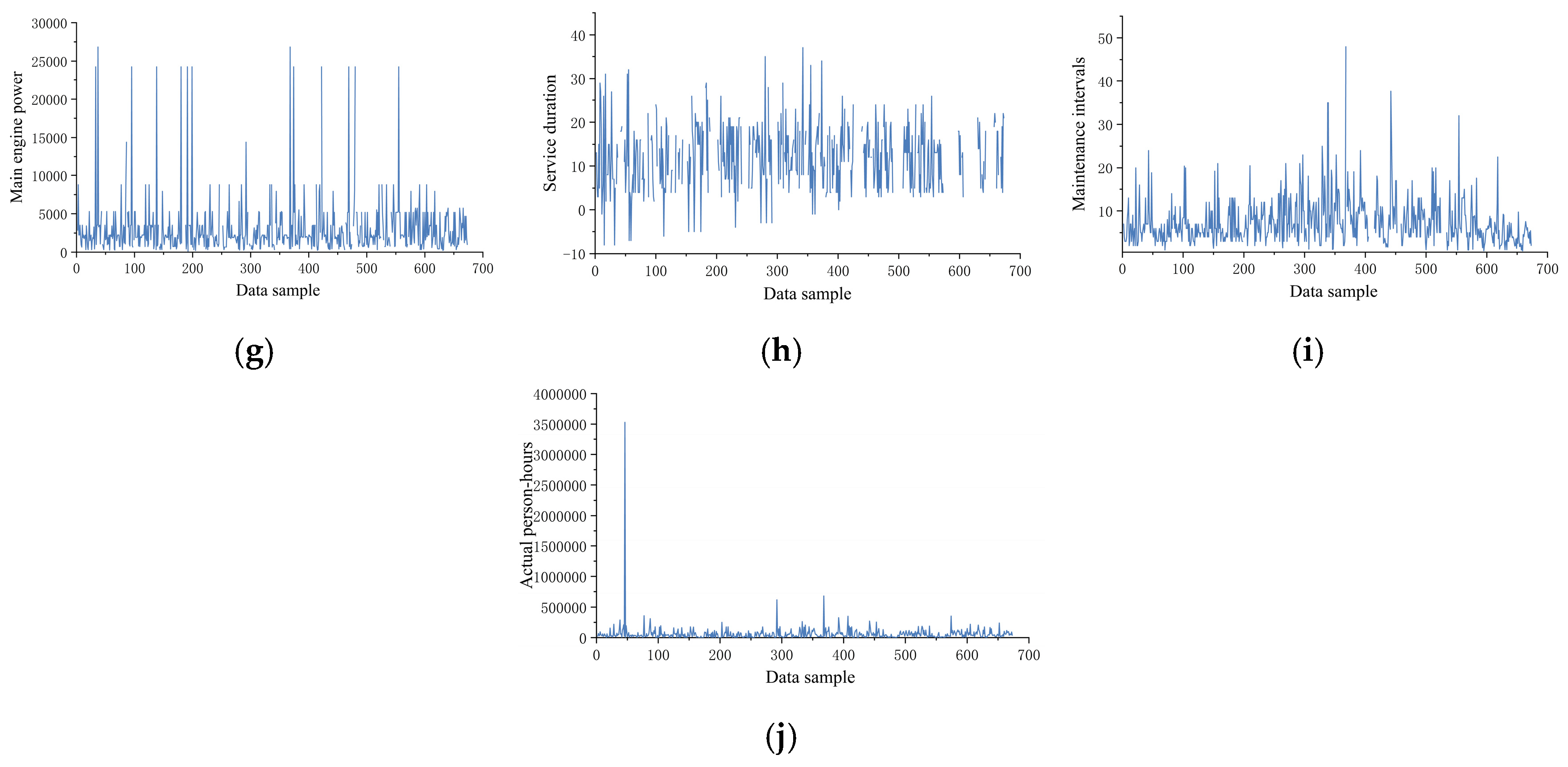
- Step 4: Anomaly Detection and Validation. By setting the anomaly threshold >0.75, the W-iForest algorithm detected 67 additional anomalous samples (9.95% of the total dataset), spanning 10 variables, including construction cost and actual person-hours. Post-cleansing via the rule base and W-iForest algorithm, the data distributions of all variables are visualized in Figure 10.
4.2.2. Missing Value Imputation
- Step 1: Missing Pattern Analysis. Using Python 3.12 64-bit, the missing values in the two-stage cleansed dataset were visualized. Figure 11 illustrates the quantity and distribution of missing values across variables. The parameters with the highest missing counts are draft depth (310 entries), in-service duration during maintenance (209 entries), construction cost (127 entries), maximum speed (120 entries), and main engine power (58 entries).
- Step 2: GA-ACO-RF Collaborative Optimization. This study proposes a GA-ACO-RF imputation method that achieves high-precision missing data compensation through a multi-algorithm collaborative mechanism. GA achieves targeted propagation of high-quality genes through a high crossover probability () while maintaining population diversity with a mutation probability (); ACO employs a dynamic pheromone evaporation rate ( = 0.5) to autonomously adjust search directions, coupled with a heuristic weight factor ( = 2) to strengthen critical feature identification; RF suppresses overfitting via synergistic constraints (max_depth = 11 and min_samples_leaf = 1), while the parameter configuration n_estimators = 191 enhances computational efficiency without compromising model precision.
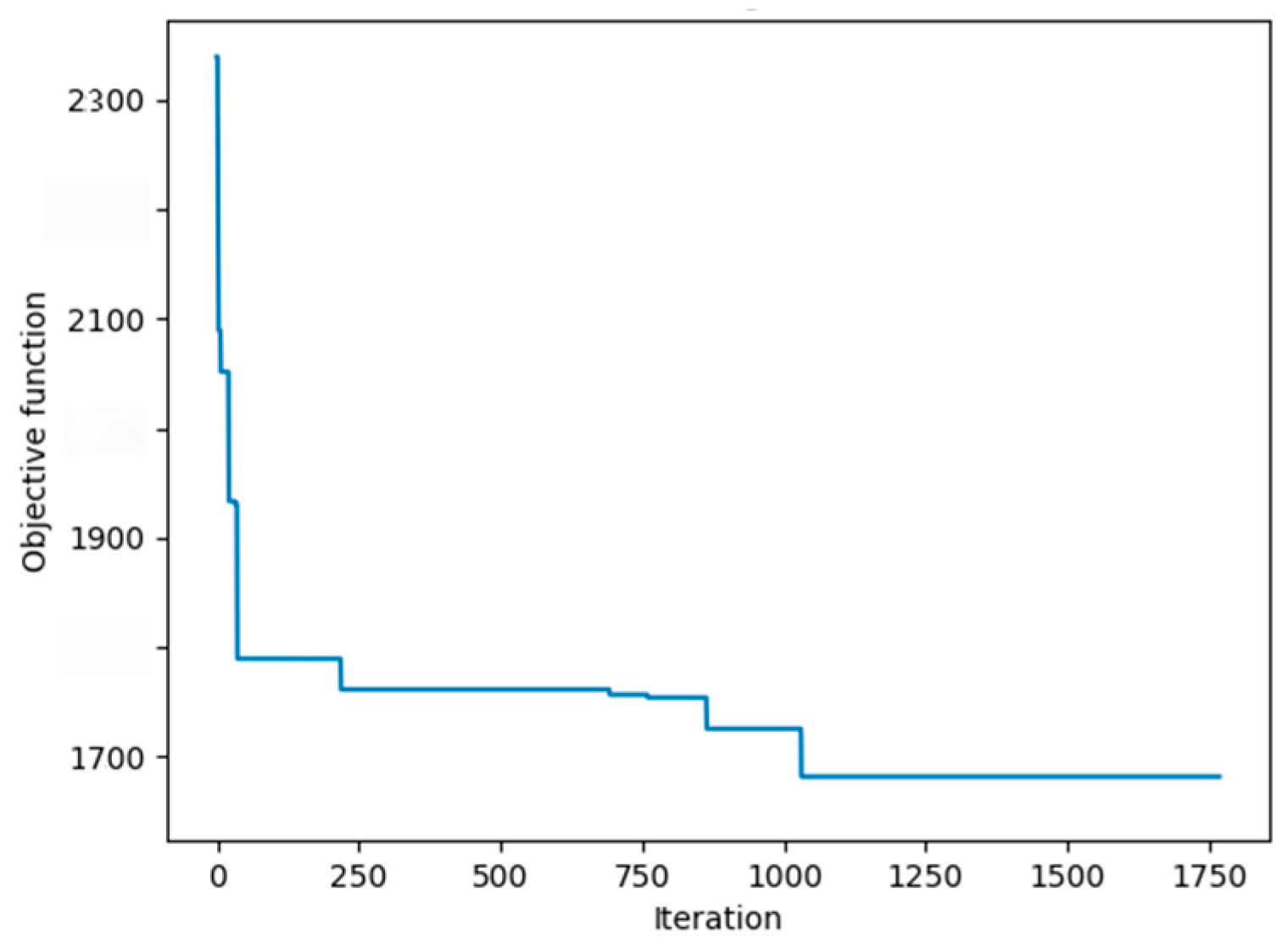
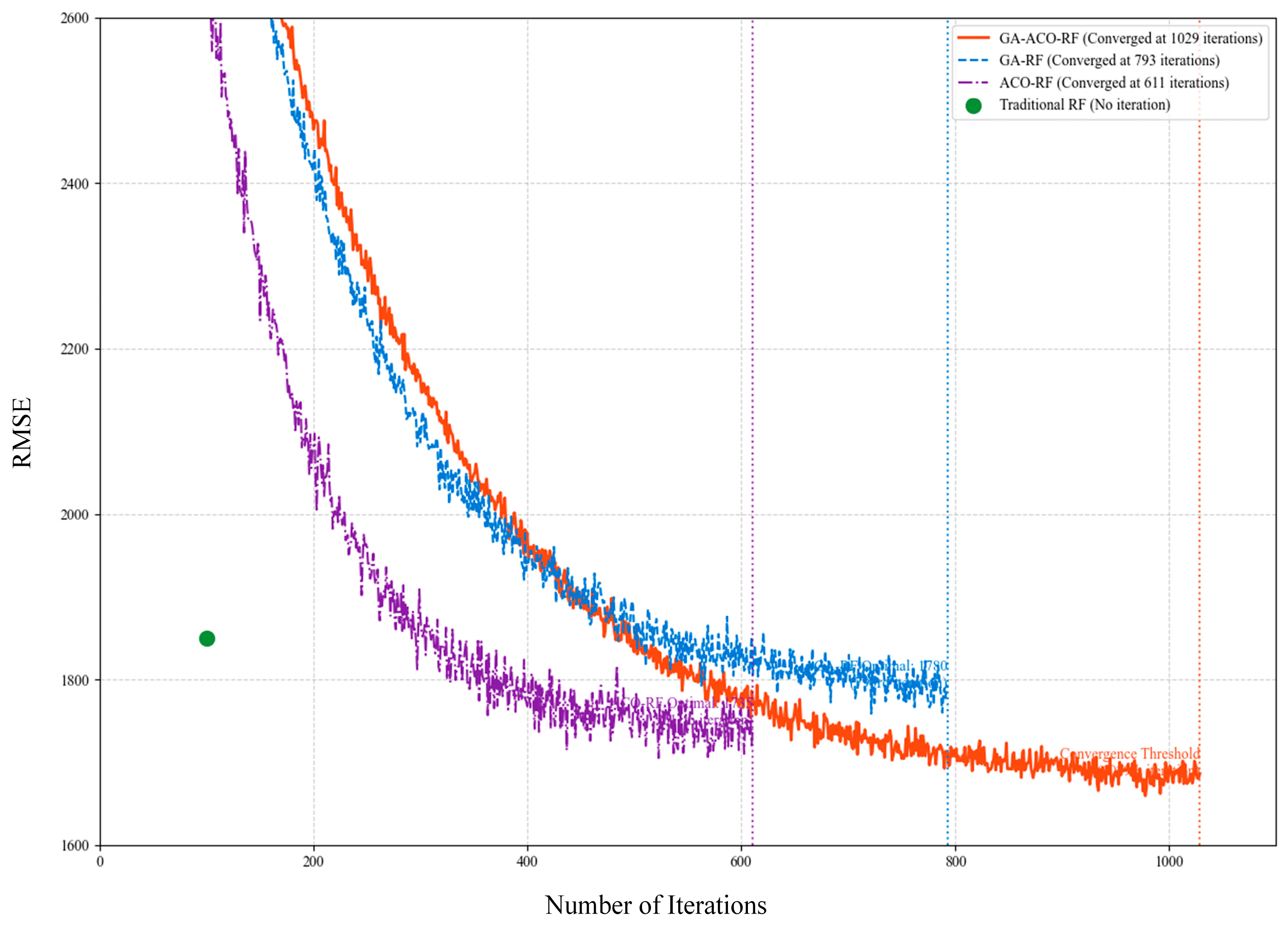
- Step 3: Hyperparameter Convergence Validation. The optimal parameter combination presented in Table 7 reveals the collaborative mechanism of multiple algorithms. The convergence curve shown in Figure 12 demonstrates that the algorithm reached the convergence threshold at 1029 iterations. At this point, the obtained hyperparameter combination achieves optimal imputation accuracy for the model.
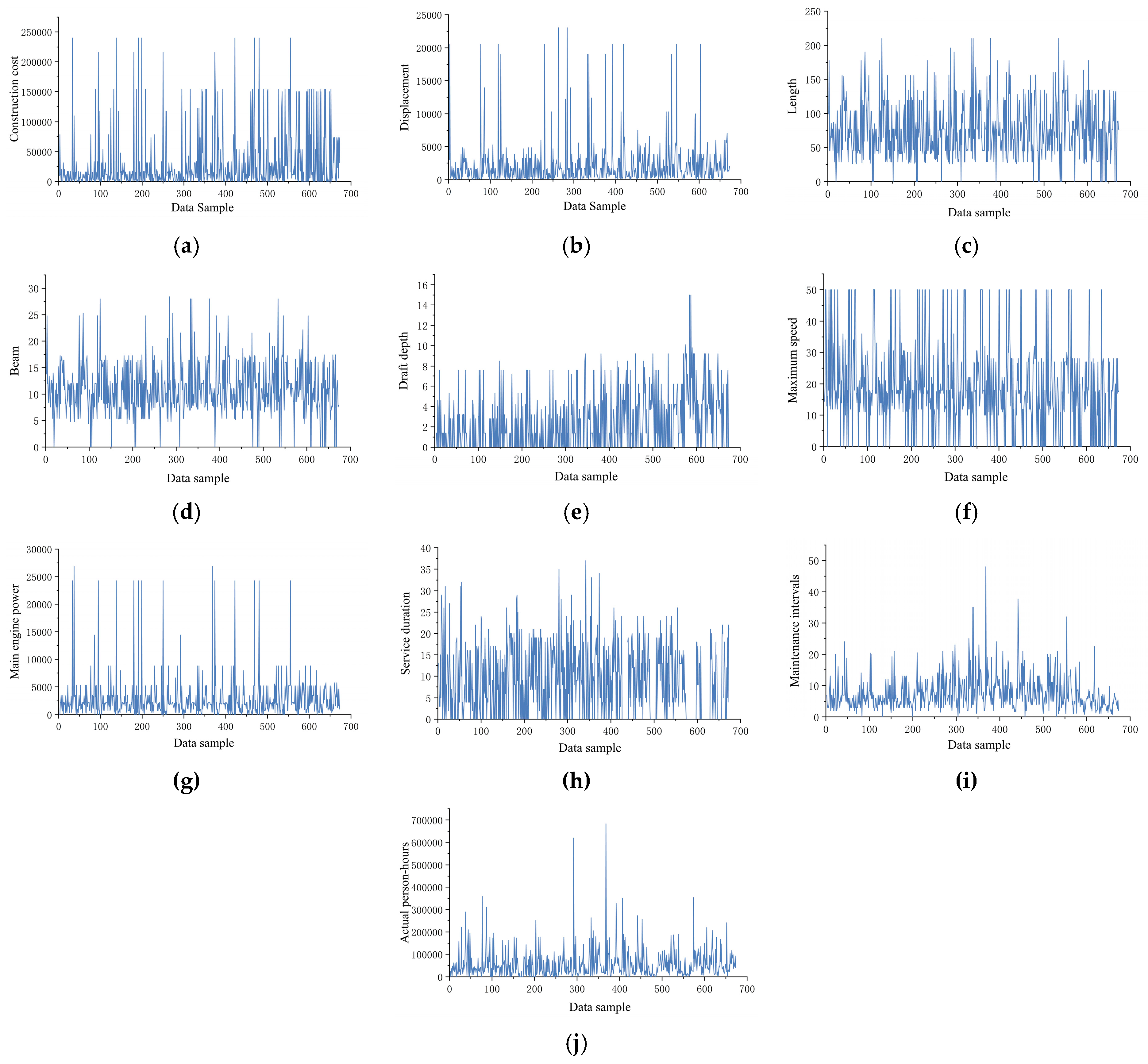
- Step 4. Imputation Effectiveness and Limitations. Empirical analysis reveals that when fields with missing rates exceeding 25% (e.g., draft depth) and their correlated variables exhibit concurrent data gaps, the loss of nonlinear correlations among features compromises model inference capabilities. For imputing maintenance records of large vessels with a displacement of >20,000 tons, prediction errors significantly increase due to insufficient abnormal-condition samples, necessitating secondary validation. Post-imputation data distributions across all variables are visualized in Figure 13.
4.3. Discussion and Analysis
4.3.1. Comparative Analysis of Outlier Mining Algorithms
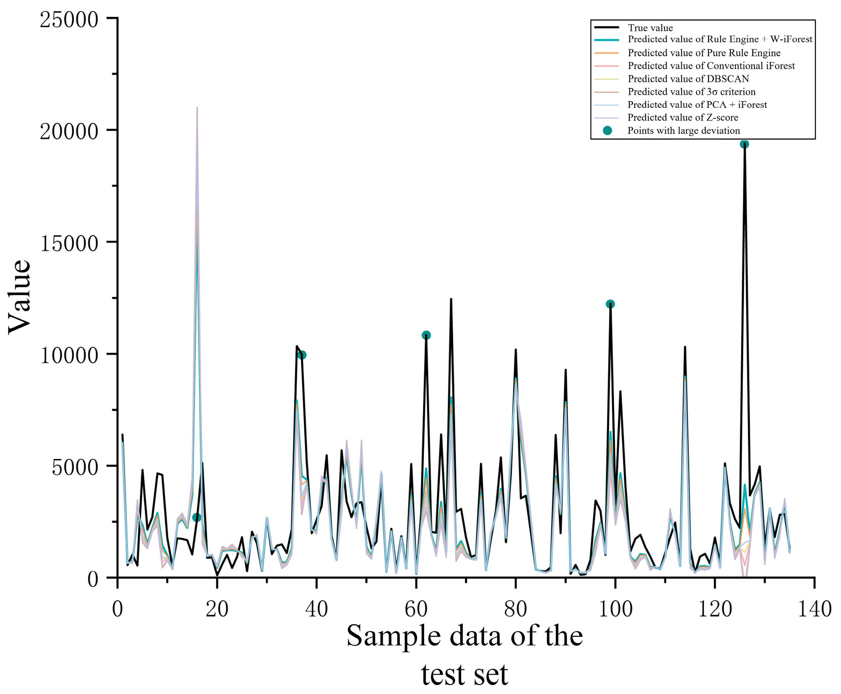
4.3.2. Comparative Analysis of Missing Value Imputation Algorithms
4.3.3. Comparative Analysis of Data-Cleansing Algorithms
4.3.4. Ablation Study
5. Conclusions
Author Contributions
Funding
Data Availability Statement
Conflicts of Interest
Abbreviations
| W-iForest | Feature-Weighted Isolation Forest Algorithm |
| GA-ACO-RF | Genetic Algorithm–Ant Colony Optimization Collaborative Random Forest |
| RPD | Relative Percentage Difference |
| iForest | Isolation Forest |
| LOF | Local Outlier Factor |
| GMM | Gaussian Mixture Model |
| GBDT | Gradient Boosting Decision Tree |
| GA | Genetic Algorithms |
| ACO | Ant Colony Optimization |
| RF | Random Forest |
| IQR | Interquartile Range |
| GNNs | Graph Neural Networks |
| TSR | Tip-speed Ratio |
| SVM | Support Vector Machines |
| LSTM | Long Short-Term Memory |
| AEs | Autoencoders |
| SDAEs | Stacked Denoising Autoencoders |
| MI | Multiple Imputation |
| MCMC | Markov Chain Monte Carlo |
| MCM | Matrix Completion Methods |
| MAR | Missing at Random |
| MNAR | Missing Not at Random |
| GANs | Generative Adversarial Networks |
| VAEs | Variational Autoencoders |
| PCA | Principal Component Analysis |
| t-SNE | t-Distributed Stochastic Neighbor Embedding |
| CART | Classification and Regression Tree |
| PPI | Producer Price Index |
| MICE | Multiple Imputation by Chained Equations |
| CDF | Cumulative Distribution Function |
| AD | Anomaly Detection |
Appendix A
| Algorithm A1. iForest |
| Inputs:—feature weight matrix |
| Output: a set ofiTrees |
| 1: initialize Forest |
| 2: set height limit |
| 3: for to do |
| 4: ←sample |
| 5. Forest←ForestiTree |
| 6. end for |
| 7. return Forest |
| Algorithm A2. iTree |
| Inputs:—height limit |
| Output: an iTree |
| 1: if or then |
| 2: return LeafNode |
| 3: else |
| 4: # select feature based on weight distribution |
| 5. randomly select a feature from dimensions with probability distribution |
| 6. # randomly select split point within the range of feature |
| 7. uniformly sample between |
| 8. # split data into left/right subtrees |
| 9. |
| 10. |
| 11. return InternalNode |
| 12. end if |
| Algorithm A3. PathLength |
| Inputs:—an iTree |
| Output:—path length |
| 1: |
| 2: while tree is not a LeafNode |
| 3. . SplitFeature |
| 4. . SplitValue |
| 5. if |
| 6. |
| 7. else |
| 8. |
| 9. |
| 10. # adjust path length using harmonic number (Equation (2) in the document) |
| 11. |
| 12. return |
| 13. end if |
| Algorithm A4. GA-ACO-RF Imputation |
| Inputs: |
| features) |
| : RF hyperparameter search space (n_estimators, max_depth, ...) |
| genetic algorithm parameters (population size, generations, crossover rate, mutation rate |
| ant colony parameters (ants, pheromone decay |
| Output: |
| : imputed complete dataset |
| optimized RF hyperparameters |
| 1: initialization |
| 2: encode RF hyperparameters into chromosome structures (real-value encoding) |
| 3: generate initial GA population via random sampling |
| 4: GA Global Optimization Phase |
| 5. for to do |
| 6. fitness evaluation: |
| 7. for each chromosome in : |
| 8. train RF model with k-fold cross-validation |
| 9. compute fitness as on validation set |
| 10. selection: |
| 11. perform roulette wheel selection to retain elite individuals |
| 12. crossover: |
| 13. apply single-point crossover to generate offspring (probability ) |
| 14. Mutation: 15. introduce Gaussian noise to chromosomes (probability ) |
| 16. ACO Local Refinement Phase: |
| 17. map hyperparameter space to ACO path nodes |
| 18. initialize pheromone proportional to GA fitness values |
| 19. for each ant to do |
| 20. Path Construction: |
| 21. select hyperparameters via probabilistic rule (Equation (18)) |
| 22. Pheromone Update: |
| 23. update based on imputation performance (Equation (15)) |
| 24. Adaptive Reset: |
| 25. periodically reinitialize stagnant paths to avoid local optima |
| 26. Imputation with Optimized RF: |
| 27. extract optimal hyperparameters from ACO |
| 28. train GA-ACO-RF model |
| 29. for each missing feature in do |
| 30. set as target, train RF regressor on complete features |
| 31. predict missing values and update |
| 32. iterate until convergence (max iterations or error threshold) |
| 33. return , |
Appendix B

| Sample Table for Ship-Maintenance-Cost Data Collection | |||
|---|---|---|---|
| (1) Basic Vessel Info | |||
| Vessel Type | XXX | Vessel Model | XXX |
| Commissioning Date | XXX | Vessel Age (Years) | XXX |
| (2) Vessel Attributes | |||
| Construction Cost (CNY 10,000) | XXX | Displacement (Ton) | XXX |
| Length (m) | XXX | Beam (m) | XXX |
| Draft Depth (m) | XXX | Maximum Speed (Knots) | XXX |
| Propulsion System Type | XXX | Main Engine Power (KW) | XXX |
| (3) Contractor Details | |||
| Contractor Name | XXX | Frontline Technicians Count | XXX |
| Frontline Workforce Ratio (%) | XXX | Total Task Hours (Hours) | XXX |
| Fixed Assets Original Value (CNY 10,000 ) | XXX | Operating Revenue (CNY 10,000) | XXX |
| Operating Profit (CNY 10,000) | XXX | - | - |
| (4) Maintenance Costs | |||
| Direct Materials Cost (CNY 10,000) | XXX | Direct Labor Cost (CNY 10,000) | XXX |
| Manufacturing Overhead (CNY 10,000) | XXX | Specialized Expenses (CNY 10,000) | XXX |
| Period Costs (CNY 10,000) | XXX | Total Maintenance Cost (CNY 10,000) | XXX |
Appendix C
| Symbol | Meaning | Symbol | Meaning |
|---|---|---|---|
| Displacement (ton) | Expert experience weight | ||
| Length of ship (m) | Experience correction coefficient | ||
| Breadth of ship (m) | Standardized path length of iForest | ||
| Draft of ship (m) | Harmonic number of iForest | ||
| Main engine power (kW) | Euler’s constant | ||
| Maximum speed (kn) | Anomaly score of iForest | ||
| Ship type coefficient | Expected value of path length of sample in multiple iTrees | ||
| , | Minimum and maximum values of length–breadth ratio | Squared error loss function of CART algorithm | |
| Total maintenance person-hours (h) | , | Number of samples in left and right subsets after RF splitting | |
| Maintenance days | , | Means of left and right subsets after RF splitting | |
| Number of maintenance participants | , | Crossover rate and mutation rate of GA | |
| Actual replacement cycle | Maximum number of iterations of GA | ||
| Design life | Pheromone concentration of node j in ACO | ||
| Maintenance cost | Ant colony size of ACO | ||
| Construction cost | Pheromone evaporation coefficient of ACO | ||
| Safety coefficient for spare parts replacement | Pheromone increment of the k-th ant on path j | ||
| Damage coefficient of maintenance cost | Heuristic information of path i→j | ||
| Service life (years) | Transition probability from node i to node j for ant k at time t | ||
| Weight of rule i | Set of unexplored nodes accessible to ant k at node i | ||
| Weight of feature i | , | Weights of pheromone and heuristic factors in ACO | |
| Trigger frequency of rule |
References
- Golovan, A.; Mateichyk, V.; Gritsuk, I.; Lavrov, A.; Smieszek, M.; Honcharuk, I.; Volska, O. Enhancing Information Exchange in Ship Maintenance through Digital Twins and IoT: A Comprehensive Framework. Computers 2024, 13, 261. [Google Scholar] [CrossRef]
- Zhang, K.; Xi, P.; Liang, X.; Li, X. Decision-making Method and Application of Ship Maintenance Resource Allocation Based on ε-EGA Multi-criteria Adjustment. Oper. Res. Manag. Sci. 2023, 32, 53–60. [Google Scholar] [CrossRef]
- Ji, R.; Hou, H.; Sheng, G.; Zhang, L.; Shu, B.; Jiang, X. Data Quality Improvement Method for Power Equipment Condition Based on Stacked Denoising Autoencoders Improved by Particle Swarm Optimization. J. Shanghai Jiao Tong Univ. 2024. [Google Scholar] [CrossRef]
- Wang, S.; Li, B.; Li, G.; Yao, B.; Wu, J. Short-term wind power prediction based on multidimensional data cleaning and feature reconfiguration. Appl. Energy 2021, 292, 116851. [Google Scholar] [CrossRef]
- Wang, D.; Li, S.; Fu, X. Short-Term Power Load Forecasting Based on Secondary Cleaning and CNN-BILSTM-Attention. Energies 2024, 17, 4142. [Google Scholar] [CrossRef]
- Shen, X.; Fu, X.; Zhou, C. A Combined Algorithm for Cleaning Abnormal Data of Wind Turbine Power Curve Based on Change Point Grouping Algorithm and Quartile Algorithm. IEEE Trans. Sustain. Energy 2019, 10, 46–54. [Google Scholar] [CrossRef]
- Brandis, V.A.; Menges, D.; Rasheed, A. Multi-Target Tracking for Autonomous Surface Vessels Using LiDAR and AIS Data Integration. Appl. Ocean Res. 2025, 154, 104348. [Google Scholar] [CrossRef]
- Deng, Y.; Li, Y.; Zhu, H.; Fan, S. Displacement Values Calculation Method for Ship Multi-Support Shafting Based on Transfer Learning. J. Mar. Sci. Eng. 2024, 12, 36. [Google Scholar] [CrossRef]
- Yao, Y.; Zhang, X.; Cui, W. A LOF-IDW based data cleaning method for quality assessment in intelligent com-paction of soils. Transp. Geotech. 2023, 42, 101101. [Google Scholar] [CrossRef]
- Zhu, H.; Zhang, X.; Wu, J.; Hu, S.; Wang, Y. A novel solar irradiance calculation method for distributed photo-voltaic power plants based on K-dimension tree and combined CNN-LSTM method. Comput. Electr. Eng. 2025, 122, 109990. [Google Scholar] [CrossRef]
- Song, C.; Cui, J.; Cui, Y.; Zhang, S.; Wu, C.; Qin, X.; Wu, Q.; Chi, S.; Yang, M.; Liu, J.; et al. Inte-grated STL-DBSCAN Algorithm for Online Hydrological and Water Quality Monitoring Data Cleaning. Environ. Ment. Model. Softw. 2025, 183, 106262. [Google Scholar] [CrossRef]
- Han, B.; Xie, H.; Shan, Y.; Liu, R.; Cao, S. Characteristic Curve Fitting Method of Wind Speed and Wind Tur-bine Output Based on Abnormal Data Cleaning. J. Phys. Conf. Ser. 2022, 2185, 012085. [Google Scholar] [CrossRef]
- Liu, Y.; Liu, D.; Zhang, Y.; Wu, M. Configuration Type Identification Integrating Multi-Granularity Code Features and Isolation Forest Algorithm. Comput. Eng. Appl. 2024. Available online: https://link.cnki.net/urlid/11.2127.TP.20241120.1628.006 (accessed on 16 May 2025).
- Shen, L.; He, X.; Liu, M.; Qin, R.; Guo, C.; Meng, X.; Duan, R. A Flexible Ensemble Algorithm for Big Data Cleaning of PMUs. Front. Energy Res. 2021, 9, 695057. [Google Scholar] [CrossRef]
- Si, S.; Xiong, W.; Che, X. Data Quality Analysis and Improvement: A Case Study of a Bus Transportation System. Appl. Sci. 2023, 13, 11020. [Google Scholar] [CrossRef]
- Yin, Q.; Zhao, G. A Study on Data Cleaning for Energy Efficiency of Ships. J. Transp. Inf. Saf. 2017, 35, 68–73. [Google Scholar] [CrossRef]
- Feng, Z.; Zhu, S.; Zhao, Z.; Sun, M.; Dong, M.; Song, D. Comparative Study on Detection Methods of Wind Power Abnormal Data. Adv. Technol. Electr. Eng. Energy 2021, 40, 55–61. [Google Scholar] [CrossRef]
- Lai, G.; Liao, L.; Zhang, L.; Li, T. Wind Speed Power Data Cleaning Method for Wind Turbines Based on Fan Characteristics and Isolated Forests. J. Phys. Conf. Ser. 2023, 2427, 12001. [Google Scholar] [CrossRef]
- Li, L.; Liang, Y.; Lin, N.; Yan, J.; Meng, H.; Liu, Y. Data Cleaning Method Considering Temporal and Spatial Cor-relation for Measured Wind Speed of Wind Turbines. Acta Energiae Solaris Sin. 2024, 45, 461–469. [Google Scholar] [CrossRef]
- Huang, G.; Long, Z.; Zhu, Z.; Cheng, W. Monitoring Data Cleaning for Water Distribution System Based on Support Vector Machine. Water Wastewater Eng. 2022, 14, 124–129. [Google Scholar] [CrossRef]
- Mei, Y.; Li, X.; Hu, Z.; Yao, H.; Liu, D. Identification and Cleaning of Wind Power Data Methods Based on Control Principle of Wind Turbine Generator System. J. Chin. Soc. Power Eng. 2021, 41, 316–322, 329. [Google Scholar] [CrossRef]
- Xu, B. Parameter Correlation Based Parameter Abnormal Point Cleaning Method for Power Station. Autom. Electr. Power Syst. 2020, 44, 142–147. [Google Scholar] [CrossRef]
- Cui, X.; Lin, H.; An, N.; Wang, R. Ship Navigation Data Recognition Based on LOF-FCM Algorithm. Ship Eng. 2024, 46, 488–493. [Google Scholar] [CrossRef]
- Meng, L.; Zhang, R.; Li, X.; Xi, Y. Cleaning Abnormal Status Data of Substation Equipment Based on Machine Learning. Proc. CSU-EPSA 2021, 33, 8. [Google Scholar] [CrossRef]
- Liu, J.; Zhang, A.; Huang, Z.; Huang, D.; Chen, X. Dimension Reduction Optimization Analysis of CSE-CIC-IDS2018 Intrusion Detection Dataset Based on Machine Learning. Fire Control Command Control 2021, 46, 8. [Google Scholar] [CrossRef]
- Han, H.; Lu, S.; Wu, X.; Qiao, J. Abnormal Data Cleaning Method for Municipal Wastewater Treatment Based on Improved Support Vector Machine. J. Beijing Univ. Technol. 2021, 47, 1011–1020. [Google Scholar] [CrossRef]
- Yang, H.; Tang, J.; Shao, W.; Liu, B.; Chen, R. Wind Power Data Cleaning Method Based on Rule Base and PRRL Model. Acta Energiae Solaris Sin. 2024, 45, 416–425. [Google Scholar] [CrossRef]
- Gu, J.; Zhao, J.; Zhang, X.; Cheng, T.; Zhou, B.; Jiang, L. Research Review and Prospect of Data Cleaning for Multi-Parameter Monitoring Data of Power Equipment. High Volt. Eng. 2024, 50, 3403–3420. [Google Scholar] [CrossRef]
- Côté, P.O.; Nikanjam, A.; Ahmed, N.; Humeniuk, D.; Khomh, F. Data Cleaning and Machine Learning: A Systematic Literature Review. Autom. Softw. Eng. 2024, 31, 54. [Google Scholar] [CrossRef]
- Xia, Y.; Xia, H.; Feng, X. Research on SCADA Data Cleaning Method Based on Wind Power Curve. Renew. Energy Resour. 2022, 40, 1499–1504. [Google Scholar] [CrossRef]
- Xu, X.; Wang, Z.; Wang, H. Turbine Data Cleaning Based on Deep LSTM. Therm. Power Gener. 2023, 52, 179–187. [Google Scholar] [CrossRef]
- Zhao, D.; Shen, Z.; Song, Z.; Xie, L.; Liu, B. Mine Airflow Speed Sensor Data Cleaning Model for Intelligent Ventilation. China Saf. Sci. J. 2023, 33, 56–62. [Google Scholar] [CrossRef]
- Peng, B.; Li, Y.; Gong, X. Improved K-Means Photovoltaic Energy Data Cleaning Method Based on Autoencoder. Comput. Sci. 2024, 51, 230700070-5. [Google Scholar] [CrossRef]
- Liu, X.; Zhang, W.-J.; Shi, Q.; Zhou, L. Operation Parameters Optimization of Blast Furnaces Based on Data Mining and Cleaning. J. Northeast. Univ. Nat. Sci. 2020, 41, 1153–1160. [Google Scholar] [CrossRef]
- Zhu, Y.; Liang, W.; Wang, Y. Research on Data Cleaning and Fusion in Distribution Power Grid Based on Time Series Technology. Power Syst. Technol. 2021, 45, 2839–2846. [Google Scholar] [CrossRef]
- Wang, H.; Chen, Y.; Fan, T.; Xie, X.; Ma, D. On Line Cleaning and Repairing Method of Photovoltaic System Data Acquisition. Acta Energiae Solaris Sin. 2022, 43, 57–65. [Google Scholar] [CrossRef]
- Chen, Z.; Jiang, P.; Liu, J.; Zheng, S.; Shan, Z.; Li, Z. An Adaptive Data Cleaning Framework: A Case Study of the Water Quality Monitoring System in China. Hydrol. Sci. J. 2022, 67, 1114–1129. [Google Scholar] [CrossRef]
- Jäger, S.; Allhorn, A.; Bießmann, F. A Benchmark for Data Imputation Methods. Front. Big Data 2021, 4, 693674. [Google Scholar] [CrossRef]
- Zhang, X.; Sun, X.; Xia, L.; Tao, S.; Xiang, S. A Matrix Completion Method for Imputing Missing Values of Process Data. Processes 2024, 12, 659. [Google Scholar] [CrossRef]
- Liu, Q.; Zhong, Y.; Lin, C.; Li, T.; Yang, C.; Fu, Z.; Li, X. Electricity Consumption Data Cleansing and Imputation Based on Robust Nonnegative Matrix Factorization. Power Syst. Technol. 2024, 48, 2103–2112. [Google Scholar] [CrossRef]
- Maharana, K.; Mondal, S.; Nemade, B. A Review: Data Pre-Processing and Data Augmentation Techniques. Glob. Transit. Proc. 2022, 3, 91–99. [Google Scholar] [CrossRef]
- Mohammed, A.F.Y.; Sultan, S.M.; Lee, J.; Lim, S. Deep-Reinforcement-Learning-Based IoT Sensor Data Cleaning Framework for Enhanced Data Analytics. Sensors 2023, 23, 1791. [Google Scholar] [CrossRef] [PubMed]
- Clemente, D.; Rosa-Santos, P.; Taveira-Pinto, F. Numerical Developments on the E-Motions Wave Energy Converter: Hull Design, Power Take-Off Tuning and Mooring System Configuration. Ocean. Eng. 2023, 280, 114596. [Google Scholar] [CrossRef]
- Song, M.; Shi, Q.; Zhang, F.; Wang, Y.; Li, L. Assessment of Rush Repair Capacity of Wartime Equipment Re-pair Institutions. J. Ordnance Equip. Eng. 2020, 41, 241–244. [Google Scholar] [CrossRef]
- Ge, C.; Gao, Y.; Miao, X.; Yao, B.; Wang, H. A Hybrid Data Cleaning Framework Using Markov Logic Net-works (Extended Abstract). In Proceedings of the 2021 IEEE 37th International Conference on Data Engineering (ICDE), Chania, Greece, 19–22 April 2021; pp. 2344–2345. [Google Scholar] [CrossRef]
- Huang, G.; Zhao, X.; Lu, Q. Research on multi-source VOCs data cleaning method based on KPCA-IF-WRF model. J. Saf. Environ. 2022, 22, 3412–3423. [Google Scholar] [CrossRef]
- Li, X.; Liu, M.; Wang, K.; Liu, Z.; Li, G. Data Cleaning Method for the Process of Acid Production with Flue Gas Based on Improved Random Forest. Chin. J. Chem. Eng. 2023, 59, 72–84. [Google Scholar] [CrossRef]
- Li, M.; Su, M.; Zhang, B.; Yue, Y.; Wang, J.; Deng, Y. Research on a DBSCAN-IForest Optimisation-Based Anomaly Detection Algorithm for Underwater Terrain Data. Water 2025, 17, 626. [Google Scholar] [CrossRef]
- Saneep, K.; Sundareswaran, K.; Nayak, P.S.R.; Puthusserry, G.V. State of Charge Estimation of Lithium-Ion Batteries Using PSO Optimized Random Forest Algorithm and Performance Analysis. J. Energy Storage 2025, 114, 115879. [Google Scholar] [CrossRef]
- Wang, C.; Huang, Z.; He, C.; Lin, X.; Li, C.; Huang, J. Research on Remaining Useful Life Prediction Method for Lithium-Ion Battery Based on Improved GA-ACO-BPNN Optimization Algorithm. Sustain. Energy Technol. Assess. 2025, 73, 104142. [Google Scholar] [CrossRef]
- Zheng, Y.; Lv, X.; Qian, L.; Liu, X. An Optimal BP Neural Network Track Prediction Method Based on a GA–ACO Hybrid Algorithm. J. Mar. Sci. Eng. 2022, 10, 1399. [Google Scholar] [CrossRef]
- He, G.; Du, Y.; Liang, Q.; Zhou, Z.; Shu, L. Modeling and Optimization Method of Laser Cladding Based on GA-ACO-RFR and GNSGA-II. Int. J. Precis. Eng. Manuf.-Green Technol. 2023, 10, 1207–1222. [Google Scholar] [CrossRef]
- Li, T.; Deng, L.; Mo, B.; Shi, F. Prediction of Cracks and Optimization of Process Parameters in Laser Cladding of Ni60 Based on GA-ACO-RFA. China Mech. Eng. 2024. Available online: https://link.cnki.net/urlid/42.1294.th.20240708.1823.012 (accessed on 20 May 2025).


| ID | Vessel Type | Displacement (tons) | Length (m) | Max Speed (knots) | Prime Mover Type | Power Rating (kW) |
|---|---|---|---|---|---|---|
| 1 | 7500 | 152 | 32 | Gas Turbine | 70,000 | |
| 2 | 7500 | 152 | 32 | Gas Turbine | 70,000 | |
| 3 | 32,000 | 85 | 18 | Diesel Engine | 5000 | |
| 4 | 40,000 | 220 | - | - | 30,000 | |
| 5 | 15,000 | 180 | 28 | Steam Turbine | 200,000 | |
| 6 | - | 200 | - | Steam Turbine | 120,000 | |
| 7 | 3800 | - | 24 | Diesel Engine | 12,000 | |
| 8 | 8000 | 158 | 55 | Gas Turbine | 75,000 |
| Method | Representative Algorithms | Advantages | Limitations | Applicable Scenarios |
|---|---|---|---|---|
| Statistical Analysis | criterion, Box plot | Simple computation, real-time capability | Relies on distribution assumptions, ignores correlations | Univariate low-dimensional data |
| Density Clustering | DBSCAN, LOF | Identifies local anomalies | Parameter sensitivity, high computational complexity | Complex distribution data |
| Machine Learning | iForest, SVM | Automation, multi-source adaptability | Requires labeled data or parameter tuning | Multi-dimensional structured data |
| Deep Learning | LSTM, GNN | High-order feature extraction | High computational cost, poor interpretability | Temporal/image/graph-structured data |
| Method | Typical Algorithms | Advantages | Limitations | Applicable Scenarios |
|---|---|---|---|---|
| Traditional | Mean, Spline Interpolation | Simple implementation, fast computation | Ignores variable correlations | Low missing rates, univariate data |
| Statistical Models | MI, MCM | Preserves statistical properties | Relies on distribution assumptions | Structured data, MAR mechanisms |
| Machine Learning | RF, GANs | High accuracy, nonlinear adaptability | High computational resource demands | High-dimensional data, MNAR mechanisms |
| Rule Name | Mathematical Expression | Symbol Definitions | Physical Principle | Tolerance |
|---|---|---|---|---|
| Displacement Verification | : Displacement (ton) | Archimedes’ principle | ±2% Hull form tolerance | |
| : Length (m) | ||||
| : Beam (m) | ||||
| : Draft (m) | ||||
| Speed–Power Relationship | : Main engine power (KW) | Hydrodynamic resistance model | Power reserve ≥ 15% | |
| : Max speed (kn) | ||||
| : Hull coefficient | ||||
| Length–Beam Ratio Limit | ratio | Stability–speed balance equation | Elastic range ±0.2 | |
| ratio |
| Rule Name | Mathematical Expression | Symbol Definitions | Business Logic |
|---|---|---|---|
| Person-hour Efficiency | : Total person-hours (h) | ||
| : Maintenance days | |||
| : Technicians assigned | |||
| Component Replacement | : Safety factor | ||
| Maintenance-Cost Correlation | : Damage coefficient | ||
| : Service years |
| Variable | Feature Weight | Variable | Feature Weight | Variable | Feature Weight | Variable | Feature Weight |
|---|---|---|---|---|---|---|---|
| Construction Cost | 0.0065 | Displacement | 0.1360 | Length | 0.1446 | Beam | 0.1446 |
| Draft Depth | 0.1360 | Maximum Speed | 0.1506 | Main Engine Power | 0.1506 | Service Years | 0.0065 |
| Maintenance Cycle | 0.0394 | Personnel Count | 0.0394 | Actual Person-Hours | 0.0394 | Total Maintenance Cost | 0.0065 |
| Parameter Name | Symbol | Value |
|---|---|---|
| GA Algorithm | ||
| Crossover Probability | 0.7 | |
| Mutation Probability | 0.2 | |
| Maximum Iterations | 50 | |
| ACO Algorithm | ||
| Ant Colony Size | 20 | |
| Pheromone Evaporation Coefficient | 0.5 | |
| Pheromone Weight | 1 | |
| Heuristic Factor Weight | 2 | |
| RF Algorithm | ||
| Number of Decision Trees | n_estimators | 191 |
| Maximum Tree Depth | max_depth | 11 |
| Minimum Samples for Node Split | min_samples_split | 2 |
| Minimum Samples per Leaf Node | min_samples_leaf | 1 |
| Method | Number of Detected Anomalies | Number of Detected Anomalies (%) | Recall (%) | F1-Score (%) | False Positive Rate (%) |
|---|---|---|---|---|---|
| Rule Engine + W-iForest | 107 | 92.5 | 95.3 | 93.8 | 7.5 |
| Pure Rule Engine | 40 | 85.0 | 60.0 | 70.6 | 15.0 |
| Conventional iForest | 89 | 73.0 | 82.1 | 77.3 | 27.0 |
| DBSCAN | 63 | 68.2 | 55.6 | 61.3 | 31.8 |
| Criterion | 52 | 65.4 | 48.1 | 55.4 | 34.6 |
| PCA-iForest | 78 | 71.8 | 74.4 | 73.1 | 28.2 |
| Z-score | 45 | 62.2 | 42.2 | 50.0 | 37.8 |
| Method | RMSE | MAE | MAPE | R2 |
|---|---|---|---|---|
| Rule Engine + W-iForest | 2253.5 | 1068.7 | 41.1% | 0.4233 |
| Pure Rule Engine | 2380.2 | 1145.3 | 45.2% | 0.3865 |
| Conventional iForest | 2780.4 | 1320.7 | 52.3% | 0.2841 |
| DBSCAN | 2651.0 | 1280.5 | 49.8% | 0.3157 |
| Criterion | 2950.1 | 1410.9 | 55.1% | 0.2345 |
| PCA-iForest | 2590.6 | 1250.3 | 48.9% | 0.3278 |
| Z-score | 2870.9 | 1380.5 | 53.7% | 0.2562 |
| Method | RMSE | MAE | MAPE | R2 |
|---|---|---|---|---|
| Mean imputation | 2350.1 | 1050.6 | 42.7% | 0.4102 |
| KNN imputation | 2100.8 | 890.3 | 35.9% | 0.5321 |
| MICE | 1985.4 | 810.2 | 32.1% | 0.5987 |
| Conventional RF imputation | 1850.2 | 750.5 | 30.8% | 0.6320 |
| GA-RF imputation | 1780.9 | 730.1 | 29.5% | 0.6543 |
| ACO-RF imputation | 1735.6 | 715.4 | 29.0% | 0.6638 |
| GA-ACO-RF imputation | 1667.3 | 697.9 | 28.3% | 0.6714 |
| Method | RMSE | MAE | MAPE | R2 |
|---|---|---|---|---|
| Hybrid Algorithm | 1667.3 | 697.9 | 28.3% | 0.6714 |
| Conventional iForest | 2223.1 | 902.6 | 35.7% | 0.5321 |
| Conventional RF | 2058.4 | 834.2 | 32.1% | 0.5983 |
| K-means Algorithm | 2198.5 | 891.4 | 36.2% | 0.5438 |
| Mutual Information Algorithm | 2310.7 | 945.8 | 38.5% | 0.4876 |
| Dateset | RMSE | RMSE | MAE | MAE | R2 | R2 |
|---|---|---|---|---|---|---|
| Base | 3371.1 | 2334.0 | 0.2931 | |||
| Base+AD | 2253.5 | −33.2% | 1068.7 | −54.2% | 0.4233 | +44% |
| Full | 1667.3 | −26.0% | 697.9 | −34.7% | 0.6714 | +59% |
Disclaimer/Publisher’s Note: The statements, opinions and data contained in all publications are solely those of the individual author(s) and contributor(s) and not of MDPI and/or the editor(s). MDPI and/or the editor(s) disclaim responsibility for any injury to people or property resulting from any ideas, methods, instructions or products referred to in the content. |
© 2025 by the authors. Licensee MDPI, Basel, Switzerland. This article is an open access article distributed under the terms and conditions of the Creative Commons Attribution (CC BY) license (https://creativecommons.org/licenses/by/4.0/).
Share and Cite
Zhu, C.; Sun, S.; Xie, L.; Wang, Y.; Li, K.; Li, J. A Hybrid Data-Cleansing Framework Integrating Physical Constraints and Anomaly Detection for Ship Maintenance-Cost Prediction via Enhanced Ant Colony–Random Forest Optimization. Processes 2025, 13, 2035. https://doi.org/10.3390/pr13072035
Zhu C, Sun S, Xie L, Wang Y, Li K, Li J. A Hybrid Data-Cleansing Framework Integrating Physical Constraints and Anomaly Detection for Ship Maintenance-Cost Prediction via Enhanced Ant Colony–Random Forest Optimization. Processes. 2025; 13(7):2035. https://doi.org/10.3390/pr13072035
Chicago/Turabian StyleZhu, Chen, Shengxiang Sun, Li Xie, Yang Wang, Kai Li, and Jing Li. 2025. "A Hybrid Data-Cleansing Framework Integrating Physical Constraints and Anomaly Detection for Ship Maintenance-Cost Prediction via Enhanced Ant Colony–Random Forest Optimization" Processes 13, no. 7: 2035. https://doi.org/10.3390/pr13072035
APA StyleZhu, C., Sun, S., Xie, L., Wang, Y., Li, K., & Li, J. (2025). A Hybrid Data-Cleansing Framework Integrating Physical Constraints and Anomaly Detection for Ship Maintenance-Cost Prediction via Enhanced Ant Colony–Random Forest Optimization. Processes, 13(7), 2035. https://doi.org/10.3390/pr13072035