Abstract
Traditional data-driven approaches to lithium battery state of health (SOH) estimation face the challenges of difficult feature extraction, insufficient prediction accuracy and weak generalization. To address these issues, this study proposes a novel prediction framework with transfer learning-based linear regression (LR) and a convolutional neural network (CNN) under limited data. In this framework, first, variable inertia weight-based improved particle swarm optimization for variational mode decomposition (VIW-PSO-VMD) is proposed to mitigate the volatility of the “capacity resurgence point” and extract its time-series features. Then, the T-Pearson correlation analysis is introduced to comprehensively analyze the correlations between multivariate features and lithium battery SOH data and accurately extract strongly correlated features to learn the common features of lithium batteries. On this basis, a combination model is proposed, applying LR to extract the trend features and combining them with the multivariate strongly correlated features via a CNN. Transfer learning based on temporal feature analysis is used to improve the cross-domain learning capabilities of the model. We conduct case studies on a NASA dataset and the University of Maryland dataset. The results show that the proposed method is effective in improving the lithium battery SOH estimation accuracy under limited data.
1. Introduction
With the rapid development of global renewable energy, lithium batteries have become the main solution to the problem of the grid-connected stability of renewable energy due to their high energy density, long cycle life, and relatively low self-discharge rate [1]. The reason is that renewable energy sources such as solar energy and wind energy are unstable and intermittent during generation, which makes it difficult to apply these valuable forms of energy continuously and stably. To tackle this issue, the employment of energy storage systems combined with renewable energy may greatly improve the utilization rate and stability of renewable energy [2,3]. However, with an increase in the number of uses, lithium batteries will exhibit the battery degradation phenomenon, resulting in a decline in battery capacity, shortening the service life, etc. [4], which seriously affects the charging and discharging efficiency of the battery. Thus, the accurate estimation of the performance of lithium batteries is key to realize the safe and stable consumption of renewable energy [5].
The state of health (SOH) of lithium batteries is an important indicator in evaluating their performance. In existing research, the prediction of the lithium battery SOH is mainly categorized into direct measurement, model-based prediction, and data-driven prediction methods [6]. The direct measurement method and the model-based prediction method have high professional requirements and require sufficient knowledge reserves, while the battery’s response in the charging and discharging process is complex and involves more parameters, which makes the model’s construction more difficult [7,8]. Compared with the above two methods, the data-driven method is based on historical data, learns the hidden features of the data through machine learning algorithms such as neural networks, and realizes the prediction of the SOH based on the learned features.
In the data-driven prediction approach, researchers have searched for the accurate mapping relationship between the features and SOH through feature processing, using recurrent neural networks [9], machine learning algorithms [10], Gaussian regression [11], etc. Wen J et al. predicted the SOH of lithium batteries via incremental capacity curves and analyzed them in combination with backpropagation (BP) neural networks, but BP neural networks are unable to learn time-series features, and it is difficult to accurately characterize the trend of the SOH through a single feature [12]. Xia F et al. analyzed the correlations between different feature curves and the SOH via Pearson correlation analysis (PCA). They then used improved particle swarm optimization (PSO) to optimize the network parameters of a bidirectional gated recurrent unit and trained and predicted the SOH based on the model. However, tripartite competition mechanism PSO (TCMPSO) reduces the speed of optimization, which makes the model less efficient for prediction in practical applications [13]. Zhao D et al. proposed a prediction method integrating a neural network and physical model and constructed a hybrid model combining a temporal convolutional network and bidirectional long short-term memory network to predict the SOH of lithium batteries [14]. A large number of researchers have achieved better performance in estimating the SOH of lithium batteries by analyzing the correlations between the physical features and SOH and using neural networks to extract the mapping relationships between the strongly correlated features and SOH [15,16,17]. However, in the process of practical application, energy storage batteries are limited by factors such as the application scenario, and there is the phenomenon of low data volumes, in which case the neural network will have problems such as underfitting and will not be able to accurately learn the mapping relationship between the features and SOH.
“Capacity regeneration” is another reason that it is difficult to realize the accurate estimation of lithium batteries. Due to the versatility of charging and discharging strategies, the SOH of lithium batteries presents a fluctuating downward trend with strong volatility at a certain stage. To address this problem, existing studies have proposed the use of decomposition algorithms [18]. The purpose of decomposing the raw SOH data includes mitigating the degree of volatility and removing volatile information. After the mitigation process, the “capacity regeneration” information is still retained in the dataset, and the data have a high degree of realism; after the elimination process, the “capacity regeneration” is rejected as anomalous data. The mitigation process enables the neural network to learn the historical “capacity regeneration” information; the elimination process can extract the core trend of the SOH. Fu J et al. used variational mode decomposition (VMD) to mitigate the effects of “capacity regeneration” and then reconstructed the components based on the entropy of the alignment [19]. Yuan Z et al. eliminated “capacity regeneration” and noise signals by VMD and then used a convolutional neural network and Transformer to estimate the SOH [20]. Although the above research mitigated the effects of “capacity regeneration”, the problem of parameter setting has not been solved. Some research has used other algorithms to deal with the original data; for example, Cheng G et al. used empirical mode decomposition (EMD) to decompose the data [21], but this method led to modal aliasing problems [22].
In addition to the above problems, lithium battery SOH estimation also faces the problem of model homogeneity. There are a large number of research results for lithium battery SOH estimation, but, when using different datasets, better prediction performance can only be achieved on new datasets if the trends in the data are similar, which leads to lower applicability of the model. Therefore, some studies have proposed the use of a migration learning approach, which is fine-tuned on the new dataset after being trained on the old dataset. This not only achieves better prediction performance on different datasets but also mitigates the effects of small-sample datasets. Huang K et al. proposed two strategies, reconstruction and fine-tuning, based on migration learning to adapt to different datasets [23]. Liu Y et al. shifted the feature information from the source domain to the target domain via a fine-tuning strategy based on migration learning [24]. Fu S et al. improved the reliability of migration learning by finding the best matching route between the source and target domains based on analyzing feature scatter [25].
To address these challenges, we propose a novel transfer learning-based framework for SOH prediction. The framework first extracts new physical features to enhance SOH representation in the feature space and introduces a multidimensional correlation analysis method to systematically evaluate the relationship between multivariate features and the battery SOH. We further develop an improved particle swarm optimization (IPSO) algorithm to optimize the VMD parameters and construct a hybrid model capable of effectively fusing multivariate features while learning their nonlinear mapping to the SOH. By strategically integrating transfer learning with time-series feature analysis, the proposed framework significantly enhances the learning performance across diverse datasets, overcoming the limitations of conventional approaches.
The main contributions of this paper are as follows.
- (1)
- A new strong correlation feature is proposed to extract the time at which the voltage change rate reaches the lowest value based on the relationship between the voltage change rate and the time of the discharge process of lithium batteries. On this basis, a correlation analysis method, T-Pearson, is proposed to evaluate the correlation between the multivariate features and SOH from the two dimensions of the trend and linearity to ensure the comprehensiveness of the correlation analysis and the accuracy of feature selection.
- (2)
- A new approach to data processing is employed to mitigate the capacity resurgence phenomenon and reduce the fluctuation magnitude of the “capacity resurgence” point. This approach enhances the model’s learning capabilities while optimizing the search process through variable weight coefficients. Specifically, the variable weight coefficients improve the search efficiency during the initial optimization phase, which prevents the traditional PSO algorithm from prematurely converging to local optima.
- (3)
- A new model based on linear regression (LR) and a convolutional neural network (CNN) is proposed to accurately extract the trend features of a single type of battery through LR to achieve feature learning, and we then combine it with the strongly correlated features to achieve the learning of cross-type features through the CNN.
- (4)
- To enhance the reliability of transfer learning and improve the model prediction accuracy, we adopt a time-domain analysis-based transfer learning fine-tuning strategy. This approach selects source and target domains with similar temporal characteristics by analyzing the time-domain features of the dataset, thereby achieving high-matching-value transfer learning.
The rest of the paper is organized as follows: Section 2 describes the lithium battery-related dataset and the extraction of physical features; Section 3 details the proposed migration learning-based SOH prediction framework for lithium batteries; and the relevant experimental validation and analyses are described in Section 4. Finally, the conclusions are provided in Section 5.
2. Physical Feature Extraction
The NASA B0005 battery is used as an example to extract the physical features of the charging and discharging process of the battery [26].
2.1. Constant-Current Charge Time
Changes in the capacity of lithium batteries lead to corresponding changes in the charging time, due to the thickening of the solid electrolyte interphase (SEI) film [27], decomposition of the electrolyte [28], a decrease in the capacity of the battery, a decrease in the current required to charge to 4.2 V, and an increase in electrical resistance, which leads to a decrease in the conduction efficiency of the lithium [29]. Therefore, the constant-current charging time for each charge/discharge cycle is extracted separately, as shown in Figure 1.
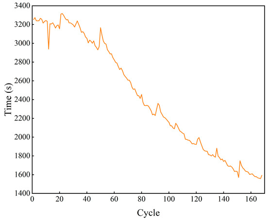
Figure 1.
Constant-current charging time.
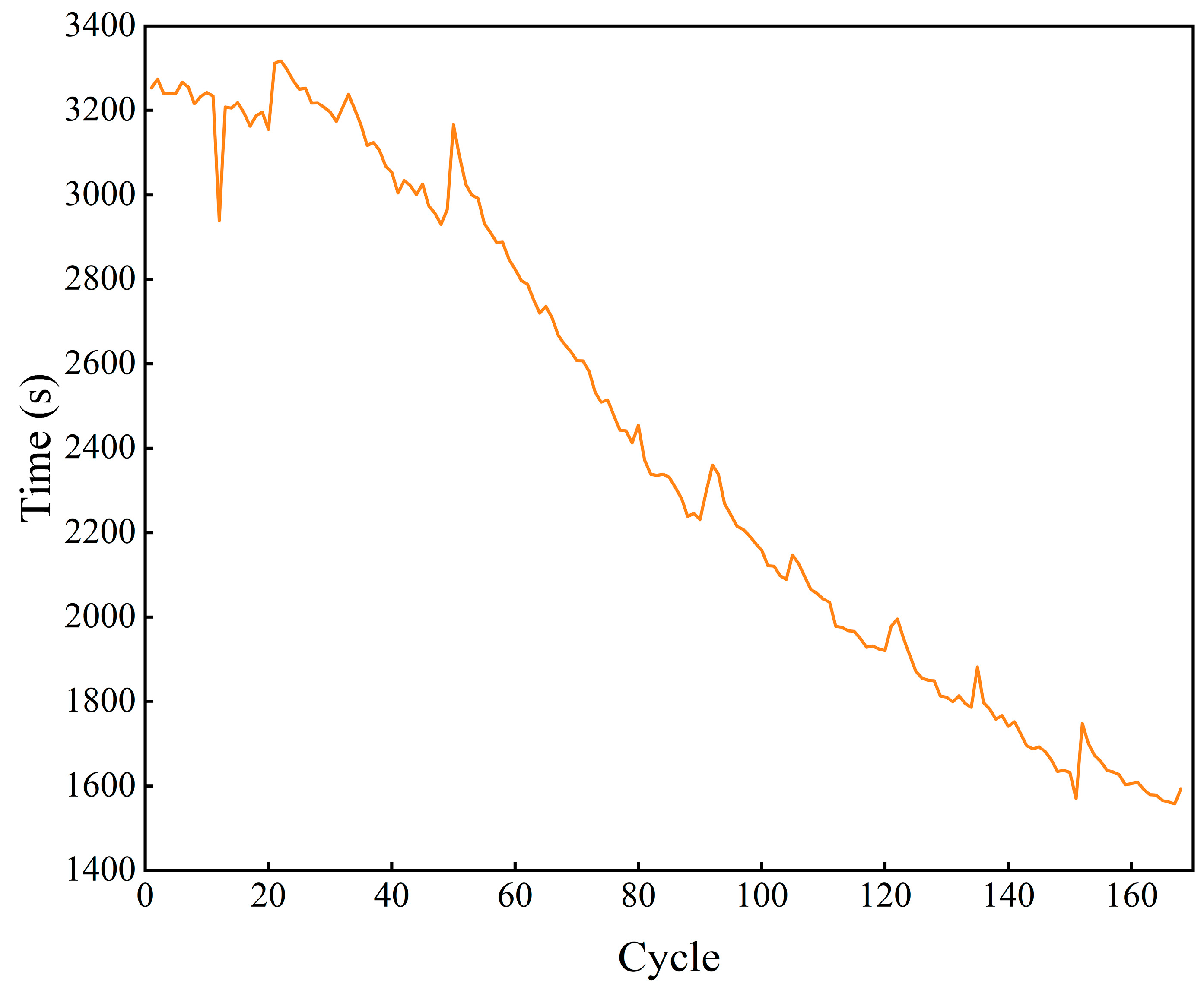
2.2. Constant-Current Discharge Time
In the NASA dataset, the discharging strategy used for the batteries is constant-current discharge, and the constant-current discharge time shows a strong correlation with the battery capacity. Therefore, the constant-current discharge time corresponding to each discharge cycle is extracted, as shown in Figure 2.
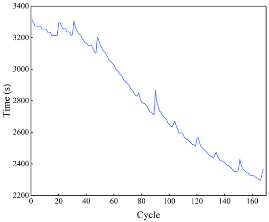
Figure 2.
Constant-current discharge time.
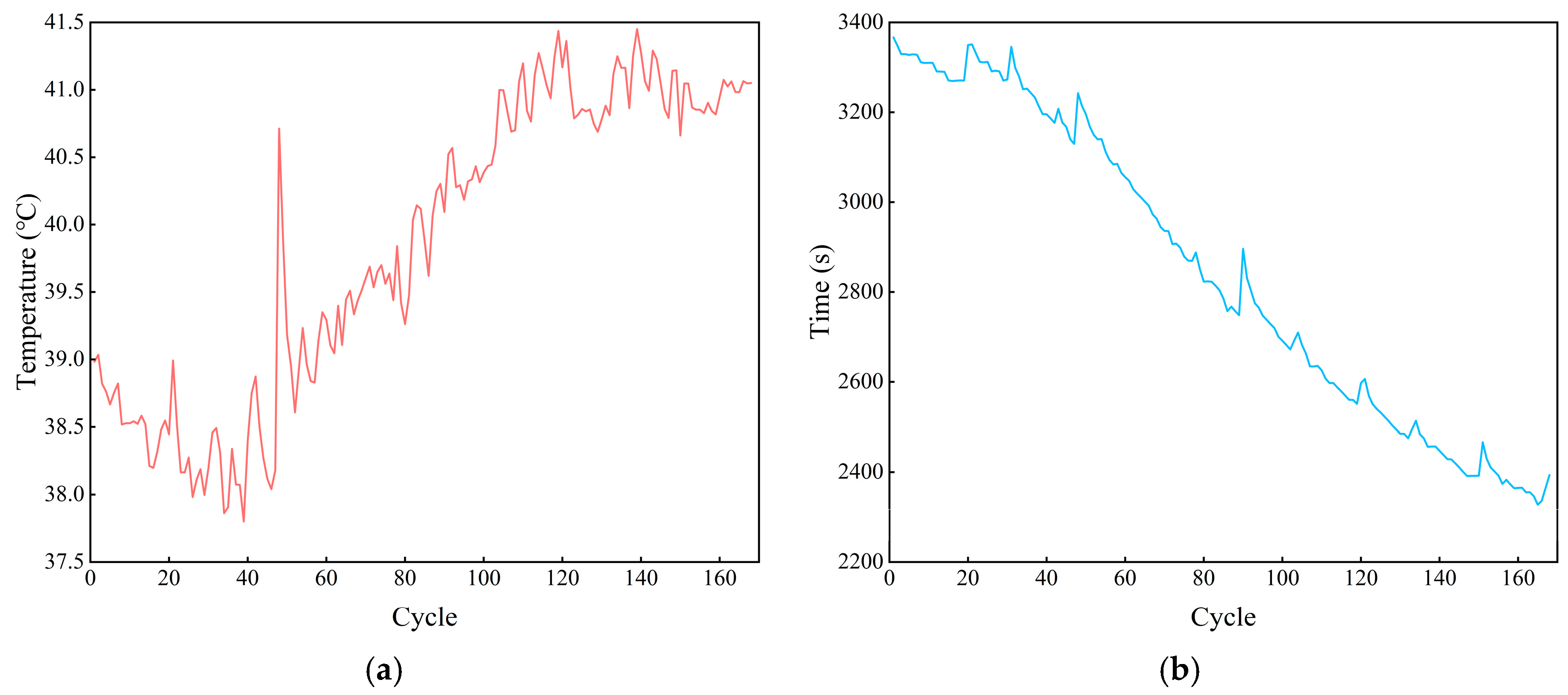
2.3. Maximum Temperature During Discharge Process
Lithium batteries undergo a series of electrochemical reactions during the charging and discharging process, and a large amount of heat is generated at the same time [30]. It is found that, compared with the charging process, the discharging process of lithium batteries generates more heat, and the amount of generated heat in the discharging process gradually increases with an increase in the number of cycles, as shown in Figure 3a. In addition, when the battery is discharged at a certain multiplication rate, the heat is not released in time, making the constant-current discharge time similar to the time at which the temperature reaches its maximum value during the discharge process, as shown in Figure 2 and Figure 3b.
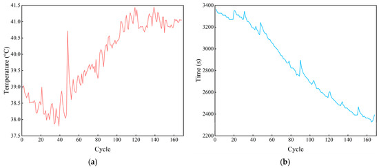
Figure 3.
The temperature-related features during the discharge process: (a) the maximum temperature of the discharge process; (b) the time required for the maximum temperature of the discharge process.
Excessively high temperatures accelerate the rate of electrochemical reaction inside the battery and accelerate the aging of the battery material, as shown in Figure 3b. This accelerated aging of the battery material shortens the time for the discharge process to reach the maximum temperature, and there is a high degree of similarity between the process of change in the time required for the discharge process to reach the maximum temperature and the process of change in the SOH. Therefore, the time required for the discharge process to reach the maximum temperature is taken as the feature to be selected.
2.4. Incremental Capacity Curve of Discharge Process
In the current research on feature extraction for lithium batteries, extracting the incremental capacity (IC) curve contributes to lithium battery characterization and capacity degradation prediction [31,32]. By differentially deriving the voltage and capacity of lithium batteries during the discharge process, the smooth curve is changed to a fluctuating curve, which is more conducive to the analysis of the changing state of the battery capacity [15]. The voltage corresponding to the peak of the IC curve in each cycle is taken as a feature, as shown in Figure 4.
Figure 4.
Voltage characteristics of the discharge process of the B0005 battery.
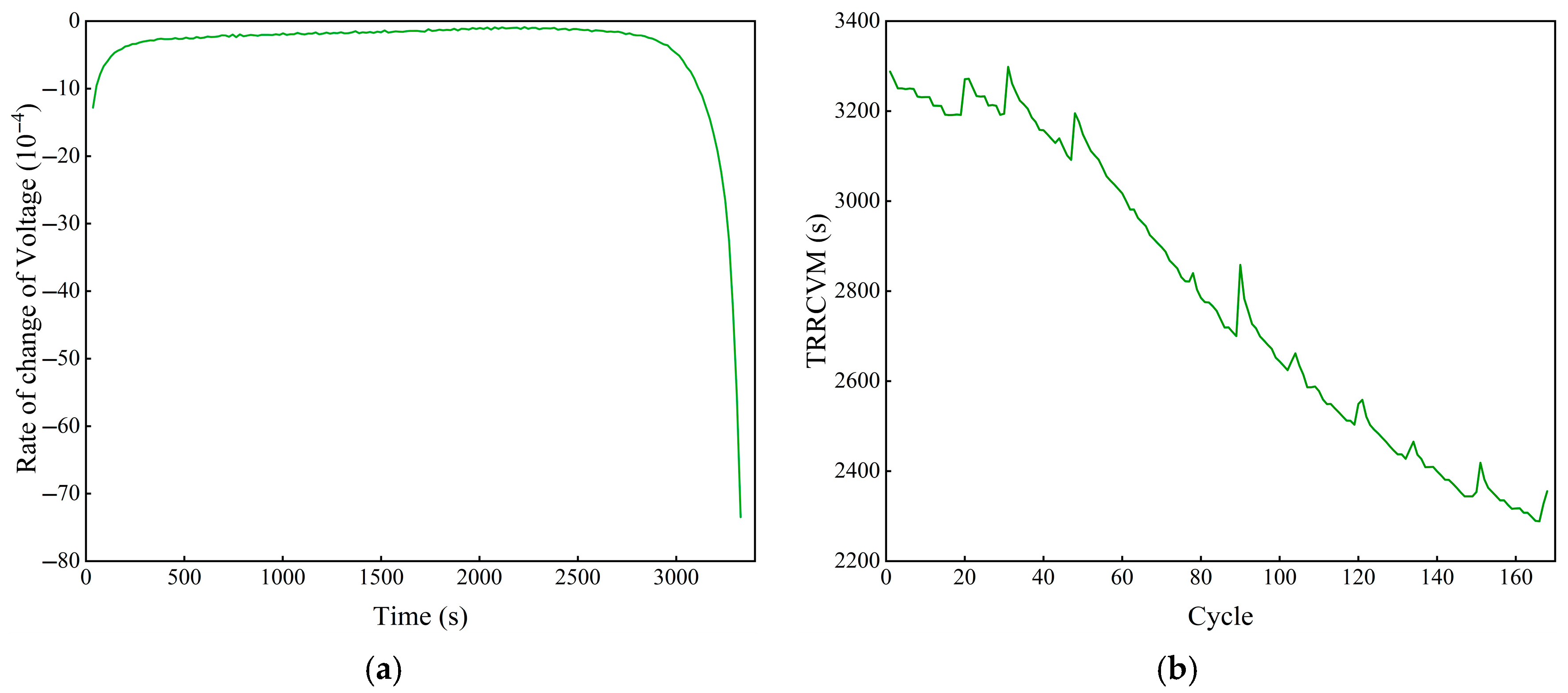
2.5. Rate of Change in Voltage During Discharge Process
In the course of the study, it is found that, as the number of lithium battery cycles increases, the voltage burst of the discharge voltage occurs faster, i.e., the duration of the slow decrease phase of the discharge voltage decreases. The reason for this is that the thickness of the SEI film varies as the discharge process proceeds, which results in a variation in the discharge voltage [33,34]. As shown in Figure 5a, there is a short voltage decrease at the beginning of the discharge process, followed by a long, more stable voltage decrease and finally a voltage plunge phase. As shown in Figure 5b, the time required for the rate of change in the voltage to reach its minimum (TRRCVM) value decreases with the increase in the number of cycles and has a high degree of similarity with the capacity change curve.
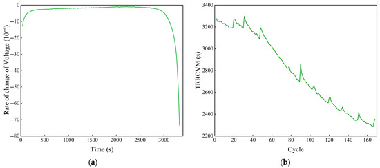
Figure 5.
The rate of change in the voltage feature of the B0005 battery during the discharge process: (a) the rate of change in the voltage of the first discharge cycle; (b) the TRRCVM of all cycles.
3. Lithium Battery SOH Prediction Based on Transfer Learning
3.1. VIW-PSO-VMD Algorithm
In order to achieve the learning of the “capacity resurgence” phenomenon, a signal decomposition framework is proposed. The framework is based on EMD decomposition, combined with PSO to optimize the VMD parameters, and the optimized VMD is applied to the original SOH to extract the high-frequency components and reduce the data volatility. In addition to extracting the high-frequency components, the framework is also able to extract the time-series characteristics of the lithium battery SOH, which assists the model in making accurate predictions. The framework is mainly composed of three parts: improved PSO based on variable inertia weights (VIW), EMD, and VMD.
3.1.1. VIW-PSO
VIW-PSO is an improved algorithm based on the traditional PSO, which is combined with the greedy algorithm [35]. The algorithm evaluates the adaptation of particles through a multivariate evaluation function, while introducing time as an evaluation criterion. The evaluation function is shown in the following equation:
where is the multivariate evaluation function, is the n-th evaluation function, and p is the value produced by PSO.
In the research process, the arrangement entropy, the mean absolute error (MAE) between the original data and the restructured data, and the time are selected as the evaluation functions, which together form . Then, the weights of different particles are calculated based on the multidimensional evaluation value, as shown in the following equation:
where is the weight of the i-th particle.
In the traditional PSO, the inertia weights are set as a decreasing function value from 0.9 to 0.4, which strengthens the search capabilities of the target domain by applying higher inertia weights in the early stage, and stable convergence is achieved by decreasing the inertia weights in the later stage. In order to accelerate the search process in the early stage, VIW is proposed on the basis of PSO, and the calculation formula is as shown below:
where is the variable inertia weight, and t is the number of iterations.
Based on the above formula, the range of values of the variable inertia weights is defined as [0, 1], which not only ensures its significance, i.e., the influence of the current moment on the next moment, but also ensures that the values can present a rapid decline at the beginning of the search, a slow decline in the middle of the search, and stable convergence at the end of the search.
The flow of VIW-PSO is as shown below.
Step 1: Initialize the number, position, and velocity of particles.
Step 2: Calculate the multivariate evaluation index of particles.
Step 3: Determine whether the loop termination condition is reached. If yes, the algorithm is ended; otherwise, the algorithm goes to Step 4.
Step 4: Update the velocity and position of the particles. Specifically, the speed update function is
where is the velocity of the pi-th particle of the i-th iteration; is the single-particle bias coefficient, so that the global optimum is chosen in the range of the single-history optimum. Therefore, the single-particle bias coefficient ensures that the search is directed toward the single-history optimum, and and are the i-th random numbers.
The position update formula is
where is the position of the i-th iteration.
Step 5: Calculate the multivariate evaluation index of the updated particle.
Step 6: Update the historical optimal particle, update the global optimal particle, and go to Step 2.
3.1.2. EMD Process
EMD is a classical signal decomposition algorithm that defines the intrinsic modal components for the first time and uses them as the benchmark for component decomposition. The basic process of the algorithm is as follows: (1) obtain the greatest and smallest values of the data; (2) construct the upper and lower envelopes, as well as the mean envelope; (3) eliminate the mean envelope and check whether the remaining data satisfy the definition of the intrinsic modal component; if they do, the component is eliminated from the original data and (1) to (3) are repeated for the remaining data; if they do not, (1) and (2) are repeated.
EMD allows the noise-laden fluctuation components to be decomposed into a set of smoother, stable components. These components can describe the trends of the original data in the time dimension more clearly; therefore, the components are used as the temporal characteristics of the lithium battery SOH, while the number of components decomposed by EMD is used as the reference value for the K value in the optimization of the VMD parameters of VIW-PSO.
3.1.3. VMD Process
VMD is a decomposition algorithm based on the variational model and achieves the decomposition of the data by continuously solving the variational model. Different from the EMD series of decomposition algorithms, VMD avoids the endpoint effect problem, while the number of components can be customized. Since VMD decomposes the original data through the frequency domain, the extraction of high-frequency components is better facilitated compared to the EMD algorithm, and the capacity for data smoothing is also better than in the EMD decomposition algorithm. During the study, it is found that, after VMD decomposition, the volatility of the components is significantly lower than that after EMD decomposition, and the volatility and standard deviations (SDs) of the components are compared in Table 1, taking B0005 as an example.

Table 1.
A comparison of different signal decomposition algorithms.
While the number of customized components in VMD improves the range of its application, it also limits its decomposition performance. It is prone to under-decomposition when the value of K is low, so that high-frequency noise still exists in the components, and over-decomposition when the value of K is high. Therefore, the EMD decomposition results are used as a benchmark, and the parameters of VMD are optimized by combining it with VIW-PSO.
3.2. T-Pearson Correlation Analysis Algorithm
This paper proposes the T-Pearson correlation analysis algorithm, combining trend correlation coefficients and Pearson correlation coefficients as a means of avoiding the limitations associated with assessing only the linear correlations between the features and lithium battery SOH.
The trend correlation analysis algorithm is a method proposed by the authors of this paper to measure the correlation of the data in a time series, which is mainly reflected in measuring the trends of the data. Different from the commonly used correlation analysis algorithms, trend correlation analysis evaluates the similarity of different sequences of data in a time series by comparing whether there is consistency in the changes between the current moment and the next moment. The specific calculation steps are shown below.
Step 1: Calculate the change in sequence and sequence at the current moment and the next moment:
where is the original length of the data, is the length of the sequence of changes, and ; is the change in the data at moment of sequence .
Step 2: Return a value of 1 if the changes are the same or 0 otherwise:
where is the trend correlation index at the t-th time.
Step 3: Calculate the overall trend correlation:
where is the trend correlation index of sequence A and sequence B.
The similarity of two sets of data in terms of change trends can be measured by comparing the change values of the two sets of data at the current moment with those at the previous moment. However, there is a limitation in selecting features only via the similarity in the change trend, i.e., the similarity of the data in the linear change cannot be measured. Therefore, by combining Pearson correlation analysis and trend correlation analysis, the T-Pearson correlation analysis algorithm is proposed, as shown in the following equation:
where is the Pearson correlation index between A and B.
The combined correlations are expressed as means by calculating trend correlations and Pearson correlation coefficients between the features and SOH.
3.3. Linear Regression Convolutional Neural Network Model
Existing lithium battery SOH prediction models need to be retrained to learn new parameters after accessing new data, especially when the trained model is applied on other datasets, and the prediction performance of the model will be affected to a high degree. To learn dataset-specific features as well as common features across different datasets, enabling the model to achieve high-precision predictions on new datasets with the same structure and weights, based on high-precision predictions on the training dataset, the linear regression convolutional neural network (LRCNN) model is proposed. The model consists of four parts.
- (1)
- Trend feature learning model. This module is based on LR, seeking to learn the mapping relationship between historical data and the current data in a specific dataset, thereby extracting the development trend of the specific dataset as a feature. Lithium battery SOH data differ from other time-series data in that they have weaker volatility and a more pronounced downward trend within a cycle, with the linear characteristics being particularly evident. After decomposing the raw data using VMD, the data with the core trend can be obtained, enabling LR to learn the core trend in the data.
- (2)
- Feature concatenation module. This module concatenates trend features and strongly correlated physical features selected by T-Pearson through a concatenation layer.
- (3)
- Common feature learning module. The correlation between the lithium-ion battery SOH data and physical features from different data sources exhibits a certain degree of similarity. Therefore, a convolutional neural network is used to learn the mapping between strongly correlated physical features and SOH data. To accommodate the uniqueness of data from different sources, the trend features of the data are concatenated and fused with the strongly correlated physical features to achieve the learning of common features.
- (4)
- Prediction module. Finally, the lithium battery SOH data are predicted through a fully connected layer.
3.3.1. Trend Feature Extraction Block
LR is a classic machine learning algorithm, and its ordinary form can be expressed as shown in Equation (13):
where are the input features; are the linear weights corresponding to different inputs, respectively; and is the intercept.
Through Equation (13), it can be seen that the LR model is able to achieve better prediction performance in the face of a small-sample dataset, and the trained model has strong interpretability, being able to represent the effects of different features on the data to be predicted. However, although LR has more stable and better prediction performance than neural networks under small-sample datasets, it requires a linear relationship between the input data and output data, and it is difficult for LR to achieve better prediction performance for nonlinear prediction tasks. Therefore, the linear relationship among lithium battery SOH data is analyzed.
Firstly, the historical data are reconstructed in terms of the time window by reconstructing the original data into . The size of the time window is , and the structure of the reconstructed data is as shown in the following equation:
where is the original dataset, is the length of the original dataset, and is the window size.
Then, the Pearson correlation coefficient between the corresponding value in each window and the current SOH is calculated, as shown in Equation (15) to Equation (17). In the case of type B0005, for example, is set to 3, i.e., the original data are reconstructed with a time window of size 3. Since EMD decomposition is performed prior to this, the original data at this time are component data, and the Pearson correlation coefficients between the corresponding values of the time window composing the data and the data to be predicted are as shown in Table 2.
Table 2.
Correlations between different corresponding values in the time window and the data to be predicted.
Table 2 shows that there is a strong correlation between the historical data and the data to be predicted, so LR can be used as a training model for trend features to learn the linear mapping relationships between the historical data and the data to be predicted, and the trend features can be extracted for the specific data.
A neural network is an effective tool to achieve SOH prediction, and it can learn the nonlinear features between the SOH data and physical features. However, due to the small size of the dataset, the neural network cannot correct features precisely; as a result, the model’s performance is very unstable. In contrast, LR can achieve accurate prediction with a small-sized dataset. In order to confirm that LR has higher performance than a neural network when the dataset is small, LR and several neural networks are compared via the MAE, root mean square error (RMSE), and coefficient of determination (R2), and the results are shown in Table 3. The neural networks include BP, long short-term memory (LSTM), and CNN-LSTM.
Table 3.
The comparison of LR and neural networks.
As can be seen from Table 3, the neural networks’ performance is worse than that of LR in trend feature prediction, especially regarding the R2, where the scores of LSTM and CNN-LSTM are less than 0. The core reason is the features of the trend curve. The trend curve provided by VMD is a smooth curve, and the length of the curve is short, which means that the neural network cannot learn the correct features.
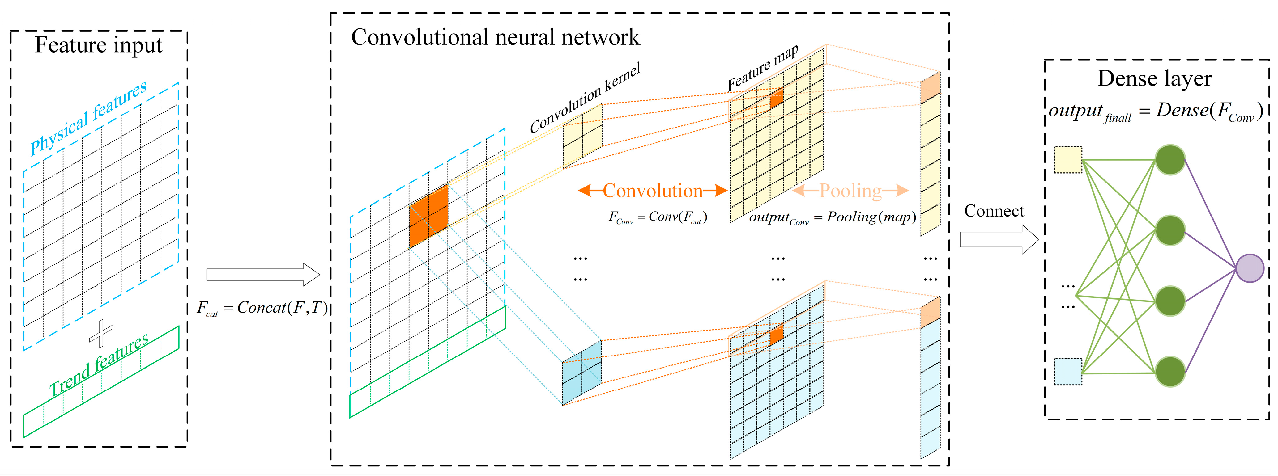
3.3.2. Feature Fusion Model
A model that only learns the trend features is unable to achieve accurate prediction on different datasets, so it also needs to learn the common features. According to the electrochemical mechanism of battery charging and discharging, as well as the discussion in Section 2.2, it can be seen that the SOH of lithium batteries is related to their physical features. Therefore, common features of different categories of batteries can be extracted based on the physical features of lithium batteries. Meanwhile, in order to strengthen the learning ability of the model regarding the features of different datasets, the trend features are combined with the strongly correlated physical features and then fused and extracted by a CNN, as shown in the following equation:
where is the spliced features, is the strongly correlated physical features, and is the trend features obtained based on LR.
A convolution operation is then performed on the spliced features using the convolution layer, as shown in Equation (19):
where is the value of the output sequence at position i and channel d, i.e., the convolutional output value of the i-th spliced feature at the d-th convolutional kernel; is the weight of the d-th convolutional kernel at the m-th position, where the input channel is ; and is the bias term of the output channel d.
After the convolution operation, the trend features are fused with the strongly correlated physical features, and their common features are learnt; these are then input into the subsequent fully connected layer for feedforward training to finally obtain the predicted values of the components. The flow of the LRCNN is shown in Figure 6.
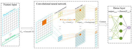
Figure 6.
LRCNN flow chart.
3.4. Transfer Learning Based on Time Feature Analysis
After learning trend features and common features via the LRCNN, the model is initially equipped with cross-dataset feature learning capabilities, and, after training on a single dataset, it can achieve higher-accuracy prediction on other datasets. However, in order to further improve the prediction performance of the trained model on other datasets and increase the efficiency of the model, migration learning based on temporal feature analysis is proposed. After calculating the sample entropy and alignment entropy of the source-domain dataset and the target-domain dataset, the multiple entropy values are used to measure their temporal features, and migration learning is performed by selecting source and target domains with similar temporal features. The steps are shown in Figure 7. Meanwhile, in order to improve the accuracy and training efficiency, the following operations are carried out in the process of migration learning:
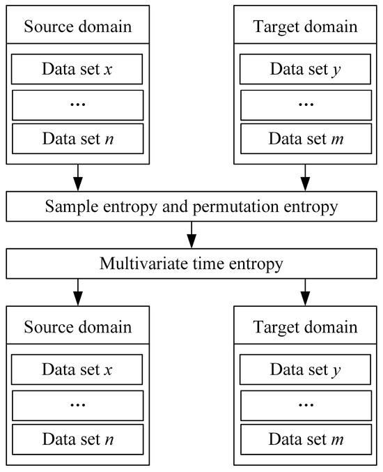
Figure 7.
Transfer learning based on temporal feature analysis.
- (1)
- Freeze all but the last layer and train only the output weights of the last layer;
- (2)
- Use a smaller learning rate and number of epochs.
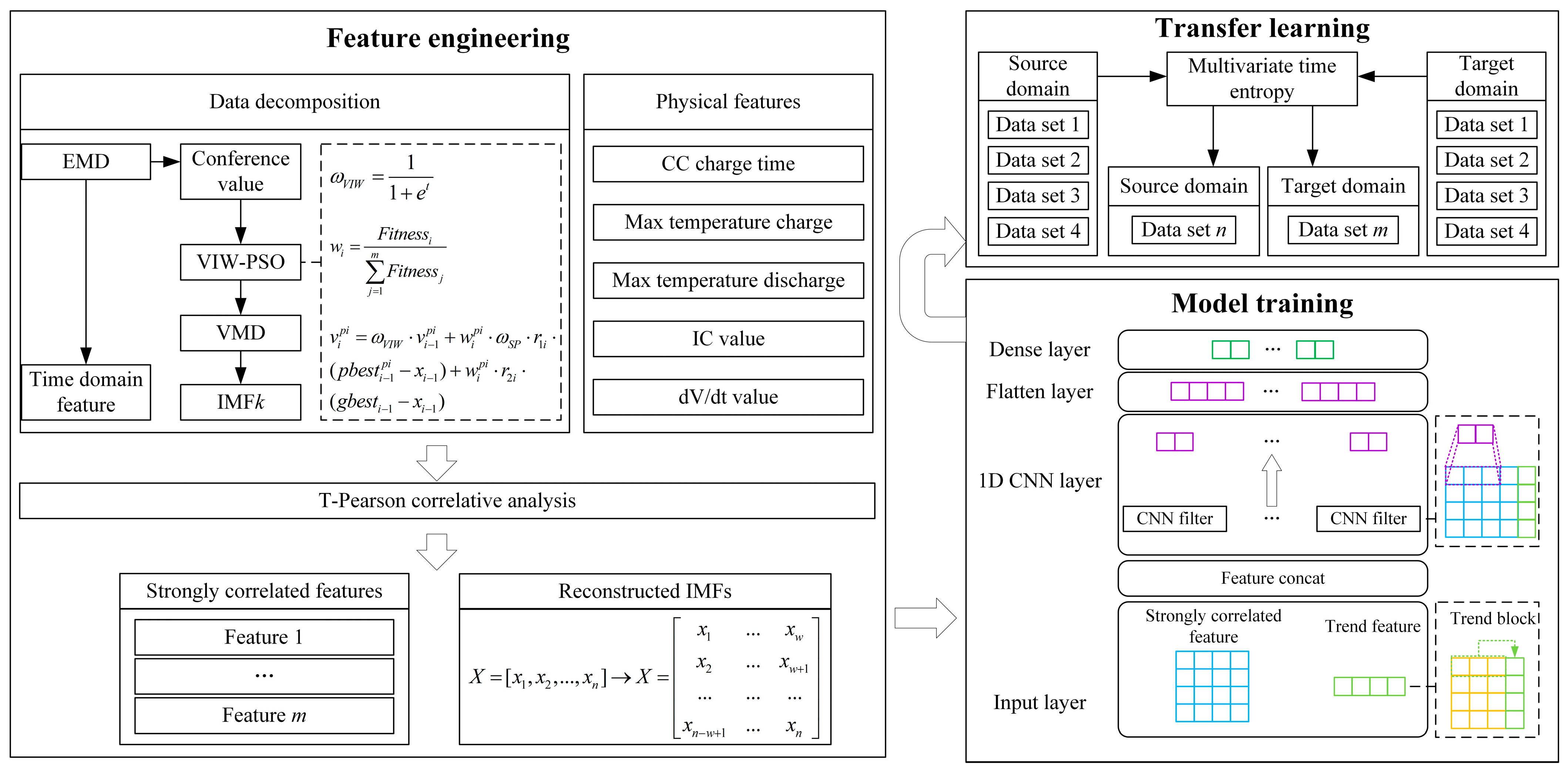
3.5. Proposed Prediction Framework
The proposed framework for lithium battery SOH prediction is shown in Figure 8.
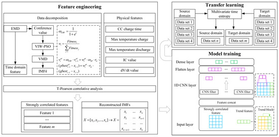
Figure 8.
Proposed SOH prediction framework for lithium batteries.
4. Results and Analysis
4.1. Dataset
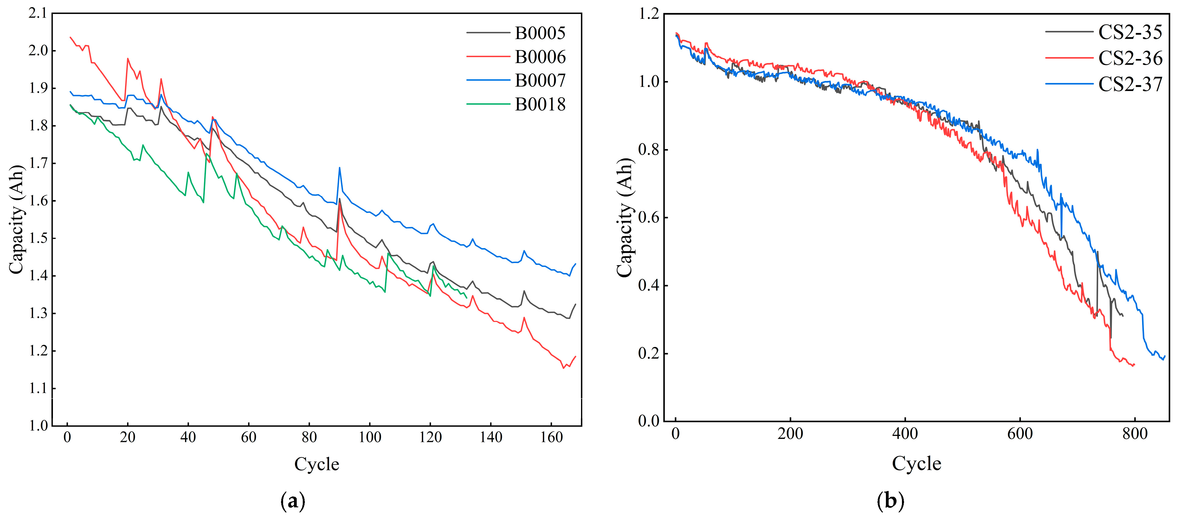
The datasets used in this paper include the lithium battery datasets from the NASA Ames Research Center and the Center for Advanced Life Cycle Engineering (CALCE) team at the University of Maryland. Among these, B0005, B0006, B0007, B0018, and CS2-35, and CS2-37 are selected as the data, and their capacity variations are shown in Figure 9. The B0005, B0006, B0007, and B0018 batteries are the same types of batteries, with a capacity of 2 Ah and a constant-current and constant-voltage (CC-CV) charging and discharging strategy. The CS2-35 and CS2-37 batteries are the same types of batteries, with a capacity of 1100 mAh and a CC-CV charging and discharging strategy.

Figure 9.
Battery capacity change curves: (a) NASA dataset; (b) CALCE dataset.
4.2. Case Study Conditions and Dataset Division
In order to validate the performance of the proposed lithium battery SOH estimation method, method validation and model comparison experiments are carried out on a desktop computer equipped with an Inter Core i5-10400 CPU and Inter UHD Graphics 630. The software platform is PyCharm Community Edition 2023.1.
The B0005, B0006, and B0007 batteries have 168 cycles; the B0018 battery has 132 cycles; and the CS2-35 and CS2-37 batteries have 779 and 852 cycles, respectively. In order to prove that the proposed method has better prediction performance compared with the existing methods, random scaling is used to separate the test set and prediction set, and the datasets are divided separately based on the division methods demonstrated in different existing studies.
4.3. Evaluation Accuracy Indicators
In order to evaluate the prediction performance of the proposed method, the MAE, RMSE, and R2 are chosen as the evaluation metrics, with the formulas shown in the following equations:
where n is the number of test data, is the i-th prediction value, is the i-th true value, and is the average value of the true values.
4.4. Comparison and Analysis of Different Decomposition Algorithms
In order to verify that the proposed VIW-PSO-VMD has better decomposition performance, ablation experiments are conducted to compare it with PSO-VMD. The ablation function is a multivariate ablation function combining the permutation entropy, the MAE of the original and reconstructed data, and the time. We apply the optimality-seeking stopping condition, the overall number of iterations is set to 50, and stopping is implemented after 50 iterations. Table 4 shows the comparison results for VIW-PSO and PSO.
Table 4.
The comparison of VIW-PSO and PSO.
From Table 4, it can be seen that VIW enables PSO to perform more efficient parameter seeking, and its seeking results have better adaptation scores compared to those of ordinary PSO.
Next, the prediction performance of the models under different decomposition algorithms is compared. The main decomposition algorithms used are EMD, complete ensemble empirical mode decomposition (CEEMD), VMD-EMD, and VMD. The comparison results are shown in Table 5.
Table 5.
The impacts of different decomposition algorithms on the predictive model.
From Table 5, it can be seen that EMD and CEEMD are unable to achieve accurate decomposition, causing the features of other components to exist between different components and thus reducing the prediction accuracy. Meanwhile, the quadratic VMD-EMD method is able to achieve better prediction accuracy but at the cost of becoming longer. VMD sets the K value as the reference value from EMD, but it still has significant modal aliasing. After optimization, VMD obtains the best value from VIW-PSO, and it achieves the best decomposition performance.
4.5. Correlation Analysis and Strongly Correlated Feature Extraction
The SOH of lithium batteries is closely related to their states during charging and discharging. In order to extract multiple covariates that are the most relevant to the SOH trends of lithium batteries, and to reduce the influence of weakly correlated covariates on the model performance, the correlations are measured using the T-Pearson correlation analysis method. Taking the B0005 battery as an example, its specific correlations are as shown in Table 6.
Table 6.
The correlations between different physical features and the SOH of a lithium battery.
In terms of linear correlations, the correlations between all of the selected features and the SOH of lithium batteries are high, and their absolute values are all greater than 0.8; however, in terms of trend correlations, the correlation between the constant-current discharge time, the time required for the discharge process to reach the maximum temperature, and the time required for the rate of change in the voltage to reach the minimum in the discharge process and the SOH of the lithium battery is higher. Meanwhile, the maximum temperature of the discharge process is negatively correlated with the SOH, and the trend correlation is positively stemmed, resulting in a weaker T-Pearson correlation. The linear correlation is negative, while the trend correlation is positive, which leads to a weak T-Pearson correlation.
Therefore, according to the results of the T-Pearson analysis of all features, the constant-current discharge time, the time required to reach the maximum temperature in the discharge process, and the time required for the rate of change in the voltage in the discharge process to reach the minimum value are taken as the strongly correlated physical features.
In order to demonstrate the advantage of T-Pearson in feature selection, the performance of Pearson-selected features and T-Pearson-selected features on the prediction model is compared. The results are shown in Table 7.
Table 7.
The comparative results between different correlation analysis methods.
As can be seen from Table 7, T-Pearson is able to select more accurate and strongly correlated features to improve the predictive performance of the model.
The lithium battery SOH yields time-series data, and the temporal features are equally important for lithium battery SOH prediction, so the time-series features of the lithium battery SOH are extracted by EMD. Then, the correlations between the time-series features and the SOH of lithium batteries are analyzed using T-Pearson correlation analysis; the results are shown in Table 8.
Table 8.
The correlations between different components and the SOH of a lithium battery.
Table 8 shows that, although the linear correlation between IMF4 and SOH is high, the T-Pearson correlation does not reach the threshold due to its low trend correlation.
4.6. Predictive Performance of Proposed Model on Other Datasets
In order to achieve the same high prediction performance of the model on other datasets, the proposed SOH prediction framework improves the generalization of the model via two methods: (1) combining the trend features of a single dataset with the strongly correlated features and learning the common features through a CNN; (2) using migration learning based on temporal feature analysis and achieving the cross-domain training of the model by freezing the network and fine-tuning the parameters. The results of the multivariate temporal entropy calculations for different types of batteries in the NASA dataset and CALCE dataset are shown in Table 9.
Table 9.
Multivariate time entropy for different datasets.
Table 9 shows that the multivariate temporal entropy of the B0005 dataset is the closest to that of B0018 in the NASA dataset, and the multivariate temporal entropy of CS2-35 is the closest to that of CS2-37 in the CALCE dataset. Therefore, under the premise of using B0005 as the source-domain dataset, since B0018 is the closest to it in terms of time-domain features, B0018 is used as the target domain to achieve the cross-domain training of the model by freezing the network layers, as well as fine-tuning the parameters, and the model is able to achieve higher prediction performance. Taking B0005 and B0018 as examples, the specific parameters of migration learning are as shown in Table 10. During the training phase of the source domain, the structure of the model is as shown in Table 10, and the total parameter count is 4183. The number of epochs is 200, and the training time is 22 s.
Table 10.
Transfer learning operational parameters.
By freezing the convolutional layer and preserving the degree of learning for common features, the fully connected layer achieves higher prediction accuracy with a lower learning rate and epoch number according to different datasets. Taking B0005 and CS2-35 as the source domains, the model’s performance after migration learning, as well as the model’s performance before migration learning, is shown in Table 11.
Table 11.
Comparison of prediction performance before and after migration learning.
As can be seen from Table 11, after temporal feature selection, the model still has better prediction performance even without migration when the temporal characteristics of the target and source domains are similar, and the prediction performance of the model is further improved after migration learning. Compared with other datasets, B0006 has a minimal performance gap before and after transfer learning, and the reason is that it is similar to B0005 in term of multivariate time entropy, and the model can achieve good performance without transfer learning. After training, the model can accurately map the input data of the B0006 dataset to the predicted data of the B0006 dataset. Although the B0006 dataset yields a smaller improvement in the prediction performance of the model before and after migration learning, in terms of training efficiency, migration learning can achieve more efficient prediction performance with a lower learning rate and fewer epochs.
4.7. Predictive Performance of Proposed Model on Small-Sample Dataset
The LRCNN can learn the trend features and common features via a trend feature learning model and common feature learning model, and the common feature learning model is the most important part. The structure of the common feature learning model affects the prediction performance. Thus, the different structures are compared, and the results are shown in Table 12.
Table 12.
A comparison of the different structures.
As can be seen from Table 12, the model that has two CNN layers has the worst performance. The reason is that the features obtained by two CNN layers cannot accurately map the data to be predicted. The excessive number of layers leads to overfitting. Thus, one CNN is the best structure.
Small samples are one of the problems faced during lithium battery SOH prediction. The proposed SOH prediction framework achieves the accurate estimation of trends under small-sample datasets through an internal trend block, which in turn improves the prediction ability of the whole prediction framework on small-sample datasets. Taking B0005 as an example, 20 cycles, 40 cycles, and 60 cycles are used as the training set, and its solutions are shown in Table 13.
Table 13.
Predictive performance of the proposed method on small-sample datasets of different sizes.
As can be seen from Table 13, the proposed prediction framework can still achieve high prediction accuracy on small-sample datasets. Meanwhile, due to the strong linear relationship among SOH data on a single type of battery, and the fact that the CNN is a nonlinear neural network, its performance on linear datasets will have an impact on the overall prediction performance. Thus, the table shows that there is a slight decrease in the performance of the model with an increase of the size of the training set. Regarding the LR model, although, on a single type of battery SOH data, it can accurately capture trends, its trained model is difficult to apply to other types of batteries. Therefore, CNNs are needed to learn the common features so as to improve the generalization ability of the model.
4.8. Comparison with Other Methods
In order to objectively evaluate the performance of the proposed method in lithium battery SOH prediction and highlight its advantages in terms of prediction performance, it is compared with several mainstream methods, and the comparison results are shown in Table 14 and Table 15. M1–M8 are specified as follows.
Table 14.
The results of the comparison with popular prediction methods.
Table 15.
The results of the comparison with CALCE.
M1: The model uses LSTM to predict the SOH of Li-ion batteries and improves the sparrow optimization algorithm (SSA) to optimize the parameters of LSTM to improve the prediction accuracy.
M2: The model convolves the features obtained by the CNN to extract the features with strong representation capabilities; it then learns the temporal features via LSTM and finally predicts them via a deep feedforward network (DNN).
M3: The model uses multi-population evolution whale optimization algorithm-optimized variational mode decomposition to optimize the parameters of VMD and decompose the SOH, followed by component prediction via a Transformer.
M4: The model uses a Gaussian regression model to predict the SOH.
M5: The model performs prediction using support vector regression (SVR) after decomposing the data via ensemble empirical mode decomposition (EEMD), while the parameters of SVR are optimized using the grey wolf optimizer (GWO).
M6: The model combines CNN-LSTM with an attention mechanism and uses Pearson correlation analysis and Spearman correlation analysis to extract strongly correlated features.
M7: The model decomposes the data via complete ensemble empirical mode decomposition with adaptive noise (CEEMDAN) and then predicts the components via CNN-LSTM.
M8: The model selects the features through grey relation analysis and predicts the SOH data via Gaussian process regression.
From Table 14 and Table 15, it can be seen that the proposed method has a more obvious improvement in the prediction accuracy. VIW-PSO-VMD helps the model to extract the high-frequency components in the original data and transform them into smoother components. The strongly correlated features extracted with T-Pearson aid the model’s learning and reduce the impact of weakly correlated features on the model’s prediction performance. The LRCNN extracts and fuses the trend features and common features, which improves the generalization ability of the model. Transfer learning based on time-domain feature analysis helps the model to achieve cross-domain learning and, at the same time, improves the training efficiency of the model. Although there are some models that outperform the proposed framework, migration learning is able to achieve higher training efficiency.
5. Conclusions
The accurate prediction of the lithium battery SOH is crucial for charging and discharging efficiency, as well as the charging and discharging capacity of an energy storage power plant. In this paper, we propose a novel SOH prediction method for lithium-ion batteries. The main contributions of our framework include (1) demonstrating that the time required to reach the minimum value of the voltage change rate during discharge can accurately reflect lithium battery health degradation trends, thereby enhancing feature space representation for SOH prediction; (2) the development of T-Pearson, a comprehensive correlation analysis method that evaluates multivariate feature–SOH relationships from multiple dimensions to precisely extract strongly correlated features; (3) the proposed LRCNN model’s ability to effectively learn both the trend characteristics of the battery SOH and the nonlinear degradation patterns when combined with strongly correlated features, enabling high-precision predictions across diverse datasets; (4) the introduction of temporal feature analysis-based transfer learning, which significantly improves the model’s cross-domain learning ability and enables adaptive high-precision predictions using a single model architecture, thereby enhancing the generalizability.
Future work will include exploring features with stronger hidden information representation capabilities and feature splicing methods with the dynamic adjustment of different feature weights.
Author Contributions
Conceptualization, Y.X. and H.L.; methodology, Z.Z.; software, T.L. and Z.Z.; validation, L.G. and Z.Z.; formal analysis, H.L.; investigation, Y.X.; resources, T.L.; data curation, Y.X.; writing—original draft preparation, Y.X.; writing—review and editing, Y.X. and T.L.; visualization, L.G.; supervision, J.H.; project administration, T.L. and H.L. All authors have read and agreed to the published version of the manuscript.
Funding
This research was funded by China Yangtze Power Co., Ltd., grant number Z412302065.
Data Availability Statement
The data presented in this study are available at [https://www.nasa.gov/intelligent-systems-division/discovery-and-systems-health/pcoe/pcoe-data-set-repository/, accessed on 1 May 2025].
Conflicts of Interest
Authors Yuchao Xiong and Tiangang Lv were employed by Three Gorges Electric Energy Co., Ltd. Author Liya Gao was employed by Hubei Qingjiang Hydropower Development Co., Ltd. The remaining authors declare that the research was conducted in the absence of any commercial or financial relationships that could be construed as a potential conflict of interest.
Abbreviations
The following abbreviations are used in this manuscript:
| BP | Backpropagation |
| CNN | Convolutional neural network |
| CEEMD | Complete ensemble empirical mode decomposition |
| CEEMDAN | Complete ensemble empirical mode decomposition with adaptive noise |
| DNN | Deep feedforward network |
| EMD | Empirical mode decomposition |
| EEMD | Ensemble empirical mode decomposition |
| GWO | Grey wolf optimizer |
| IC | Incremental capacity |
| LSTM | Long short-term memory |
| MAE | Mean absolute error |
| PSO | Particle swarm optimization |
| RMSE | Root mean square error |
| R2 | Coefficient of determination |
| SC | Start cycle |
| SOH | State of health |
| SEI | Solid electrolyte interphase |
| SVR | Support vector regression |
| TCMPSO | Tripartite competition mechanism PSO |
| TRRCVM | Time required for rate of change in voltage to reach its minimum |
| VIW | Variable inertia weight |
| VMD | Variational mode decomposition |
References
- Farivar, G.G.; Manalastas, W.; Tafti, H.D.; Ceballos, S.; Sanchez-Ruiz, A.; Lovell, E.C.; Konstantinou, G.; Townsend, C.D.; Srinivasan, M.; Pou, J. Grid-Connected Energy Storage Systems: State-of-the-Art and Emerging Technologies. Proc. IEEE 2022, 111, 397–420. [Google Scholar] [CrossRef]
- Chen, S.; Sun, C.; Zhang, H.; Yu, H.; Wang, W. Electrochemical Deposition of Bismuth on Graphite Felt Electrodes: Influence on Negative Half-Cell Reactions in Vanadium Redox Flow Batteries. Appl. Sci. 2024, 14, 3316. [Google Scholar] [CrossRef]
- Mlilo, N.; Brown, J.; Ahfock, T. Impact of intermittent renewable energy generation penetration on the power system networks—A review. Technol. Econ. Smart Grids Sustain. Energy 2021, 6, 1–19. [Google Scholar] [CrossRef]
- Zheng, R.; Yang, B.; Qian, Y.; Li, H.; Gao, D.; Jiang, L. Joint SOH and RUL estimation for lithium-ion batteries via optimal deep belief network with Bayesian algorithm. J. Energy Storage 2025, 131, 115891. [Google Scholar] [CrossRef]
- Fang, X.; Chen, Z.; Li, J. Optimized multi-head self-attention mechanism for SOH prediction in lithium-ion battery energy storage systems within microgrids. Electr. Power Syst. Res. 2024, 238, 111182. [Google Scholar] [CrossRef]
- Lin, C.; Xu, J.; Shi, M.; Mei, X. Constant current charging time based fast state-of-health estimation for lithium-ion batteries. Energy 2022, 247, 123556. [Google Scholar] [CrossRef]
- Li, C.; Yang, L.; Li, Q.; Zhang, Q.; Zhou, Z.; Meng, Y.; Zhao, X.; Wang, L.; Zhang, S.; Li, Y.; et al. SOH estimation method for lithium-ion batteries based on an improved equivalent circuit model via electrochemical impedance spectroscopy. J. Energy Storage 2024, 86, 111167. [Google Scholar] [CrossRef]
- Xu, Z.; Wang, J.; Lund, P.D.; Zhang, Y. Co-estimating the state of charge and health of lithium batteries through combining a minimalist electrochemical model and an equivalent circuit model. Energy 2022, 240, 122815. [Google Scholar] [CrossRef]
- Guo, F.; Wu, X.; Liu, L.; Ye, J.; Wang, T.; Fu, L.; Wu, Y. Prediction of remaining useful life and state of health of lithium batteries based on time series feature and Savitzky-Golay filter combined with gated recurrent unit neural network. Energy 2023, 270, 126880. [Google Scholar] [CrossRef]
- Pan, R.; Liu, T.; Huang, W.; Wang, Y.; Yang, D.; Chen, J. State of health estimation for lithium-ion batteries based on two-stage features extraction and gradient boosting decision tree. Energy 2023, 285, 129460. [Google Scholar] [CrossRef]
- Zhou, Y.; Dong, G.; Tan, Q.; Han, X.; Chen, C.; Wei, J. State of health estimation for lithium-ion batteries using geometric impedance spectrum features and recurrent Gaussian process regression. Energy 2022, 262, 125514. [Google Scholar] [CrossRef]
- Wen, J.; Chen, X.; Li, X.; Li, Y. SOH prediction of lithium battery based on IC curve feature and BP neural network. Energy 2022, 261, 125234. [Google Scholar] [CrossRef]
- Xia, F.; Yu, Y.; Chen, J. SOH and RUL prediction of lithium batteries based on fusions of RLOESS filtered electrochemical and thermal features by bidirectional gated recurrent unit network. J. Energy Storage 2024, 102, 114134. [Google Scholar] [CrossRef]
- Zhou, D.; Liang, J.; Li, F.; Cui, Y.; Shan, Y.; Zhang, Y.; Chen, M.; Li, S. SOH prediction of lithium-ion batteries using a hybrid model approach integrating single particle model and neural networks. J. Energy Storage 2024, 104, 114579. [Google Scholar] [CrossRef]
- Dai, H.; Wang, J.; Huang, Y.; Lai, Y.; Zhu, L. Lightweight state-of-health estimation of lithium-ion batteries based on statistical feature optimization. Renew. Energy 2023, 222, 119907. [Google Scholar] [CrossRef]
- Sun, J.; Fan, C.; Yan, H. SOH estimation of lithium-ion batteries based on multi-feature deep fusion and XGBoost. Energy 2024, 306, 119907. [Google Scholar] [CrossRef]
- Lin, M.; Ke, L.; Wang, W.; Meng, J.; Guan, Y.; Wu, J. Health prognosis via feature optimization and convolutional neural network for lithium-ion batteries. Eng. Appl. Artif. Intell. 2024, 133, 108666. [Google Scholar] [CrossRef]
- Zhu, T.; Wang, S.; Fan, Y.; Hai, N.; Huang, Q.; Fernandez, C. An improved dung beetle optimizer- hybrid kernel least square support vector regression algorithm for state of health estimation of lithium-ion batteries based on variational model decomposition. Energy 2024, 306, 132464. [Google Scholar] [CrossRef]
- Fu, J.; Wu, C.; Wang, J.; Haque, M.; Geng, L.; Meng, J. Lithium-ion battery SOH prediction based on VMD-PE and improved DBO optimized temporal convolutional network model. J. Energy Storage 2024, 87, 111392. [Google Scholar] [CrossRef]
- Yuan, Z.; Tian, T.; Hao, F.; Li, G.; Tang, R.; Liu, X. A hybrid neural network based on variational mode decomposition denoising for predicting state-of-health of lithium-ion batteries. J. Power Sources 2024, 609, 234697. [Google Scholar] [CrossRef]
- Cheng, G.; Wang, X.; He, Y. Remaining useful life and state of health prediction for lithium batteries based on empirical mode decomposition and a long and short memory neural network. Energy 2021, 232, 121022. [Google Scholar] [CrossRef]
- Ma, Z.; Han, J.; Chen, H.; Houari, A.; Saim, A. Research on power allocation strategy and capacity configuration of hybrid energy storage system based on double-layer variational modal decomposition and energy entropy. J. Energy Storage 2024, 95, 112492. [Google Scholar] [CrossRef]
- Huang, K.; Yao, K.; Guo, Y.; Lv, Z. State of health estimation of lithium-ion batteries based on fine-tuning or rebuilding transfer learning strategies combined with new features mining. Energy 2023, 282, 128739. [Google Scholar] [CrossRef]
- Liu, Y.; Liu, Y.; Shen, H.; Ding, L. Battery state of health estimation using a novel BiLSTM-Mamba2 network with differential voltage features and transfer learning. J. Energy Storage 2025, 110, 115347. [Google Scholar] [CrossRef]
- Fu, S.; Tao, S.; Fan, H.; He, K.; Liu, X.; Tao, Y.; Zuo, J.; Zhang, X.; Wang, Y.; Sun, Y. Data-driven capacity estimation for lithium-ion batteries with feature matching based transfer learning method. Appl. Energy 2023, 353, 121991. [Google Scholar] [CrossRef]
- Saha, B.; Goebel, K. Battery Data Set, NASA Ames Prognostics Data Repository; NASA Ames Research Center: Moffett Field, CA, USA, 2007. [Google Scholar]
- Zhu, Y.; Zhu, J.; Jiang, B.; Wang, X.; Wei, X.; Dai, H. Insights on the degradation mechanism for large format prismatic graphite/LiFePO4 battery cycled under elevated temperature. J. Energy Storage 2023, 60, 106624. [Google Scholar] [CrossRef]
- Rinkel, B.L.D.; Hall, D.S.; Temprano, I.; Grey, C.P. Electrolyte Oxidation Pathways in Lithium-Ion Batteries. J. Am. Chem. Soc. 2020, 142, 15058–15074. [Google Scholar] [CrossRef]
- Ma, J.; Zhong, G.; Shi, P.; Wei, Y.; Li, K.; Chen, L.; Hao, X.; Li, Q.; Yang, K.; Wang, C.; et al. Constructing a highly efficient “solid–polymer–solid” elastic ion transport network in cathodes activates the room temperature performance of all-solid-state lithium batteries. Energy Environ. Sci. 2022, 15, 1503–1511. [Google Scholar] [CrossRef]
- Zhang, X.; Li, Z.; Luo, L.; Fan, Y.; Du, Z. A review on thermal management of lithium-ion batteries for electric vehicles. Energy 2022, 238, 121652. [Google Scholar] [CrossRef]
- Zheng, Y.; Wang, J.; Qin, C.; Lu, L.; Han, X.; Ouyang, M. A novel capacity estimation method based on charging curve sections for lithium-ion batteries in electric vehicles. Energy 2019, 185, 361–371. [Google Scholar] [CrossRef]
- He, J.; Bian, X.; Liu, L.; Wei, Z.; Yan, F. Comparative study of curve determination methods for incremental capacity analysis and state of health estimation of lithium-ion battery. J. Energy Storage 2020, 29, 101400. [Google Scholar] [CrossRef]
- Stockhausen, R.; Gehrlein, L.; Müller, M.; Bergfeldt, T.; Hofmann, A.; Müller, F.J.; Maibach, J.; Ehrenberg, H.; Smith, A. Investigating the dominant decomposition mechanisms in lithium-ion battery cells responsible for capacity loss in different stages of electrochemical aging. J. Power Sources 2022, 543, 231842. [Google Scholar] [CrossRef]
- Zhang, Z.; Ji, C.; Liu, Y.; Wang, Y.; Wang, B.; Liu, D. Effect of Aging Path on Degradation Characteristics of Lithium-Ion Batteries in Low-Temperature Environments. Batteries 2024, 10, 107. [Google Scholar] [CrossRef]
- Zhang, Z.; Wang, Y.; Xu, Z.; Gao, J.; Liu, L. Multiscale ultra-short-term wind power prediction model based on GD-IFEM-PSO and VMD-BP. Energy Sci. Eng. 2023, 11, 4700–4721. [Google Scholar] [CrossRef]
- Liu, Y.; Sun, J.; Shang, Y.; Zhang, X.; Ren, S.; Wang, D. A novel remaining useful life prediction method for lithium-ion battery based on long short-term memory network optimized by improved sparrow search algorithm. J. Energy Storage 2023, 61, 106645. [Google Scholar] [CrossRef]
- Zraibi, B.; Okar, C.; Chaoui, H.; Mansouri, M. Remaining Useful Life Assessment for Lithium-Ion Batteries Using CNN-LSTM-DNN Hybrid Method. IEEE Trans. Veh. Technol. 2021, 70, 4252–4261. [Google Scholar] [CrossRef]
- Chen, Y.; Huang, X.; He, Y.; Zhang, S.; Cai, Y. Edge–cloud collaborative estimation lithium-ion battery SOH based on MEWOA-VMD and Transformer. J. Energy Storage 2024, 99, 113388. [Google Scholar] [CrossRef]
- Cai, L. A unified GPR model based on transfer learning for SOH prediction of lithium-ion batteries. J. Process. Control. 2024, 144, 103337. [Google Scholar] [CrossRef]
- Yang, Z.; Wang, Y.; Kong, C. Remaining Useful Life Prediction of Lithium-Ion Batteries Based on a Mixture of Ensemble Empirical Mode Decomposition and GWO-SVR Model. IEEE Trans. Instrum. Meas. 2021, 70, 2517011. [Google Scholar] [CrossRef]
- Huang, J.; He, T.; Zhu, W.; Liao, Y.; Zeng, J.; Xu, Q.; Niu, Y. A lithium-ion battery SOH estimation method based on temporal pattern attention mechanism and CNN-LSTM model. Comput. Electr. Eng. 2024, 122, 109930. [Google Scholar] [CrossRef]
- Xie, Q.; Liu, R.; Huang, J.; Su, J. Residual life prediction of lithium-ion batteries based on data preprocessing and a priori knowledge-assisted CNN-LSTM. Energy 2023, 281, 128232. [Google Scholar] [CrossRef]


Disclaimer/Publisher’s Note: The statements, opinions and data contained in all publications are solely those of the individual author(s) and contributor(s) and not of MDPI and/or the editor(s). MDPI and/or the editor(s) disclaim responsibility for any injury to people or property resulting from any ideas, methods, instructions or products referred to in the content. |
© 2025 by the authors. Licensee MDPI, Basel, Switzerland. This article is an open access article distributed under the terms and conditions of the Creative Commons Attribution (CC BY) license (https://creativecommons.org/licenses/by/4.0/).