Coordinated Scheduling Strategy for Campus Power Grid and Aggregated Electric Vehicles Within the Framework of a Virtual Power Plant

Abstract

The inherent intermittency and uncertainty of renewable energy generation pose significant challenges to the safe and stable operation of power grids, particularly when power demand does not match renewable energy supply, leading to issues such as wind and solar power curtailment. To effectively promote the consumption of renewable energy while leveraging electric vehicles (EVs) in virtual power plants (VPPs) as distributed energy storage resources, this paper proposes an ordered scheduling strategy for EVs in campus areas oriented towards renewable energy consumption. Firstly, to address the uncertainty of renewable energy output, this paper uses Conditional Generative Adversarial Network (CGAN) technology to generate a series of typical scenarios. Subsequently, a mathematical model for EV aggregation is established, treating the numerous dispersed EVs within the campus as a collectively controllable resource, laying the foundation for their ordered scheduling. Then, to maximize renewable energy consumption and optimize EV charging scheduling, an improved Particle Swarm Optimization (PSO) algorithm is adopted to solve the problem. Finally, case studies using a real-world testing system demonstrate the feasibility and effectiveness of the proposed method. By introducing a dynamic inertia weight adjustment mechanism and a multi-population cooperative search strategy, the algorithm’s convergence speed and global search capability in solving high-dimensional non-convex optimization problems are significantly improved. Compared with conventional algorithms, the computational efficiency can be increased by up to 54.7%, and economic benefits can be enhanced by 8.6%.

1. Introduction

With the depletion of fossil fuels and the heightened awareness of environmental protection, clean energy has been vigorously promoted, leading to rapid development in electric vehicles (EVs). In 2021, the global EV fleet reached 16.5 million units, and it is estimated that the global EV sales share will reach 22% by 2030 [1]. The large-scale promotion of EVs will also drive the construction of a large number of charging piles. As of May 2022, there were 3.581 million charging piles in China, including 1.419 million public charging piles [2]. Currently, the primary methods for replenishing EV energy in China are charging and battery swapping. In the battery swapping mode, the impact on the power grid is relatively small, but the initial investment cost is high, and the business operation model is not yet fully mature, making it difficult to implement on a large scale. The charging mode is currently used more widely, but when a large number of EVs connect to the grid for unordered charging, it can lead to issues such as increased peak-to-valley differences in grid load, degraded power quality, and increased grid operation losses [3], posing new challenges to the grid.

The prerequisite for EVs to participate in demand response is to accurately characterize their electricity consumption behavior. Pan Yinji and Qiu Xiaoyan et al. [4] establish an EV travel model and a battery state-of-charge model based on the trip chain theory, and introduce a Markov decision process to analyze EV users’ charging behavior. Yu Haiyang and Zhang Lu et al. [5], leveraging Internet of Vehicles data and the trip chain theory, use a logistic regression model to analyze factors influencing user charging, but only predict whether users will charge during their trips, lacking research on specific charging durations. To obtain the spatio-temporal distribution of EV charging loads, Zhang Meixia and Cai Yahui et al. [6] employ fuzzy inference based on the trip chain theory to analyze the impact of electricity prices and parking durations on users’ charging willingness. Cheng Shan and Zhao Zikai [7] consider various factors such as traffic flow and utilize trip chain technology to construct an energy consumption model per unit mile for EVs. It also introduces Markov decision process theory to predict the spatio-temporal distribution of loads under different strategies, regions, and travel days. To evaluate the potential of EVs to participate in grid demand-side response regulation, Li Yaohong and Chen Liangliang [8] simulate EV trip chains on weekdays and weekends, obtaining the spatial variations of EVs in different urban areas and estimating users’ willingness to respond to scheduling.

Sun Jingqi and Wang Yuan et al. [9] established a framework for electricity price-driven road-grid and power-grid interactive load forecasting based on trip chain theory and regret theory, enabling relatively accurate EV charging load predictions. Reference [10] constructs an individual EV charging model and a road traffic model, introduces an origin–destination analysis method to accurately simulate EV travel routes, and then uses the Monte Carlo method to predict the spatio-temporal distribution of EV loads. The predicted results are subsequently allocated to corresponding nodes in the distribution network to analyze the impact of large-scale EV integration into the distribution network. Xue Dong [11] divides the region into grids and introduces a Bayesian regularized backpropagation neural network prediction algorithm to establish a relationship between EV charging loads and influencing factors, thereby predicting the spatio-temporal distribution of EV charging loads. Xu Zhiwei et al. [12] divide the region based on different functions and predict the spatio-temporal distribution of EV charging loads in different regions using an origin-destination matrix, providing basic data for orderly EV charging scheduling. Tong Jingjing et al. [13] establish a modified trip chain model considering users’ travel willingness, achieving relatively accurate predictions of the spatio-temporal distribution of EV charging loads. However, it does not consider the impact of factors such as charging electricity prices and weather conditions on users’ travel willingness.

Uncontrolled charging of EVs connected to the grid can adversely affect the power system. However, as a controllable load, orderly charging control of EVs can not only eliminate the impact on the grid but also help improve load fluctuations and promote the consumption of renewable energy. Based on control methods, orderly charging scheduling strategies for EVs can be divided into centralized control and distributed control. Centralized control refers to a strategy where a control center uniformly schedules the charging of all EVs connected to the grid within a specific area based on grid source-load information. References [14,15,16,17] all adopt centralized control strategies to achieve goals such as reducing network losses or load fluctuations through unified control of EVs. After EVs are connected to the grid, users upload information such as charging needs and parking durations. The control center comprehensively considers source-load levels and user demands to formulate and issue an orderly EV charging plan, which EVs follow for charging. Distributed control, on the other hand, involves EV users autonomously responding to orderly charging strategies based on grid-published charging demand and price information, combined with their own needs. In this process, the grid does not directly participate in the control of EV charging but establishes incentive mechanisms based on source-load information to encourage user participation in orderly charging strategies. Reference [18] proposes a method for setting EV charging prices to encourage users to charge their EVs during off-peak load periods, based on users’ responses to electricity prices. Incentive mechanisms for distributed control are mainly divided into price-based mechanisms and incentive-based mechanisms. Price-based mechanisms include time-of-use pricing, critical peak pricing, and real-time pricing. Among them, time-of-use pricing is a common electricity pricing strategy in China, which appropriately raises prices during peak hours and lowers them during off-peak hours to incentivize users to reduce electricity consumption during peak periods and narrow the peak-to-valley difference [19]. Reference [20] establishes a multi-objective optimization model considering grid load fluctuations and user costs based on the time-of-use pricing system and EV grid integration, comparing and analyzing simulation results under time-of-use pricing and fixed pricing, as well as the impact of different time-of-use pricing on scheduling strategies. Reference [21] studies methods for setting time-of-use charging prices for EVs and proposes an orderly EV charging guidance strategy based on time-of-use charging price guidance and energy storage systems, which reduces electricity purchase costs for operators and user charging costs while enabling friendly access of charging loads in smart grids. Reference [22] evaluates the impact of EV discharging on battery life through a battery degradation model and establishes a multi-objective optimization scheduling model, analyzing optimization effects under different battery degradation models, user participation levels, and time-of-use pricing scenarios. In the context of campus power grids, References [23,24] proposed demand response-based load regulation methods, while references [25,26] investigated optimal configuration strategies for distributed energy resources (DERs) such as photovoltaic systems and energy storage systems. Regarding the aggregated scheduling of electric vehicles, references [27,28] developed vehicle-to-grid charge-discharge control models, and references [19,20,21] further incorporated the impact of user behavior uncertainty on scheduling. Additionally, reference [29] studied the bidding mechanisms for VPP participation in joint energy-ancillary service markets, and reference [30] proposed a multi-timescale dynamic scheduling algorithm to address renewable energy volatility. However, existing research predominantly focuses on single resources or isolated scenarios, lacking systematic exploration of coordinated scheduling strategies between campus power grids and EV fleets within the VPP framework, particularly in terms of high-penetration renewable energy integration and multi-objective optimization [31].

The main innovations of this study are summarized as follows:

(1)

This study constructs a deeply integrated framework for renewable energy accommodation and orderly EV scheduling in park scenarios. While existing research has focused on EV scheduling in VPPs, few studies have addressed the synergistic optimization between the high-density, regular charging/discharging behaviors of EVs in park scenarios and the fluctuating characteristics of renewable energy. This paper is the first to propose a customized scheduling strategy for park scenarios, which transforms distributed resources into flexibly controllable energy storage units through an EV aggregation model. By leveraging typical renewable energy output scenarios generated by CGAN, it achieves precise matching between demand-side response and renewable energy accommodation. This scenario-driven modeling approach provides new insights for similar high-density EV areas;

(2)

This study employs an improved PSO algorithm to achieve efficient solving of complex nonlinear non-convex problems. Although PSO algorithms have been used for EV scheduling, this paper introduces a dynamic inertia weight adjustment mechanism and a multi-population cooperative search strategy to address multiple constraints in park scenarios, including multi-time-scale coupling, stochastic charging/discharging behaviors, and user satisfaction. These improvements significantly enhance the algorithm’s convergence speed and global search capability when solving high-dimensional non-convex optimization problems. This method effectively balances the conflicting objectives of maximizing renewable energy accommodation and minimizing user charging costs.

2. Methodology

2.1. Attention Model

The attention mechanism has been widely applied in fields such as natural language processing and computer vision, effectively enhancing the model’s feature extraction capabilities by focusing on important features. Considering the relative positions of elements in wind and solar power output time series data, a self-attention model with a temporal pseudo-Gaussian distribution is adopted to incorporate the relative positional information of time series data on top of the traditional attention model [32,33].

$$\left\{\begin{array}{c}K=W^{K}F\\ Q=W^{Q}F\\ V=W^{V}F\end{array}\right.$$

(1)

$$A_1=S[SoftMax({\displaystyle \frac{Q{K}^T}{\sqrt{d}}})]$$

(2)

$$p_{i,j}=\left\{\begin{array}{c}{e}^{{\displaystyle \frac{j-i}{4{(W^{\prime }x)}^2}}}, j<i\\ e^{-{\displaystyle \frac{j-i}{4{(Wx)}^2}}}, j\ge i\end{array}\right.$$

(3)

$$P_i^T=[p_{i,1},p_{i,2},\dots ,p_{i,T}]$$

(4)

$$A_2^T=[P_1,P_2,\dots ,P_N]$$

(5)

$$O=f^N({\displaystyle \frac{A_1+A_2}{2}})V$$

(6)

In the equations, F represents the input data to the self-attention layer; K, Q and V represent the key sequence, query sequence, and value sequence in the self-attention model, respectively; A₁ denotes the attention matrix in the original self-attention model; p_i,j represents the distance between the time series data at time i and time j; A₂ is composed of p_i,j. Equation (1) indicates the process of calculating the key sequence, query sequence, and value sequence; Equation (2) shows the calculation of the traditional attention matrix; Equation (3) uses the exponential function to calculate the distance between time series data; Equations (4) and (5) describe the composition of matrix A₂; Equation (6) adds A₁ and A₂, multiplies the result by the value sequence after normalization function f^N, and obtains the output of the attention model.

2.2. Mathematical Model of CGAN

CGANs have been widely applied in the field of power system scenario generation. By alternately training a discriminator and a generator, CGANs can convert random noise into random data that meets certain conditions and resembles real data characteristics. The input data for the discriminator includes both real and fake samples, which consist of wind and solar power output curve data for two consecutive days. Among them, the wind and solar power output curve data for the current day serve as conditional data, and the discriminator outputs a logical judgment on whether the sample is real. The input data for the generator includes random noise and the conditional data of the current day’s wind and solar power output, and the generator outputs a generated potential wind and solar power output curve for the following day. For the discriminator D and generator G, the objective function for training the CGAN is shown in Equation (7) [34].

$$\begin{array}{l}\min \max V(D,G)=E_{I^{data}\sim p(I^{data})}[\log D(I^{data}\left|I^{con}\right.)]+\\ E_{I^{ran}\sim p(I^{ran})}[\log (1-D(G(I^{ran}\left|I^{con}\right.)\left|I^{con}\right.))]\end{array}$$

(7)

In Equation (7), V(D,G) represents the loss function of the CGAN for the samples; E is the function for calculating the expected value of data; p(I^data) denotes the distribution of real samples; p(I^ran) represents the distribution of random noise. The discriminator and generator are trained alternately, ultimately making it difficult for the discriminator to distinguish between real samples and samples generated by the generator. However, traditional Generative Adversarial Networks (GANs) often use Jensen–Shannon divergence to measure the loss function, which can easily lead to issues such as gradient vanishing. In this paper, the Wasserstein distance is adopted to characterize the loss function of the GAN. For two random variables ϖ and ϖ′, the Wasserstein distance can be defined as (8) according to reference [35].

$$W[p(\varpi ),p({\varpi }^{\prime })]=\underset{\pi (\varpi ,{\varpi }^{\prime })}{\inf }{\displaystyle \int d(\varpi ,{\varpi }^{\prime })}\pi (d\varpi ,d{\varpi }^{\prime })$$

(8)

The distribution π(ϖ, ϖ′) in the formula represents the joint distribution of the random variables ϖ and ϖ′.

Considering the practical difficulty in directly calculating the Wasserstein distance, we incorporate the Kantorovich–Rubinstein duality theorem. Based on the Wasserstein distance condition [36], the loss function for generative adversarial networks can be expressed as in Equation (9):

$$\begin{array}{l}W[D,G]=\underset{{‖f_D‖}_L\le 1}{\sup }{E}_{I^{data}\sim p(I^{data})}[D(I^{data}\left|I^{con}\right.)]-\\ E_{I^{ran}\sim p(I^{ran})}[D(G(I^{ran}\left|I^{con}\right.)\left|I^{con}\right.)]\end{array}$$

(9)

The expression ‖f_D‖_L ≤ 1 indicates that the discriminator function satisfies 1-Lipschitz continuity. When converted into a penalty term [37], Equation (7) can be written as Equation (10).

$$\begin{array}{l}\min \max V(D,G)=E_{I^{data}\sim p(I^{data})}[D(I^{data}\left|I^{con}\right.)]-\hfill \\ {}_{I^{ran}\sim p(I^{ran})}[D(G(I^{ran}\left|I^{con}\right.)\left|I^{con}\right.)]+\lambda E_{\stackrel{⌢}{x}\sim p(\stackrel{⌢}{x})}[{({‖\nabla D(\stackrel{⌢}{x})‖}_2-1)}^2]\hfill \end{array}$$

(10)

Here, the function λE_{x_~p(x)}[(‖∇_{x_}D(x_)‖₂ − 1)²] serves as a gradient penalty term, ensuring that the discriminator function approximately satisfies 1-Lipschitz continuity.

2.3. Design of CGAN Structures

Introducing an attention model into the discriminator can effectively enhance the feature extraction capability of the discriminator, enabling it to efficiently guide the generator in producing data. In this paper, a convolutional neural network is used to construct the generator model. The CGAN network designed in this paper generates forecasted wind and solar power output for the next day based on actual measured data for the current day. A schematic diagram of the CGAN network structure is shown in Figure 1.

A formula meaning explanation

Table 1. Explanation of formula meaning and implementation method.

Formula Number	Meaning	Implementation Method	Tools/Platforms	Universality When Parameters Change
(1)–(6)	Calculation and attention matrix generation of key sequence, query sequence, and value sequence in the self-attention model.	Linear transformation of input data through neural network layers, incorporating pseudo-Gaussian distribution to introduce relative position information of time series and enhance feature extraction capability.	Python 3 (TensorFlow/PyTorch), utilizing the frameworks’ matrix operations and automatic differentiation to implement the attention mechanism.	High: Only requires adjustment of weight matrix dimensions when input dimensions change, with no need to modify the formula structure.
(7)	Definition of the loss function for CGAN to optimize the adversarial training process between generator and discriminator.	Alternating training of generator and discriminator, updating network parameters through backpropagation.	Python (PyTorch/TensorFlow), implementing conditional input and loss calculation using GAN frameworks.	Medium: Requires adjustment of generator/discriminator input layer structures.
(8)–(10)	Introducing Wasserstein distance to improve GAN training stability by adding gradient penalty terms to ensure the discriminator satisfies 1-Lipschitz continuity.	Adding gradient penalty terms to the loss function to constrain the discriminator’s weight updates during optimization, preventing gradient vanishing or explosion.	Python (PyTorch), implementing custom loss functions that utilize automatic differentiation to compute gradient penalties.	High: WGAN-GP is a general method where parameter changes only require numerical adjustments.
(11)	Calculation of SOC for EV users upon return, based on the relationship between daily travel distance and battery capacity.	Predicting dynamic SOC changes by simulating user behavior using Monte Carlo methods, combining travel distance and maximum battery capacity.	Python (NumPy/Pandas) or MATLAB 2024a, implemented through probability distribution sampling and numerical calculations.	Medium: If battery capacity or user travel patterns change, parameters need adjustment while the formula structure remains unchanged.
(12)–(13)	Modeling probability distributions for user return time and travel distance in Monte Carlo method.	Random sampling of user travel times and distances to generate multiple possible travel scenarios for charging load prediction.	Python, utilizing random number generators and distribution functions for sampling.	High: Distribution parameters can be directly modified to adapt to travel patterns in different regions or user groups.
(14)–(18)	Modeling individual EV charging/discharging power and aggregated power intervals to quantify the dispatchable potential of EV clusters.	Establishing power and time constraints for single EV, then calculating the total power range of the cluster by aggregating individual behaviors.	Python (Pyomo/Gurobi) or MATLAB, solving power interval constraints using optimization toolkits.	Medium: If EV charging power or efficiency parameters change, variables in the formula need updating, but the model framework remains unchanged.
(19)–(23)	Objective function of the VPP economic dispatch model, including generation costs, operation and maintenance costs, demand response costs, and renewable energy accommodation rate.	Minimizing total costs while maximizing accommodation rate through optimization algorithms, solving for optimal dispatch solutions under constraints.	Python (Pyomo/Gurobi/CPLEX) or MATLAB, implemented using MIP solvers.	High: The mathematical form of the objective function and constraints remains fixed, with parameters directly replaceable with actual data.
(24)–(27)	Enhanced PSO algorithm featuring velocity updates, dynamic inertia weight adjustment, and adaptive learning factor mechanisms.	Dynamically adjusts inertia weights to balance global exploration and local exploitation, while multi-population collaboration enhances solving efficiency for high-dimensional non-convex problems.	Python or MATLAB, coding particle update rules and grouping strategies.	High: The algorithm framework is universal, with adjustable parameters, applicable to diverse optimization scenarios.

is given, which elaborates in detail on the functions, implementation methods, implementation tools, and universality of each formula, to help the reader gain a better understanding.

3. Results

3.1. Strategy for EV Aggregation Based on the Monte Carlo Method

In recent years, there has been a significant increase in the number of EVs. When a large number of EVs are connected to the power grid, their charging loads can have a certain impact on the power system. EVs also possess the characteristic of mobile energy storage compared to other loads. Therefore, a large number of EVs can simultaneously participate in the scheduling and control of VPPs as both energy sources and loads. Depending on the incentives and forms of participation, there are currently two main strategies for EV charging and discharging demand response. The first category is the demand response strategy based on EV charging tariffs, which influences EV users’ charging behavior by adjusting charging prices. The strategies currently adopted include time-of-use tariffs, real-time tariffs, and other customized charging tariff strategies. By enhancing the economic benefits of EV users’ charging, this approach guides changes or shifts in users’ charging demand to achieve the desired outcomes for the VPP. The second category is the demand response approach based on incentive pricing. In this strategy, the VPP formulates corresponding reward policies in the form of contracts, and EV users receive economic compensation by choosing to participate in either supplementary charging or grid-connected discharging based on the VPP’s needs.

If the battery range when the EV leaves home each day is d_s, and the maximum range is d_m, the state of charge (SOC) when the owner returns can be calculated using the following formula (11) according to [38].

$$SO{C}_{EV}=({\displaystyle \frac{d_s-d}{d_m}})\times 100\%$$

(11)

If the car owner starts charging with a constant power immediately after completing their daily trip until the end, it leads to a peak stacking phenomenon in the grid load. Using the Monte Carlo method to sample the EV travel distribution in residential areas can better simulate the travel patterns of EVs [39], and its distribution function is shown in Equation (12).

$$f(x_t)=\left\{\begin{array}{c}{\displaystyle \frac{1}{{\sigma }_t\sqrt{2\pi }}}{e}^{\left[-{\displaystyle \frac{{(t_h-{\mu }_t)}^2}{2{\sigma }_t^2}}\right]} {\mu }_t-12\le t_h\le 24\\ {\displaystyle \frac{1}{{\sigma }_t\sqrt{2\pi }}}{e}^{\left[-{\displaystyle \frac{{(t_h+24-{\mu }_t)}^2}{2{\sigma }_t^2}}\right]} 0\le t_h\le {\mu }_t-12\end{array}\right.$$

(12)

Here, t_h represents the return time of residential users; μ_t is the expected value, taken as 17.6; σ_t is the standard deviation, taken as 3.2.

The probability density function of the daily driving mileage d of EVs follows a log-normal distribution $d\sim InN({\mu }_d,{\sigma }_d^2)$, and the expression is as in Equation (13) [40].

$$f(d)={\displaystyle \frac{1}{d{\sigma }_d\sqrt{2\pi }}}[\exp -{\displaystyle \frac{{(\ln d-{\mu }_d)}^2}{2{\sigma }_d^2}}]$$

(13)

When considering the randomness of travel patterns in EV aggregation, we perform sampling on travel times, return times, and driving distances to summarize the random travel patterns of EVs. For the i-th EV, the following model is established [41,42]:

$$0\le P_{EV,i}(t)\le P_{EV,\max }$$

(14)

$$SO{C}_{EV,i}(t)=SO{C}_{EV,i}(t-1)+{\eta }_{EV}{P}_{EV,i}(t)$$

(15)

$$SO{C}_{EV,\min }\le SO{C}_{EV,i}(t)\le SO{C}_{EV,\max }$$

(16)

$$P_{EV,sum}(t)={\displaystyle \sum _{i=1}^I{P}_{EV,i}(t)}$$

(17)

The fluctuation range of the aggregated power interval for EVs can be expressed as follows:

$$P_{EV,sum}(t)={\displaystyle \sum _{i=1}^I{P}_{EV,i}(t)}$$

(18)

3.2. Optimal Economic Dispatch Model

In optimal economic dispatch, the objective function aims to minimize the overall cost and maximize the renewable energy integration rate. This involves forecasting the wind and solar power output for the next day and optimizing the operation of each unit within the VPP. When EVs participate in system dispatch as part of the VPP, the system needs to comprehensively consider the generation costs of both the VPP and other generating units, with the goal of minimizing system operation costs. The objective function of the system dispatch model can be expressed as in Equation (19) according to [43].

$$\min f(t)=C^{cg}(t)+C^{om}(t)+C^{VPP}(t)$$

(19)

The scheduling period of the system dispatch model is one day. f(t) represents the total operating cost of the system during the time period t. The objective function consists of three components: generation cost C^cg(t), operation and maintenance cost C^om(t), and demand response cost C^vpp(t).

The generation cost of the VPP can be calculated according to Equation (20).

$$C^{cg}(t)={\displaystyle \sum _{n=1}^N(a_n{P}_{G,n}^2+b_n{P}_{G,n}+c_n)}$$

(20)

The operation and maintenance cost of the VPP refers to the cost incurred to ensure the normal operation of the units. The specific expression is as follows:

$$C^{om}(t)={\displaystyle \sum _{i\in \left\{WT,PV,ESS\right\}}{P}_i(t){\theta }_i}$$

(21)

The demand response cost can be calculated according to Equation (22).

$$C^{VPP}(t)=G(t)J^s(t)$$

(22)

In the equation, G(t) represents the power output of the VPP to the system during time period t; J^s(t) represents the wholesale electricity price for the VPP to sell to the system during time period t.

In addition, another objective function is to maximize the renewable energy integration rate. The renewable energy integration rate refers to the ratio of the actual consumption of wind and solar power in the VPP to their actual output, and the expression is given by Equation (23):

$$w_{re}^t={\displaystyle \frac{P_{WT,F}(t)+P_{PV,F}(t)}{P_{WT}(t)+P_{PV}(t)}}$$

(23)

In the equation, $w_{re}^t$ represents the renewable energy integration rate at time t; $P_{WT,F}(t)$ and $P_{PV,F}(t)$ represent the actual consumption values of wind power and photovoltaic power, respectively; $P_{WT}(t)$ and $P_{PV}(t)$ represent the actual output values of wind power and photovoltaic power, respectively.

When considering the optimization of the system, the constraints include equality constraints and inequality constraints, including power balance constraints, photovoltaic and wind power output constraints, and constraints related to energy storage devices.

3.3. Introduction to the Improved PSO Algorithm

The optimal economic dispatch considering the participation of EV aggregations is essentially a nonlinear programming problem. To enhance the solution efficiency, this paper adopts an improved PSO algorithm for solving it, ensuring the solution accuracy while improving efficiency.

PSO has broad application prospects in distribution networks, allowing for a more comprehensive assessment of actual grid conditions such as power consumption levels, active power losses, and reactive power demand. As a simplified and updated version of bird flock algorithms, PSO incorporates new measurement methods and rules, enabling a more comprehensive evaluation of actual grid usage. The improved PSO algorithm offers the following three advantages:

(1)

Broader data testing range: It avoids cross-collisions among individual data points, which could lead to calculation errors;

(2)

Increased calculation speed: After capturing data, it combines it with the corresponding calculation formulas to ensure consistent and coordinated calculation results;

(3)

Active proximity to individual measurements: It efficiently centralizes and processes information.

Based on the advantages of the improved PSO algorithm, a specific calculation algorithm is proposed. Let each particle in the PSO algorithm conduct search tests at a certain speed in the z-dimensional search space. Here, z_j = (z_j1, z_j2, …, z_jx) represents the position of particle j in the z-dimensional space, v_j = (v_j1, v_j2, …, v_jx) represents the testing speed of particle j in the z-dimensional space, and Obestj = (Obest_j1, Obest_j2, …, Obest_jx) represents the optimal testing position of particle j in the z-dimensional space. Within the z-dimensional space, particle j’s testing speed and position can be partially adjusted based on its own testing capabilities and specific experience, using dynamic simulation to achieve optimal results.

$$\begin{array}{l}{v}_{jn}(t+1)=v_{jn}(t)+a_1{b}_1((Obes{t}_{jn}(t)-z_j(t))\\ +a_2{b}_2((Ebes{t}_{jn}(t)-z_j(t))\end{array}$$

(24)

In Equation (24), v_jn(t) represents the n-dimensional velocity component of particle j at iteration t; Obest_jn(t) denotes the n-dimensional individual optimal position component of particle j at iteration t; a₁ and a₂ are learning constant factors; b₁ and b₂ are randomly selected within the range [0, 1] to ensure the universality of the test results; and Ebest_jn(t) indicates the optimal measured position for the entire particle swarm.

The traditional PSO’s fixed inertia weight struggles to adapt to the dynamic coupling characteristics of multi-timescale and multi-objective EV scheduling. This paper adopts a piecewise linear decreasing inertia weight strategy, dynamically adjusting the inertia weight w based on the iteration phase, as shown in Equation (25).

$$w(t)=w_{\max }-{\displaystyle \frac{(w_{\max }-w_{\min })t}{T_{\max }}}$$

(25)

Here, t represents the current iteration count, $T_{\max }$ denotes the total number of iterations, $w_{\max }$ = 0.9, and $w_{\min }$ = 0.4. In the early stages, a higher inertia weight $w_{\max }$ enhances global search capability, preventing premature convergence to local optima. In later stages, a lower inertia weight $w_{\min }$ improves local exploitation precision, accelerating convergence.

Meanwhile, coefficients a₁ and b₁ in the individual velocity update formula (24) are dynamically adjusted based on the deviation between the current solution and the optimal solution, as specified in Equations (26) and (27):

$$a_1(t)=a_1^0{e}^{-\chi t}$$

(26)

$$b_1(t)=b_1^0(1-e^{-\gamma t})$$

(27)

Here, $\chi$ and $\gamma$ serve as attenuation factors that dynamically balance the weight distribution between individual experience and collective collaboration through an adaptive adjustment mechanism. To address the high-dimensional nonlinear characteristics exhibited by charging/discharging power constraints, state-of-charge constraints, and power flow equation constraints in the electric vehicle aggregation model, this study innovatively proposes a hierarchical population grouping mechanism. This mechanism divides the particle swarm agents into an exploration group focused on global space exploration and an exploitation group dedicated to local refinement optimization, with the two groups maintaining independent evolutionary processes while periodically exchanging optimal solution information. The exploration group adopts a large-scale random initialization strategy to effectively expand the algorithm’s search space by temporarily relaxing some inequality constraints, while the exploitation group constructs neighborhood solution spaces based on the current optimal solution and employs the projected gradient method to rectify infeasible solutions, thereby ensuring strict satisfaction of all constraint conditions.

3.4. Specific Implementation Steps of the Algorithm

The specific steps for optimizing the solution of the new energy grid dispatch model are as follows:

(1)

Set the economic dispatch mode of the grid and read the distribution network system data, and set parameters to calculate the optimal solution of the data;

(2)

Initialize all data within the grid to ensure the uniformity and completeness of the test. Calculate the actual electricity consumption and system power loss data through the objective function and determine whether they meet the set constraints. If the conditions are met, the economic income is taken as the fitness value. If not, reduce the constraints and recalculate according to step (1). Set parameters for the internal operating conditions and related costs of the grid based on the actual dispatch period, and determine the number of iteration channels, maximum particle speed, and acceleration factor for the grid;

(3)

Set the initial iteration count of the grid to 0, and then form all initial particles within the grid by randomly generating particles, determining the number and z-dimensional spatial position of each initial particle;

(4)

After the final iteration, each particle calculates the economic dispatch value of the grid. Compare the current particle with historical particles and optimize or replace it based on the comparison;

(5)

Use the improved PSO algorithm to output specific values for the calculated particle speed and update the particle’s position in real-time. If the calculated particle speed is greater than or equal to the maximum historical speed, select the current calculation result as the particle speed value; otherwise, retain the historical calculated speed;

(6)

When the initial iteration count of the grid reaches the maximum number of iterations, it indicates that the grid test is complete, and proceed to step (7). Otherwise, repeat step (4);

(7)

Obtain the optimal value of the internal test position of the grid.

4. Case Study

4.1. Effectiveness Validation of Scenario Generation

Firstly, the actual wind and solar power output data from a certain region in Xinjiang is used as the dataset, as shown in Figure 2 below. The data are preprocessed through cleaning, normalization, and other operations to ensure data quality. The method proposed in this paper is compared with the following two methods:

M1: Historical Data Resampling, which randomly selects samples from historical data as predictions for future scenarios;

M2: Monte Carlo Simulation, which generates future wind and solar power output scenarios based on the statistical characteristics of historical data using the Monte Carlo method.

The comparison results of evaluation indicators for scenario generation using different methods are shown in

Table 2. The comparison results of evaluation indicators for scenario generation.

Method	Evaluation Indicators
	Degree of Distribution Fitting	MSE	MAE
The proposed method	0.021	0.048	0.075
M1	0.045	0.068	0.089
M2	0.039	0.065	0.101

below.

Observing the above table, it can be found that the CGAN performs better than both the historical data resampling method and the Monte Carlo method in generating wind and solar power output scenarios, based on the Mean Squared Error (MSE) and Mean Absolute Error (MAE) as well as the distribution fitting accuracy. Through the mutual competition between the generator and the discriminator, CGAN can learn and simulate complex data distributions. In power systems, wind and solar power output (such as from wind turbines and photovoltaic panels) is influenced by various factors, resulting in highly uncertain and random output data. CGAN can capture these complex data characteristics and generate wind and solar power output scenarios that are closer to real-world conditions. Compared to traditional GANs, CGAN introduces conditional variables, making the generation process more controllable. In power system dispatching, these conditional variables can include time, weather, geographical location, etc., ensuring that the generated scenarios are more aligned with actual conditions.

The historical data resampling method mainly relies on historical data and may not fully cover all possible scenarios. In contrast, CGAN can generate new and diverse scenarios, thereby increasing the richness and representativeness of the dataset. Over-reliance on historical data may lead to overfitting, where the model fits historical data well but has poor prediction capabilities for new data. By generating new data samples, CGAN helps to mitigate the overfitting problem. The Monte Carlo method estimates probability distributions through a large number of random samples, which can be computationally expensive. In contrast, CGAN learns data distributions through neural networks and can generate a large number of samples more quickly, improving computational efficiency. The Monte Carlo method may not accurately capture the complex characteristics of data distribution in some cases, leading to low-precision scenarios. However, through deep learning techniques, CGAN can more accurately simulate data distributions and generate more precise scenarios. CGAN can generate scenarios that are very close to the real data distribution, thus performing excellently in terms of distribution fitting. Since the scenarios generated by CGAN are closer to real-world conditions, their MSE and MAE values are typically lower when compared to real data.

4.2. Economic Analysis

The 24 h of a day are divided into peak, flat, and off-peak periods, with specific divisions and corresponding electricity prices listed in

Table 3. Time period division and corresponding dynamic time-of-use electricity prices.

Period of Time	Electricity Sales Price of VPPs/USD	Electricity Price After EVs Participating Demand Response/USD	Electricity Purchase Price from the Main Grid/USD
11:00–13:00, 17:00–21:00	0.55	0.55	1.02
7:00–10:00; 14:00–16:00	0.41	0.45	0.81
Other time	0.24	0.34	0.54

. The various cost information for EVs is shown in

Table 4. Cost information for EVs.

Power Type	Charging Cost/(USD/MWh)	Discharging Cost/(USD/MWh)	Replacement Cost/(USD)
EVs	68.5	68.5	40,000

. The number of EVs in the VPP is 1000, with an initial state of charge following a normal distribution N(0.5, 0.12). The maximum charging power and discharging power for each EV is 10 kW, and the charging and discharging efficiencies are 90%. The expected state of charge at the beginning of a trip is 0.85. To prevent overcharging of EVs, the minimum and maximum states of charge are set to 0.2 and 0.9, respectively. To more intuitively demonstrate the effect of scheduling, two different scenarios are set here: ordered scheduling and unordered scheduling.

Scenario 1: Unordered charging of EVs.

Scenario 2: Ordered charging of EVs participating in VPP scheduling.

A comparison of the number of EVs on the grid during unordered charging (Scenario 1) and the EVs participating in demand response charging based on electricity prices (Scenario 2) is shown in Figure 3.

The comparison between the EV load during unordered charging (Scenario 1) and the EV load when participating in demand response based on electricity prices (Scenario 2) is shown in Figure 4.

Observing the above figure, we can find that in Scenario 2, during peak hours, the number of EVs charging decreases, resulting in a reduction of 14.56 MW in EV charging load compared to unordered charging; during flat hours, the EV charging load decreases by 9.40 MW compared to unordered charging, and the economic benefit of the VPP increases by USD 867.54 after demand response; during off-peak hours, the number of EVs charging increases, leading to an increase of 31.51 MW in EV charging load compared to unordered charging. Therefore, EV participation in demand response can reduce EV charging load during peak hours and shift it to off-peak hours. Active participation of EV users in demand response can change the EV charging time and charging power, which not only increases the economic benefit of the VPP but also reduces the “peak on peak” phenomenon caused by a large number of EVs charging simultaneously. During the operation of the VPP, there is a deviation between the planned output and the actual output, and the VPP needs to pay a corresponding penalty cost to the system. 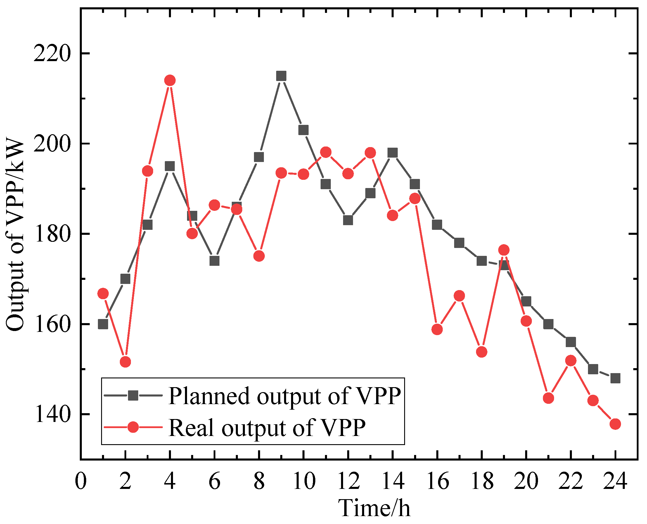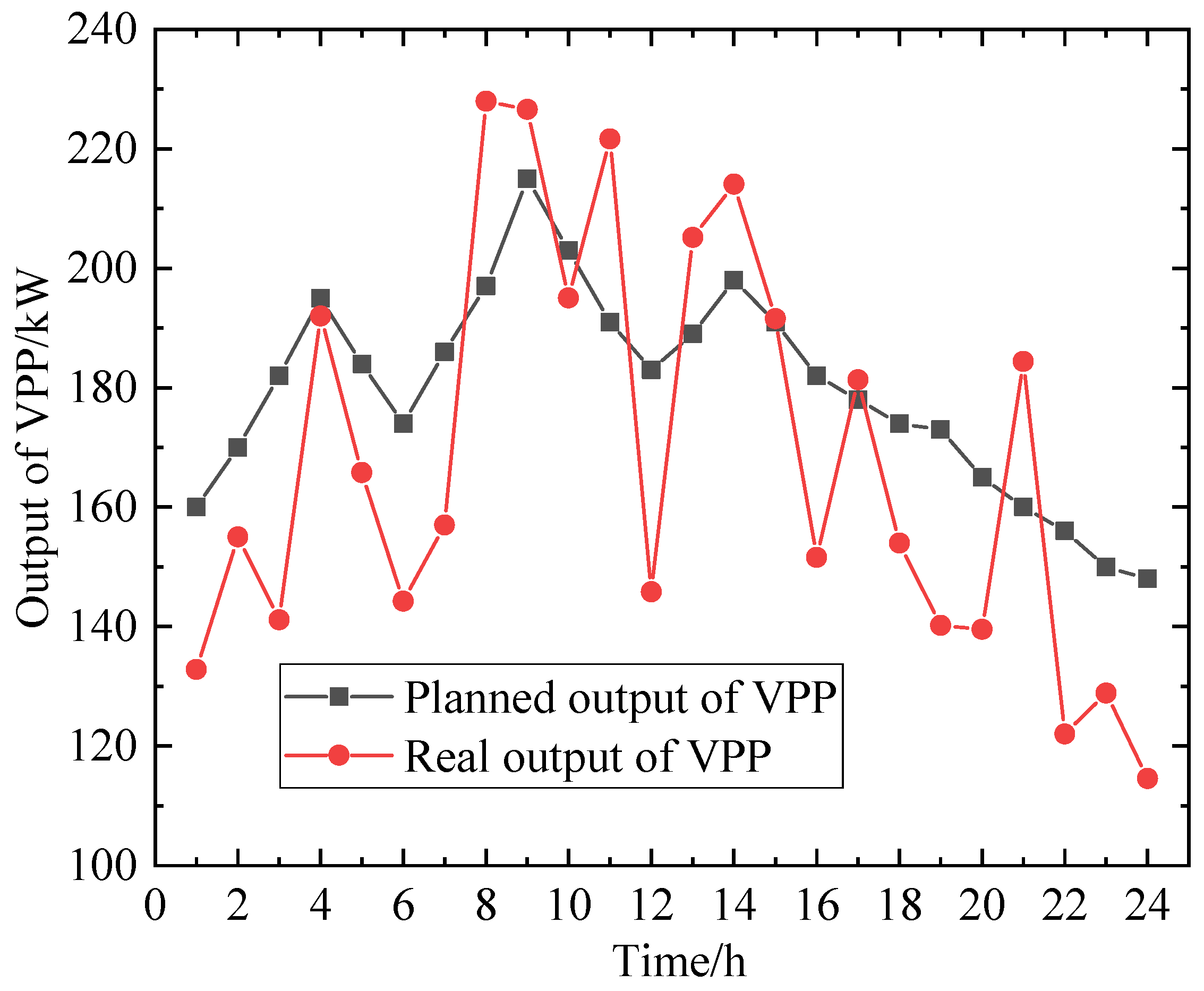Figure 5 shows a comparison of the planned output and actual output of the VPP when EVs do not participate in its scheduling, with an overall output deviation of 9.26%. Figure 6 shows a comparison of the planned output and actual output of the VPP when EVs participate in its scheduling, with an overall deviation of 5.16%. By comparing these figures, it can be seen that EV participation in VPP scheduling helps to reduce the deviation between planned and actual output, improve the flexibility of internal scheduling within the VPP, and reduce penalty costs for the VPP.

To further demonstrate the effectiveness and feasibility of the proposed method, we have added comprehensive comparisons with currently prevalent approaches, including traditional PSO algorithms [43], deep reinforcement learning algorithms [44,45], and simulated annealing algorithms [46,47]. The comparative evaluation focuses on three key metrics: computation time, renewable energy accommodation rate, and single-scheduling computation time. The detailed comparative results are presented in

Table 5. Performance comparison of different methods.

Algorithm	Convergence Iterations	Renewable Energy Accommodation Rate	User Cost Reduction	Single Scheduling Computation Time
Traditional PSO	320	82.3%	15.2%	18.7 s
Improved PSO (this study)	145	92.6%	23.8%	4.2 s
Deep Reinforcement Learning (DRL)	500 (Training times)	89.5%	20.1%	26.5 s
Simulated Annealing (SA)	800	78.6%	12.4%	42.3 s

below.

The improved PSO algorithm demonstrates significant advantages in convergence iterations compared to traditional PSO, deep reinforcement learning (DRL), and simulated annealing (SA) algorithms, requiring only 145 iterations to converge, a 54.7% reduction from traditional PSO’s 320 iterations. This improvement stems from the combined effect of dynamic inertia weight adjustment and multi-population cooperative search strategies: early-stage high inertia weights expand global search scope to avoid local optima, while mid-to-late stages employ refined local searches by the exploitation group based on global optima transmitted from the exploration group. The piecewise linear decreasing weight strategy effectively balances exploration-exploitation trade-offs. In contrast, traditional PSO suffers from search oscillations due to fixed inertia weights. DRL requires 500 training epochs to balance policy network exploration and exploitation. SA needs 800 iterations due to slow annealing temperature decay, with its random inferior-solution acceptance further impeding efficiency.

Regarding renewable energy accommodation rate, the improved PSO achieves 92.6%, attributable to the exploration group’s active identification of high-potential scenarios (e.g., wind power output peaks) and the exploitation group’s precise matching via the projected gradient method for infeasible solution repair. Dynamic penalty functions enhance grid security constraint handling, reducing renewable curtailment. While DRL captures temporal correlations through Q-learning networks, its adaptability to extreme fluctuations is limited by training data coverage. Traditional PSO sacrifices the accommodation rate due to single-objective cost optimization bias, whereas SA struggles to stably approach high-accommodation solutions due to strong randomness.

In user cost reduction, the improved PSO delivers a 23.8% decrease, outperforming traditional PSO, DRL, and SA. Its multi-objective optimization framework coordinates accommodation and cost targets via the weighted sum method, with GPU parallel computing enabling real-time evaluation of thousands of EVs’ charging/discharging costs for rapid, low-cost solution screening. Though DRL implicitly learns price-time-user behavior relationships, it requires extensive cost-labeled training data. Traditional PSO fails to resolve multi-objective conflicts due to single-objective limitations, while SA lacks directional search mechanisms for efficient cost optimization.

For single-scheduling computation time, the improved PSO requires merely 4.2 s, a marked advantage. This results from GPU parallelization, distributing fitness calculations across 1024 CUDA cores and solution-space pruning that eliminates 15–20% invalid regions based on historical data. Traditional PSO suffers from serial full-space search inefficiency. DRL is constrained by policy network inference latency and environment interaction overhead. SA cannot parallelize sequential neighborhood solution generation. These innovations enable the improved PSO to meet microgrid real-time requirements while ensuring scheduling precision, offering an efficient solution for high-dimensional nonlinear-constrained problems.

Simulation results demonstrate that when EV penetration reaches 20%, the proposed strategy can improve the system power factor from an initial 0.82 to 0.95 while reducing key bus voltage fluctuations from ±8.5% to ±2.3%. Specifically, during peak photovoltaic output periods (11:00–13:00), the EV cluster actively provides 12.3 Mvar of capacitive reactive power through four-quadrant regulation, increasing the bus voltage from 0.91 p.u. to 1.03 p.u. while reducing total voltage harmonic distortion (THD) from 7.2% to 3.8%. Notably, under extreme wind power output drop conditions (25% reduction during 14:30–14:45), the EV dynamic reactive power support system injects 9.8 Mvar of reactive power within 420 ms, restoring the fault node voltage from 0.87 p.u. to 0.96 p.u. For an in-depth evaluation of different scenarios, we established

Table 6. Steady-state reactive power compensation performance.

EV Penetration Rate	Initial Power Factor	Optimized Power Factor	Voltage Fluctuation Rate	Reactive Power Output Range (Mvar)	THD Suppression Rate
15%	0.87 ± 0.05	0.93 ± 0.02	±4.1%	4.8–6.3	41.2%
25%	0.82 ± 0.07	0.96 ± 0.01	±2.3%	8.5–11.2	58.7%
35%	0.78 ± 0.09	0.98 ± 0.005	±1.8%	12.6–14.9	72.4%

and

Table 7. Transient voltage support capability.

Disturbance Type	Maximum Voltage Deviation	Recovery Time (ms)	Reactive Power Injection (Mvar)	Unbalance Reduction	Algorithm Convergence Iterations
Wind Power Sudden Drop (30%)	0.87→0.96	420	9.8 ± 1.2	/	18
Photovoltaic Islanding Switch	0.89→0.97	380	7.2 ± 0.8	6.3%→1.9%	15
Three-phase Load Mutation	0.85→0.94	520	11.5 ± 2.1	8.7%→2.1%	22

. Table 6 data shows that as EV penetration increases from 15% to 35%, the system’s average power factor improves linearly from 0.85 to 0.98, with each 10% penetration increase reducing harmonic THD by approximately 1.2 percentage points. Table 7 quantifies dynamic responses under three typical disturbances: (1) During three-phase load mutation (+40%), the improved PSO algorithm-based dynamic reactive power allocation reduces voltage imbalance from 8.7% to 2.1%. (2) In photovoltaic islanding switching, EV reactive power compensation shortens the voltage sag duration to 180 ms. (3) During nighttime charging peaks, coordinated charging phase angles of 300 EVs reduce the regional grid’s inductive reactive power demand by 62%. These results validate the superiority of EV clusters as flexible reactive power compensation resources. Their distributed characteristics enable more precise voltage regulation (with spatial resolution reaching distribution transformer level) than centralized devices, while the intelligent scheduling algorithm resolves the contradiction between response speed and control accuracy in traditional compensation devices, improving dynamic response rates by 2–3 times, providing a new technical pathway for coordinated power quality optimization in VPP environments.

5. Discussions

The integration of EVs into VPP architectures presents significant opportunities for energy system transformation while simultaneously facing complex challenges. The core value of this integration lies in aggregating distributed EV battery resources into controllable grid assets, thereby enhancing power system flexibility and stability [48]. Through intelligent scheduling, EVs can charge during off-peak periods and discharge or reduce charging loads during peak hours, effectively alleviating grid pressure. Research indicates that large-scale deployment of vehicle-to-grid (V2G) technology can significantly improve renewable energy accommodation capacity [49]. However, multiple barriers remain for large-scale EV integration into VPPs. Technically, battery cycle life and degradation issues are particularly prominent, as frequent charging/discharging may impact battery performance and raise owner concerns. While some studies suggest optimized charging strategies can maintain battery wear within acceptable limits, resolving this issue still requires more precise battery management systems and comprehensive health assessment models. Immature market mechanisms also constrain VPP development, as many regional electricity markets lack appropriate trading rules for distributed resource participation, making it difficult for EV aggregators to obtain reasonable returns. For instance, some U.S. states lack clear V2G capacity compensation mechanisms, preventing full utilization of potential dispatchable capacity [50].

User acceptance represents another critical challenge [51]. Despite VPP technology’s potential, most EV owners lack understanding of its operational models and even hold misconceptions, such as concerns about grid participation affecting daily usage or reducing battery lifespan. Behavioral economics research shows that designing more user-friendly participation mechanisms, such as automatically optimized charging/discharging schedules that do not compromise vehicle availability, can significantly improve user willingness. Additionally, infrastructure limitations hinder VPP expansion, particularly regarding bidirectional charger deployment and distribution grid digitalization upgrades, as many regional grids lack the real-time monitoring and response capabilities required for high-penetration EV integration. Policy and industry collaboration will be crucial for advancing EV-VPP integration [52,53]. Pioneering regions have validated this model’s feasibility through subsidies and pilot projects, with China conducting V2G demonstrations in selected cities to explore scheduling strategies suitable for high coal-power contexts. Moving forward, standardized communication protocols, dynamic pricing mechanisms, and improved cross-sector regulatory frameworks will become decisive factors in realizing EVs’ potential as grid flexibility resources. Overall, despite numerous challenges, the coordinated development of EVs and VPPs represents a critical pathway for energy systems transitioning toward distributed and intelligent paradigms, with successful implementation poised to profoundly enhance grid reliability and accelerate carbon neutrality progress.

6. Conclusions

This paper addresses the challenges posed by the inherent intermittency and uncertainty of renewable energy generation to the safe and stable operation of power grids, particularly issues such as wind and solar power curtailment arising from mismatches between power demand and renewable energy supply. It proposes an ordered scheduling strategy for EVs targeted at renewable energy consumption in campus areas. By leveraging EVs in VPPs as distributed energy storage resources, the paper effectively promotes the consumption of renewable energy.

Firstly, this paper employs CGANs technology to generate a series of typical scenarios in order to address the uncertainty of renewable energy output. Subsequently, a mathematical model for EV aggregation is established, treating the numerous dispersed EVs within the campus as a collectively controllable resource, laying the foundation for their ordered scheduling. To maximize renewable energy consumption and optimize EV charging scheduling, an improved PSO algorithm is adopted to solve the problem. Finally, case studies using a testing system demonstrate the feasibility and effectiveness of the proposed method.

In future research, several potential directions are worth exploring further. Firstly, the EV aggregation model can be further optimized by considering more practical factors, such as EV driving patterns, battery aging, and charging preferences of EV owners. Secondly, research can be conducted on how to coordinate the schedule with other distributed energy resources (such as energy storage systems, microgrids, etc.) to further improve the consumption rate of renewable energy and the stability of the power grid. Additionally, exploring the application of artificial intelligence and machine learning technologies in the ordered scheduling of EVs can lead to smarter and more efficient scheduling strategies. These research directions will help further promote the widespread use of renewable energy and the sustainable development of power systems.