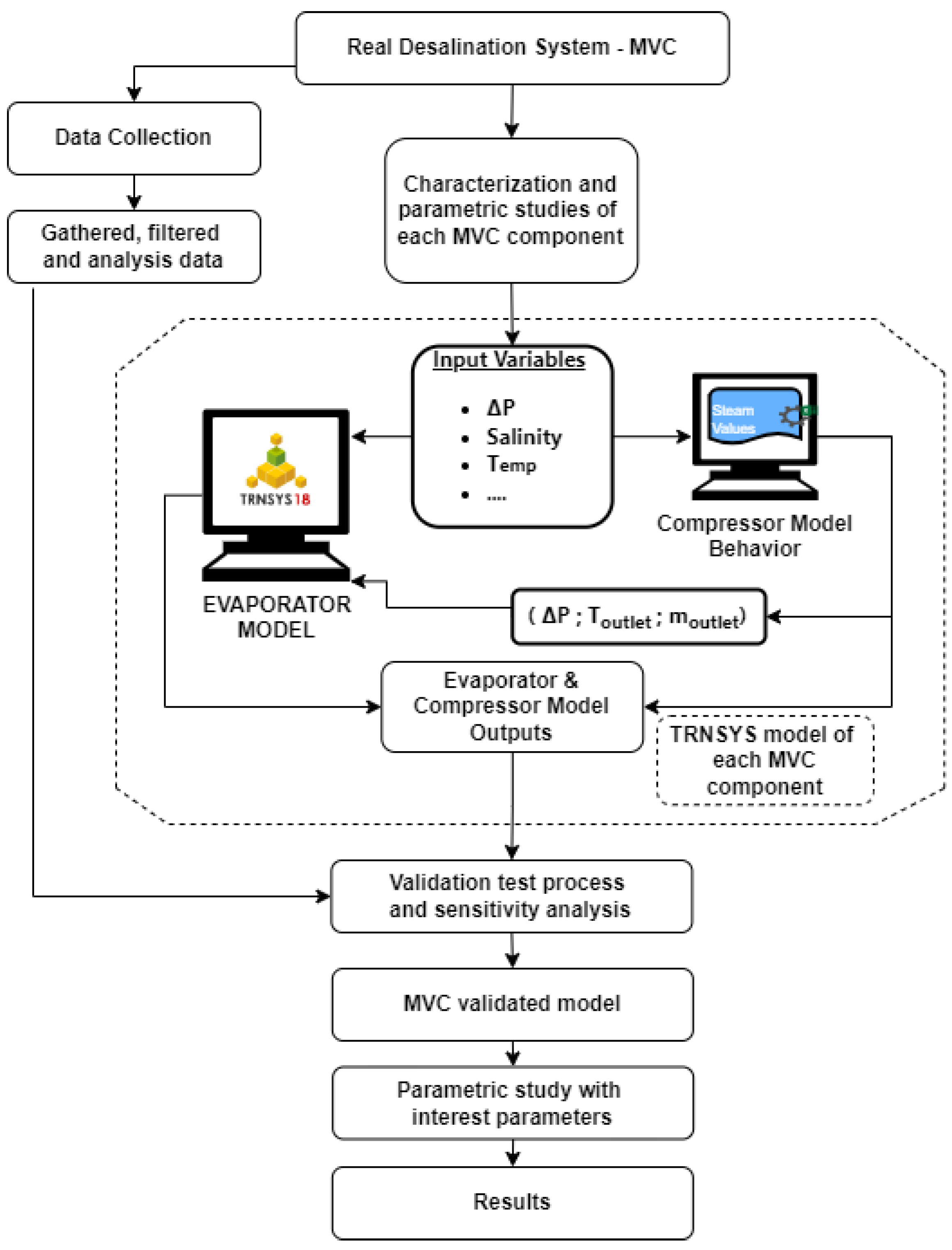
This contribution proposes a feasible model of an MVC system with TRNSYS software [
26], considering constraints observed from a real life experimental plant and validating the model with real measured values from that same tested MVC experimental facility [
31]. Parametric studies can be generated in this model with different operating conditions, estimating which variable affects the most to the final outcome of the system, but this contribution focuses on its validation only. The methodology followed is shown schematically in
Figure 3. The process starts by understanding the relationships between the components of the real MVC plant, including their mass and energy balances, and determining the availability of the necessary variables for these balances. After that, data from the MVC experimental plant in operation are gathered, selected and filtered. This data will be used to validate and verify the reliability of the model created. In parallel, each element in the MVC desalination system is independently characterized, calculated and connected to create a model in
Section 4.1. The proposed model is based on the combined calculation of the two main components of the MVC: the compressor and the evaporator. These components’ models are explained in the following
Section 4.2 and
Section 4.3.
The compressor is designed to generate vacuum pressures up to −0.5 barG (51.325 kPa absolute pressure), where the saturation temperature inside the evaporator reaches °C. The outlet temperature of the compressor has a manufacturer’s limit set at °C and should be greater than °C to take advantage of the latent heat from the superheated vapour. For the evaporator, the concentration stage lasts 4 min (240 s), while the time for the rejection of the brine is between 3 and 4 s long and refilling of the evaporator lasts 10 s.
4.3. Description of the Modelled Evaporator in MVC
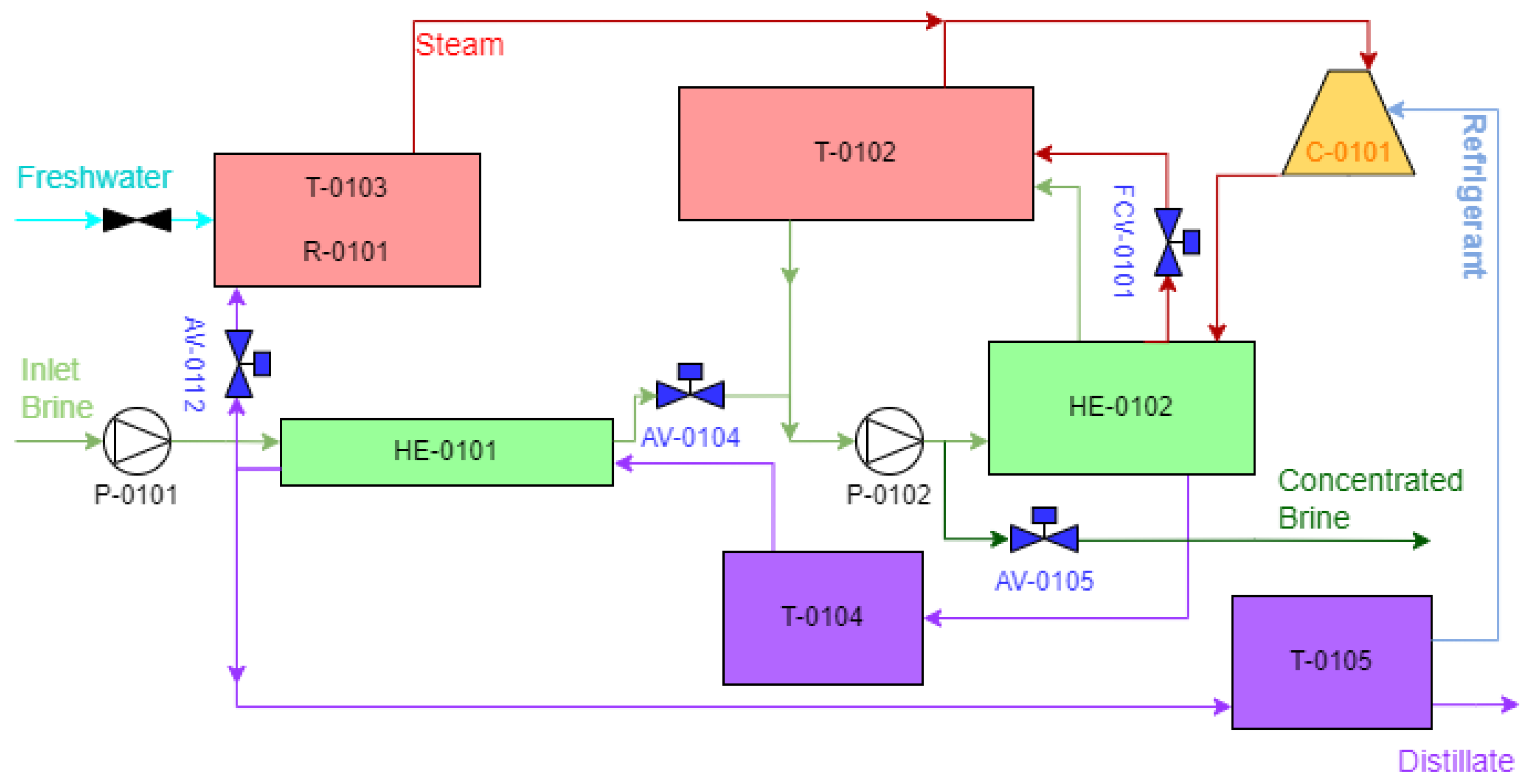
Concerning the evaporator, note that both heat exchanger and the flash tank from the real experimental plant are considered as a unique element in the modelled evaporator. It simplifies energy and mass balances, and it does not affect either input or output flow rates in the evaporator. The mission of the flash tank is separating the steam created in the evaporator from the rest of the liquid brine still remaining in the heat exchanger. The modelled evaporator will operate during heating and concentration stages only; the filling stage is discarded from the model since there are no means for validating its results with real values from the experimental facility. As a result, the evaporator experiment tests two different situations along the MVC’s operation: a first phase, where the internal energy of the evaporator increases until saturation conditions are reached, and a second phase, where the brine is both distilled and concentrated under previously calculated compressor operating conditions, Calleja-Cayón [
24].
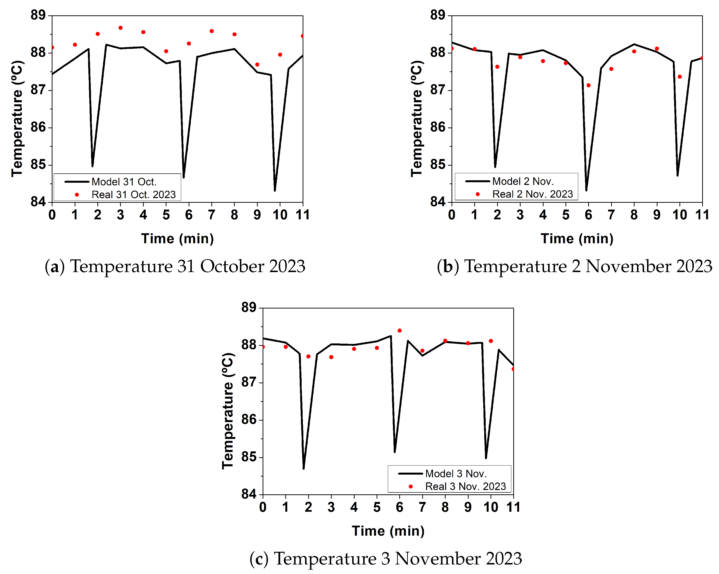
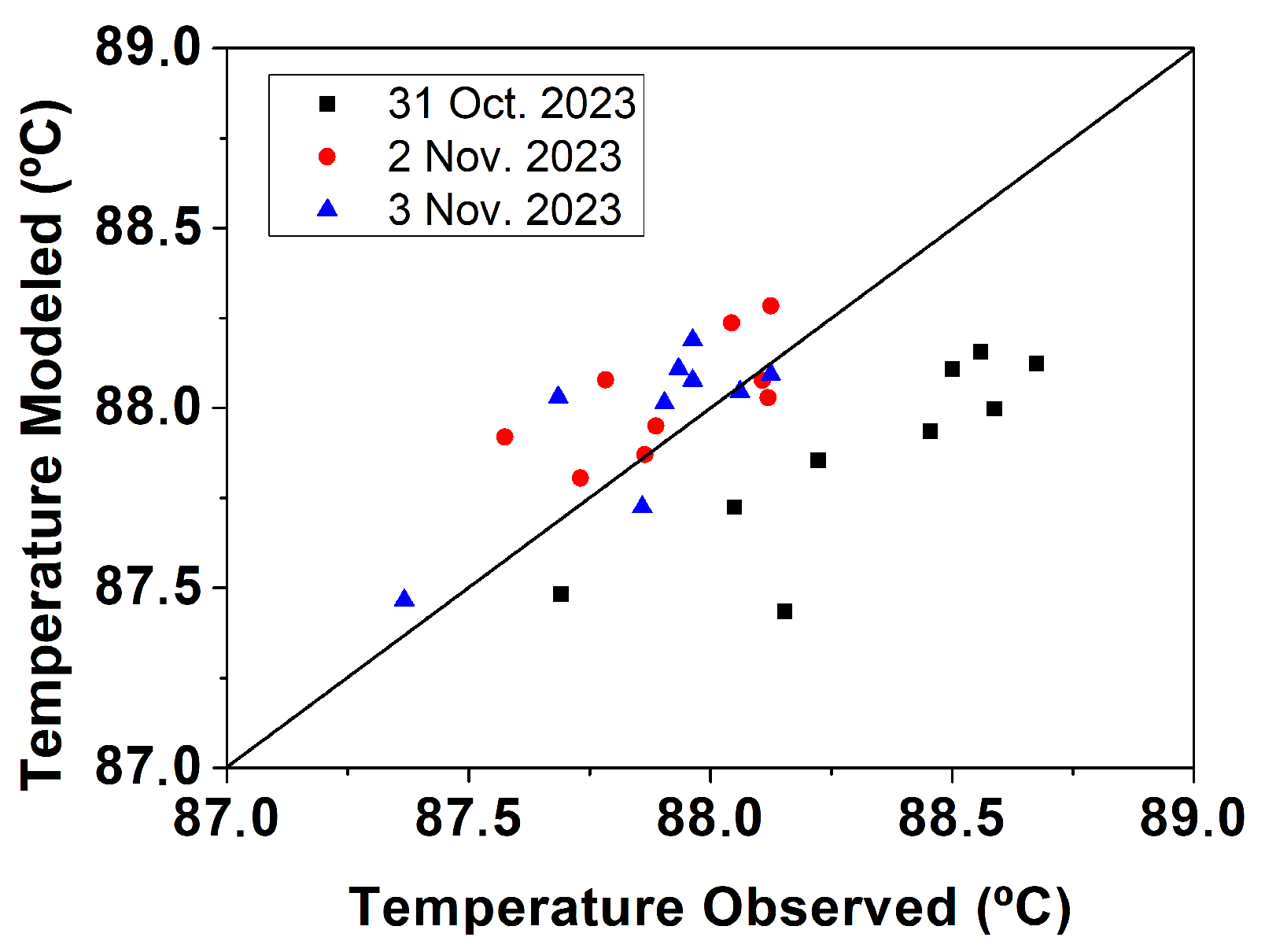
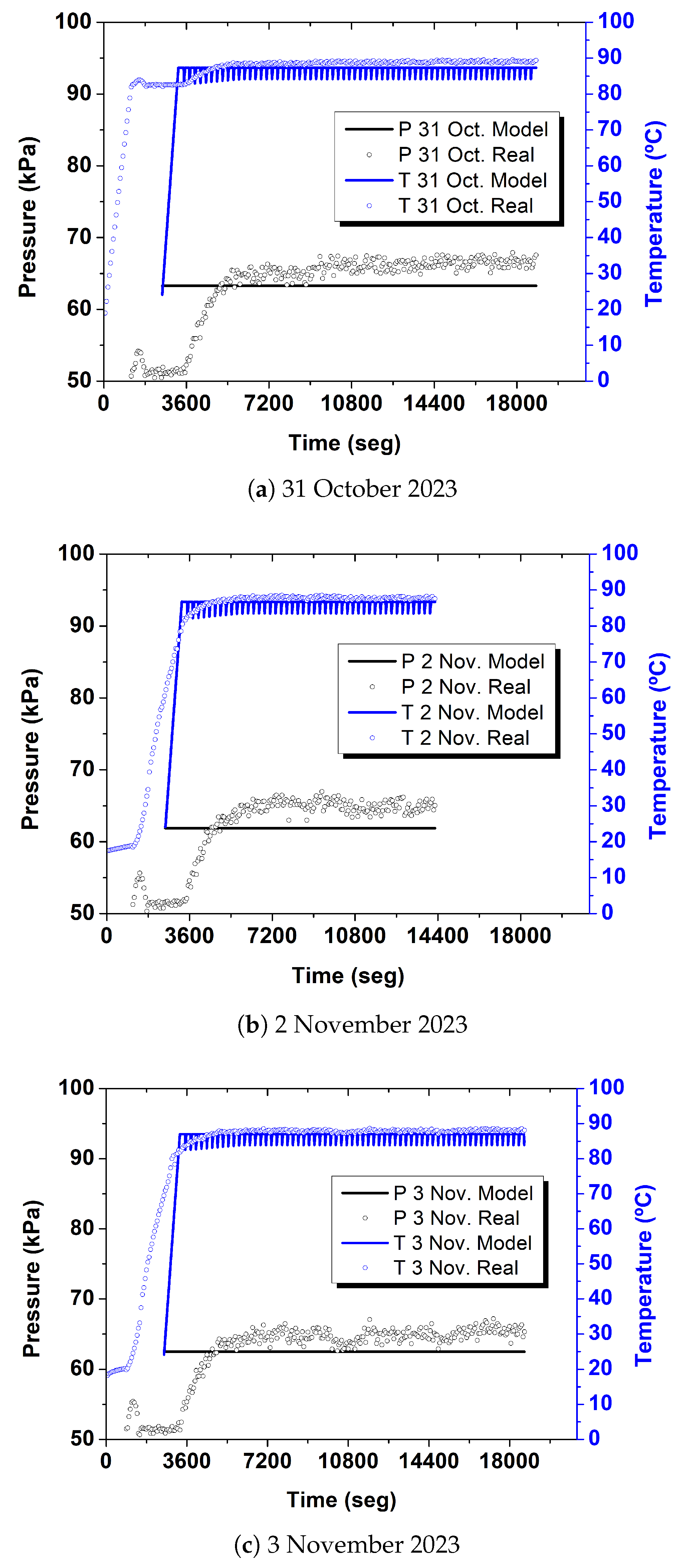
The MVC model and its evaporator are validated with the data registered at the LIFE Desirows’ MVC facility [
31]. In these two stages, heating and concentration, different situations can occur depending on both the evaporation process’s time interval and the sensors signals reaching the evaporator. Each situation is called a ‘case’, and each case uses the continuity equations with different input values depending on their incoming and outgoing streams. Each ‘case’ depends on the opening and closing of each of the valves connected to the evaporator, but especially of the relative time within each cycle. This opening and closing of valves generates different situations in the mass and energy balance, reinforcing the importance of a correct definition of each ‘case’.
Figure 6 shows a graphical diagram of the steps followed for selecting each ‘case’.
When the MVC begins, the compressor and electric heater are activated, but steam production will be zero until saturation conditions are reached inside the evaporator. This period is called the “Heating Stage” or ‘Case 0’.
Once saturation conditions are reached, the “Concentration Stage” begins, producing distillate (steam) and concentrating the brine inside the evaporator, depending on different situations (‘Cases 1–8’).
In the concentration stage, the model of the evaporator requires two different values for selecting the proper ‘case’: the first one is to know in which moment of the concentration period the time-step is located,
Table 2, and second, in case of reaching the maximum or minimum levels, the model decides to open or close valves. For the model, the ‘level’ is calculated with the amount of brine inside the vacuum tank,
Table 2, while the real MVC facility disposes of two separate sensors measuring each level.
The equations used to update the evaporator conditions in ‘Case 0’, heated by the auxiliary heating element, are the following:
where
is the specific heat of the cold source (brine),
is the temperature inside the evaporator on the previous time-step,
the tuning factor,
is the mass of brine inside the evaporator (initial mass of 79 kg),
is the heat absorbed from the hot source after losses and
is the temperature of the evaporator after absorbing that amount of energy. The value of
is constant for each pressure and compares the values of
h under saturated liquid conditions.
For the initial time-step, trnsys reads the list of ‘parameters’ and ‘inputs’ introduced in the evaporator’s type (atmospheric conditions), which are meant to be the initial values for the modelling stage, while for the next time-steps, the model will read the value calculated on the previous time-step as the new input value. ‘Case 0’ lasts as long as is lower than the product of the initial mass () and the specific enthalpy of the saturated liquid () at these pressure conditions, when saturation conditions are achieved and evaporation can start. Once the heating stage is finished, it is time for the concentration stage, where (i) brine inside the evaporator is distilled and concentrated, (ii) the concentrated brine is periodically removed, and (iii) once the removal is finished, new inlet brine is introduced to the evaporator, restarting (i). In the model, these situations correspond to Cases 1 to 8:
Case 1: Brine concentration. AV-0104, AV-0105 and FCV-0101 OFF.
Case 2: Brine concentration with evacuation of concentrated brine. AV-0105 ON, AV-0104 and FCV-0101 OFF.
Case 3: Brine concentration with refill of brine. AV-0104 ON, AV-0105 and FCV-0101 OFF.
Case 4: Brine concentration with evacuation and refill simultaneously. AV-0104 and AV-0105 ON, FCV-0101 OFF.
Case 5: Brine concentration with superheated steam input. AV-0104 and AV-0105 OFF, FCV-0101 ON.
Case 6: Brine concentration with evacuation and superheated steam input. AV-0104 OFF, AV-0105 and FCV-0101 ON.
Case 7: Brine concentration with refill and superheated steam input. AV-0105 OFF, AV-0104 and FCV-0101 ON.
Case 8: Brine concentration with evacuation, refill, and superheated steam input simultaneously. AV-0104, AV-0105 and FCV-0101 ON.
For each time-step, with a duration of
, the model starts by reading the variables responsible for the selection of these cases. The parameters used to select each case, listed in
Table 2, are LSH-0102, LSL-0102, FCV valve, concentration time, rejection time and filling time.
During concentration stage, Cases 1–8, the equations used for updating the evaporator’s conditions are divided into two groups: those related to the hot source and those related to the treated brine.
The hot source equation, Equation (
4), refers to the heat flux from the compressor. The inlet brine, outlet concentrated brine, and superheated steam flow rates from valve FCV-0101 depend on the opening or closing of the valves AV-0104, AV-0105 and FCV-0101. During the concentration stage and their Cases 1–8, energy and mass balances are applied to the evaporator, Equation (5), and the new evaporator condition is calculated with Equation (
6). Subsequently, the generated steam, Equation (
7); the new mass in the evaporator, Equation (
8); and the new properties, Equation (
3), are calculated.
where subscripts brine, cbrine and steam correspond to the inlet and outlet fluxes of brine, concentrated brine and steam, and the mass and enthalpy depend on the opening or closing of valves AV-0104, AV-0105 and FCV-0101. The equations shown in Equation (5) unify the heat exchanger and flash tank in a single set of equations due the interconnection of both flash tank and heat exchanger. Attempting to model both appliances independently, flash tank and heat exchanger, would require introducing artificial internal variables whose uncertainty would exceed that of this simplified approach without any improvement.
The inlet and outlet mass flow through each of the valves mentioned above for Equation (5), if open, and are calculated using the nozzle equation for each time-step.
To calculate the steam properties, the
found in the TRNSYS library has been used. However, to calculate the brine enthalpy, a new
has been generated that uses the correlation of the isobaric specific heat (
) of seawater, Equations (
10) and (
11), created by Jamieson in 1969 [
33], valid for the temperature range of 0–
°C and salinities of 0–180 g/kg and matching the experimental facility’s requirements.
being
Regarding
of the steam, another formula based on the specific enthalpy (
h) and temperatures of the steam and saturation conditions is used. Using TRNSYS Type58, the enthalpy and temperature values of both the saturated steam and the compressor’s outlet can be achieved. These two sets of outputs allow the specific heat capacity value to be calculated using the following correlation:
The value of will be considered the same for both the inlet and outlet of the compressor, simplifying the number of equations and with an accumulative error lower than ( kJ/kg·K and kJ/kg·K), prioritizing the use of Type58 for obtaining over .
The final relevant output expected from a desalination plant is the final salinity of the waste product, Equation (
13). Since the experimental plant measures the conductivity of both the inlet brine and the final concentrated brine each day of operation, a linear conversion from conductivity to salinity is used to validate the model output values, Equation (
14).
Regarding evaporator operation, it starts with the heating stage. Considering the initial amount of brine inside the evaporator is between and , it lasts until the total mass of brine inside it reaches saturation conditions. It then continues with the cycle of cases for the concentration stage, which will be on repeat until the desalination plant stops its operation.


 ,
, 


