Abstract
Water injection is widely recognized as one of the most important operational approaches for enhanced oil recovery in oilfields. However, this process faces significant challenges due to the formation of sulfate and carbonate mineral scales caused by high salinity in both injected water and formation water. To address this issue, the use of mineral scale inhibitors has emerged as a valuable solution. In this study, we evaluated the performance of seven machine learning algorithms (Gradient Boosting Machine; k-Nearest Neighbors; Decision Tree; Random Forest; Linear Regression; Neural Network; and Gaussian Process Regression) to predict inhibitor efficiency. The models were trained on a comprehensive dataset of 661 samples (432 for training; 229 for testing) with 66 features including temperature; concentrations of various ions (sodium; calcium, magnesium; barium; strontium; chloride; sulfate; bicarbonate; carbonate, etc.), and inhibitor dosage levels (DTPMP, PPCA, PBTC, EDTMP, BTCA, etc.). The results showed that GPR achieved the highest prediction accuracy with R2 = 0.9608, followed by Neural Network (R2 = 0.9230) and Random Forest (R2 = 0.8822). These findings demonstrate the potential of machine learning approaches for optimizing scale inhibitor performance in oilfield operations
1. Introduction
The injection process is one of the key operations in the oil industry, particularly for enhanced oil recovery (EOR) [1]. While this method is highly effective in improving extraction efficiency, it faces challenges such as the formation of mineral deposits [2]. In simple terms, formation water in oil fields contains dissolved minerals like sodium, barium, calcium, sulfate, bicarbonate, and chloride. When this water is mixed with injection water, the equilibrium of this system can be disrupted based on the concentration of ions and their intermolecular reactions. Under certain operational conditions, the system may become supersaturated, leading to mineral scale formation [3,4,5].
One of the main strategies to manage and prevent this issue is the use of scale inhibitors [6,7,8,9,10]. These chemicals help control mineral deposition, though their effectiveness can vary depending on different factors. Using the correct amount of antiscale chemicals is critical because too little or too much can cause pipeline blockages [11].
Extensive research has evaluated the effectiveness of mineral scale inhibitors at optimal concentrations. Yang et al. (2025) [12] developed an eco-friendly scale inhibitor called PEBMAA-EDA, which achieved 83.61% effectiveness at low concentrations, making it a better alternative to traditional methods. Their research showed it works by chelating minerals, distorting crystal structures, and preventing scale formation through adsorption [12]. Hu et al. (2025) [13] studied a new water-soluble copolymer (Acrylic Acid-(N-Acryloyloxyethyl Pyrrolidone-2-Carboxylic Acid Ethyl Ester)) made from acrylic acid and a novel monomer (N-Acryloyloxyethyl pyrrolidone-2-carboxylic acid ethyl ester). Their research showed that increasing the carboxyl-to-ethylene oxide ratio improves scale prevention by distorting CaCO3 crystals and enhancing adhesion to surfaces. Zhang et al. (2019) [14] investigated how dissolved iron (Fe2+) affects scale inhibitors in oilfield operations, using a specialized oxygen-free setup to prevent iron oxidation. Their findings revealed that Fe2+ reduces inhibitor effectiveness, but citrate—unlike Ethylenediaminetetraacetic acid (EDTA)—can help restore performance under controlled pH and temperature conditions.
In oil recovery, especially during waterflooding, using scale inhibitors is essential to prevent mineral buildup. Since waterflooding plays a key role in oil production, many researchers have studied how to best use these inhibitors to solve this common problem. Khormali et al. (2021) [15] studied the formation of calcium and strontium sulfate scales under different reservoir conditions. They tested five commercial inhibitors and developed a new inhibitor (DPAAI), which showed 94% efficiency even at high temperatures (150 °C) and significantly improved squeeze lifetime (85% longer than conventional inhibitors). Khormali et al. (2018) [16], in another study, addressed calcium sulfate scaling during waterflooding caused by incompatible injection and formation waters. They developed a novel phosphonate-based inhibitor mixture showing over 90% efficiency across all tested reservoir temperatures (60–120 °C) and water mixing ratios (10–90% formation water). Zakaria et al. (2020) [17] investigated the use of three cost-effective, phosphonate-based scale inhibitors derived from expired pharmaceuticals—zoledronic acid (ZDA), alendronic acid (ADA), and pamidronic acid (PDA)—for controlling oilfield scale in Egyptian reservoirs. Their study combined theoretical predictions (using OLI ScaleChem software) and experimental tests to evaluate scaling risks and inhibitor performance under both ambient (77 °F, 14.7 psi) and reservoir conditions (260 °F, 3600 psi) [17].
Given the proven effectiveness of machine learning techniques in oilfield operations [18,19,20,21,22], this study investigates the prediction of mineral scale inhibitor efficiency using multiple machine learning algorithms. Previous studies in mineral scale inhibitors have primarily relied on experimental methods, with no machine learning-based predictive model developed for this application to date. In this work, we present the first data-driven framework using seven machine learning algorithms (including Gaussian Process Regression (GPR), neural networks, and random forests) trained on a comprehensive dataset of 661 laboratory samples to predict inhibitor efficiency. A key innovation is the introduction of GPR for this purpose, which effectively handles high-dimensional nonlinearity through feature interaction analysis. This approach offers a significant advancement in scale management for the oil industry by enabling more accurate, computationally efficient predictions. This study specifically evaluates Gaussian Process Regression against six other widely used algorithms and provides valuable insights for future research.
2. Data and Methods
2.1. Algorithms Used in This Study
Given the critical role of machine learning in predictive chemical processes, this study evaluates seven distinct algorithms: Decision Tree (DT), Random Forest (RF), Artificial Neural Network (ANN), k-Nearest Neighbors (KNN), Gaussian Process Regression (GPR), Gradient Boosting Machine (GBM), and Linear Regression (LR). These models predict inhibitor efficiency based on formation/injection water salinity, inhibitor concentration, and temperature. The unified flowchart below outlines their implementation. We used MATLAB software (R2023b; University of Regina, Regina, Canada) for this work.
2.1.1. Data Preparation (Common to All Models in This Study)
- Input structuring:
- -
- Features (‘X’): Transpose raw matrix ‘D’ to *N × M* (N = samples, M = features);
- -
- Target (‘T’): Convert ‘S’ to column vector, clip to experimental range (e.g., [11%, 98%] for inhibition efficiency).
- Train-Test split:
Based on the attached database (see the supplementary Excel file), the following division was used in the study:
- ▪
- Training: First 432 samples (≈65% for model development);
- ▪
- Test: Remaining samples (≈35% for unbiased evaluation).
Therefore, the validation criterion in this study is based on the Hold-Out method. However, the data selection for the training and test sets was not random. Instead, for each specific solution containing inhibitors and mineral ions, some experimental data were used to train the algorithm, while the remaining data were reserved for testing. This ensures that the algorithm is evaluated on completely unseen data, allowing its predictive performance to be objectively assessed. The Supplementary Excel file is structured with a clear division: the training dataset (first section), containing samples used for model development, is followed by the test dataset, which includes unseen data from the same solutions for evaluation.
2.1.2. Model-Specific Hyperparameter Tuning
- Decision Tree: Minimum leaf size = [1, 2, 4, …, 32]; Optimization Criterion: Minimal MAE.
A range of ‘MinLeafSize’ values from 1 to 32 was tested to evaluate its effect on the performance of the decision tree model. This parameter controls the minimum number of observations required in a leaf node. Smaller values allow the tree to grow deeper and capture more detail from the training data, which can lead to overfitting. On the other hand, larger values result in a shallower tree that may miss important patterns, leading to underfitting. By selecting the ‘MinLeafSize’ that yielded the lowest Mean Absolute Error (MAE) on the test data, the model achieves a good balance between accuracy and generalization.
- Random Forest: Number of Trees = [10, 50, 100, …, 500]; Optimization Criterion: Minimal MAE + OOB error.
A range of tree numbers from 10 to 500 was tested to examine the effect of the number of trees on the performance of the Random Forest model. Using fewer trees (e.g., 10 or 50) can reduce training time but may lead to less stable and less accurate predictions due to higher variance. Increasing the number of trees generally improves performance and stability by averaging out the errors of individual trees. However, beyond a certain point (e.g., 200 or 500 trees), the improvement becomes minimal, and training becomes more computationally expensive. The optimal number of trees was selected based on the lowest MAE, providing a good balance between accuracy and computational efficiency.
- Neural Network: Hidden Layer Size = [5, 10, …, 20]; Optimization Criterion: Minimal MAE
A range of 5 to 20 neurons for a single hidden layer was selected as a balanced choice for medium-sized data (432 training samples). More complex architectures were avoided to reduce the risk of overfitting. The activation function used in the hidden layer is tansig (hyperbolic tangent sigmoid), and in the output layer is purelin (linear function). This choice was made because the output values fall within a specific range, and these functions are well suited for such cases.
- KNN: K = 1 to 50; Optimization Criterion: Minimal MAE
A sensitivity analysis was performed by testing K values from 1 to 50 to find the optimal number of neighbors for the KNN model. The number of neighbors directly affects the model’s bias-variance tradeoff. A smaller K can lead to high variance (overfitting), while a larger K can cause high bias (underfitting). Therefore, the K value that resulted in the lowest Mean Absolute Error (MAE) on the test data was selected as the optimal number of neighbors. This approach helps ensure that the model is both accurate and generalizable.
- Gaussian Process: Length Scale, Sigma (log-scale); Optimization Criterion: Minimal MAE + R2
In this study, we performed a sensitivity analysis on the two main hyperparameters of the squared exponential kernel in the Gaussian Process Regression (GPR) model:
- ▪
- Length Scale: Controls how far two inputs need to be for their outputs to be considered uncorrelated;
- ▪
- Sigma (Signal Standard Deviation): Represents the signal variance, determining the overall scale of variation in predictions.
We tested a wide range of values for both parameters using a logarithmic scale:
length_scale_values = logspace (−2, 2, 20); % Tested length scale values
sigma_values = logspace (−2, 1, 20); % Tested sigma values
This created 20 points per parameter that were equally spaced in log-space, providing balanced coverage of the possible parameter ranges while maintaining computational efficiency.
We employed logarithmic spacing for our parameter optimization based on several important considerations:
- Efficiency in Exploration:
Logarithmic spacing allows us to efficiently examine parameters that can vary across orders of magnitude. Since both length scale and sigma parameters can have significant impacts even at small values, this approach ensures we do not miss important variations in the low-value ranges that linear spacing might overlook.
- 2.
- Computational Advantages:
The logarithmic approach provides several practical benefits:
- ▪
- Fewer total test points needed compared to linear spacing;
- ▪
- Better coverage of the parameter space;
- ▪
- More likely to find the true optimum;
- ▪
- Standard practice in machine learning optimization.
- Gradient Boosting: NumTrees, LearnRate, MaxDepth; Optimization Criterion: Minimal MAE + feature importance.
The ranges selected for hyperparameters were based on:
- Number of Trees (50–200): Common range for ensemble methods (too few→underfitting, too many→overfitting);
- Learning Rates (0.01–0.2): Standard GBM practice (lower rates need more trees but generalize better);
- Max Depth (2–4 via MinLeafSize): Controls complexity (deeper trees risk overfitting)
- Linear Regression: None (closed-form solution)
2.1.3. Model Training & Validation
- -
- Common steps:
- Train: Fit model to training data with optimal hyperparameters;
- Predict: Generate test predictions, clip to physical bounds;
- Evaluate: Compute metrics (MAE and R2).
2.1.4. Performance Comparison
- -
- Visualization: Overlay predicted vs. actual plots for all models (subplots);
- -
- Metric table: Compare MAE and R2;
- -
- Critical analysis:
- ○
- Interpretability: Decision trees > linear regression > others;
- ○
- Flexibility: GPR/NN > ensemble methods > linear models;
- ○
- Computation: GPR/NN > RF/GBM > others.
2.2. Data Collection
In this study, approximately 661 samples were collected to evaluate and predict the performance and efficiency of mineral scale inhibitors in oilfields. The dataset includes 66 features, such as temperature, the concentration of cations and anions in formation and injected water, and inhibitor dosage. Key cations in the injected and formation water include calcium, barium, strontium, iron, sodium, potassium, and lithium, while major anions comprise chloride, sulfate, carbonate, and bicarbonate. The concentrations of these ions can significantly influence the effectiveness of scale inhibitors.
The study examined the performance of various mineral scale inhibitors in oilfield systems, including EDTMP, HDTMP, DTPMP, PBTC, ATMP, HEDP, PPCA, PPNMP, and several inhibitor mixtures (e.g., mixtures of H5P3O10, C2H7NO, (CH3) PO(OH)2, and C16H32O6; (CH3)PO(OH)2, K4P2O7, C2H7NO, and CH6NO3P, etc.). Table 1 provides detailed information on the collected dataset, including temperature conditions, inhibitor concentration ranges, mineral concentrations in formation and injection water, and the target mineral scales. The primary scales investigated were calcium sulfate, calcium carbonate, barium sulfate, and strontium sulfate.

Table 1.
Input features and target variable used in machine learning models for scale inhibitor efficiency prediction.
Data were collected from reliable international references that explicitly reported the concentrations of mineral ions in both formation and injected water, along with inhibitor dosages and operational temperatures. This ensured high-quality training data for machine learning algorithms to accurately predict scale inhibitor performance. Temperature was another critical variable, with precise details extracted from references to enhance model training and testing. The complete dataset used in this study is available in the Supplementary Material.
In this study, feature importance was calculated using the Out-of-Bag (OOB) Permuted Predictor Importance method, a robust technique for evaluating feature contributions to predictive performance [30,31]. One key advantage of random forests is their ability to estimate predictor importance through permutation of OOB observations across the ensemble of trees [30,31,32,33]. This approach was selected because it provides reliable importance measures while maintaining the model’s predictive accuracy and handling high-dimensional data effectively. This study also analyzes feature selection based on correlation matrices.
3. Results and Discussion
This study evaluates the performance of mineral scale inhibitors in oilfield systems using machine learning algorithms trained on an experimental dataset comprising 661 samples (432 training, 229 testing) with 66 features, including temperature, ionic concentrations (Na+, Ca2+, Mg2+, Cl−, SO42−, HCO3−, etc.) in formation/injection waters, and inhibitor dosages (DTPMP, PPCA, PBTC, EDTMP, BTCA, etc.). Seven algorithms were compared: Neural Network (NN), Decision Tree (DT), K-Nearest Neighbors (KNN), Linear Regression (LR), Random Forest (RF), Gradient Boosting Machine (GBM), and Gaussian Process Regression (GPR).
Figure 1a,b display the feature importance rankings obtained from the Out-of-Bag (OOB) permuted predictor importance method and correlation matrix, respectively.
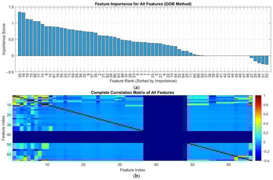
Figure 1.
(a): feature importance ranking using OOB method; (b): feature correlation matrix.
Figure 1a reveals that approximately 66 features significantly influence the algorithm’s predictive performance for mineral scale yield. All but five features showed positive importance scores. These five exceptions with negative scores represent inhibitory factors in mineral scale, likely resulting from their limited representation in the training data. The presence of these negatively scored features, despite their limited data samples, provides critical insights into sedimentation constraints that should be carefully considered in the predictive modeling framework.
Figure 1b presents the complete correlation matrix for all 66 features used in the model, visualized using a color-coded heatmap. The correlation values range from −1 to 1, where light blue and green regions dominate, indicating minimal correlation between most feature pairs. This low linear dependence is advantageous for modeling as it reduces multicollinearity issues. Features 1–11 and 62 represent mineral ions, while the remaining features relate to mineral sedimentation inhibitors. The strongest correlations occur among mineral ion features, reflecting their inherent physical/chemical interdependencies. These ions (e.g., Na+, Cl−, Ca2+, SO42−) directly participate in the chemical processes of inhibitor-containing solutions. Notably, all experimental datasets used for model training consistently reported these ion concentrations, underscoring their fundamental importance. Removing these features could compromise both the model’s generalizability and scientific interpretability, as they represent essential physicochemical parameters in sedimentation phenomena.
Figure 2 presents the prediction results of the GBM algorithm for mineral scale inhibitor efficiency. The model achieved an R2 value of 0.7062, indicating moderate predictive capability. This performance level likely stems from GBM’s ability to handle complex, non-linear relationships between inhibitor dosage and scaling ions. However, the relatively lower R2 compared to other algorithms suggests limitations in capturing subtle interactions between certain ion pairs, particularly at extreme temperature ranges (above 90 °C) where inhibitor performance becomes highly non-linear.
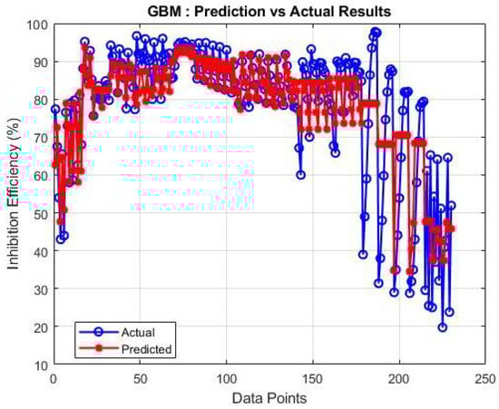
Figure 2.
GBM algorithm performance for mineral scale inhibitor efficiency prediction.
In Figure 3, the performance of the KNN algorithm using the collected database is shown. In Figure 3, the KNN algorithm demonstrates improved performance with an R2 of 0.7731. The better accuracy can be attributed to KNN’s local approximation approach. The remaining prediction errors may occur in samples with unique ion combinations that lack close neighbors in the training set, highlighting a fundamental limitation of distance-based methods in high-dimensional spaces (66 features in this case).
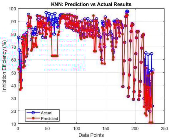
Figure 3.
KNN algorithm evaluation using experimental dataset.
The decision tree algorithm’s performance and quality were also examined to evaluate mineral scale inhibitor efficiency under various ionic and temperature conditions. The decision tree algorithm, shown in Figure 4, achieved a strong R2 of 0.8605. This performance reflects the algorithm’s ability to identify critical thresholds in the data, particularly the important interactions between calcium concentration and temperature (>70 °C) that dominate scaling behavior. The slight underestimation of inhibitor efficiency at high dosage levels suggests the tree depth might have been limited to prevent overfitting.
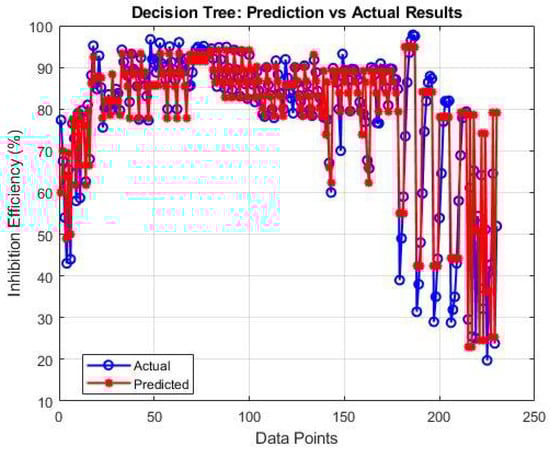
Figure 4.
Decision tree analysis of temperature and ion effects on inhibitors.
Figure 5 displays the superior performance of the random forest algorithm (R2 = 0.8822). The ensemble approach successfully reduces variance compared to a single decision tree, particularly in handling the diverse range of water chemistries present in the dataset. The remaining errors appear clustered around samples with unusually high sulfate concentrations, indicating these cases may require specialized modeling attention.
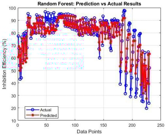
Figure 5.
Random forest model performance for scale inhibition prediction.
Linear regression, as one of the fundamental machine learning regression methods, was used to predict mineral scale inhibitor efficiency in oilfield systems. As shown in Figure 6, linear regression achieved a surprisingly high R2 of 0.8981. This strong performance suggests that many inhibitor–ion interactions follow approximately linear trends within the concentration ranges studied.
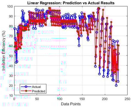
Figure 6.
Linear regression model for inhibitor efficiency estimation.
Given the special importance and wide application of neural networks in chemical systems, this study also employed this method to evaluate mineral scale inhibitor performance in the presence of formation/injection water ions and various inhibitor dosages. The results are presented in Figure 7. The neural network results in Figure 7 show the best performance so far (R2 = 0.9230). The network’s ability to model complex, higher-order interactions between multiple ions and temperature accounts for this improvement.
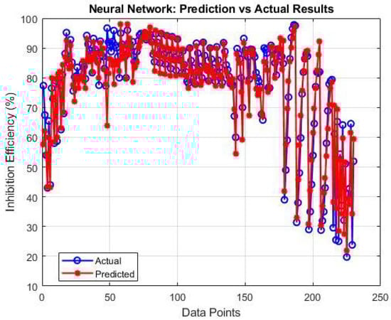
Figure 7.
Neural network evaluation of inhibitor performance.
Figure 8 illustrates the GPR algorithm’s performance compared to actual results using the study’s database of 661 samples and 66 features. Figure 8 demonstrates the exceptional performance of Gaussian process regression (R2 = 0.9608). The GPR’s ability to model uncertainty and capture subtle, non-parametric patterns in the data makes it particularly suited to this application.
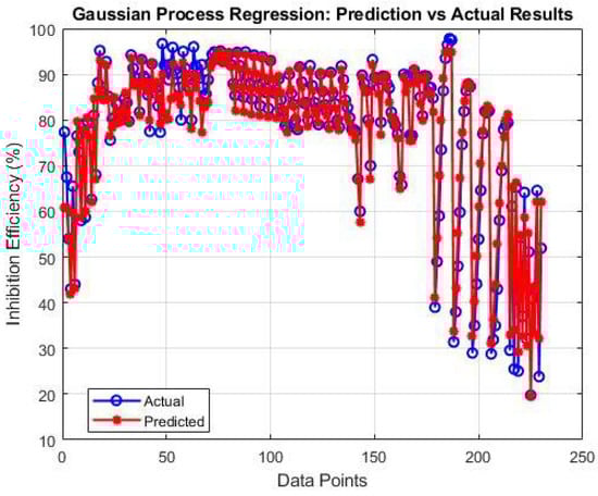
Figure 8.
GPR algorithm performance with experimental validation.
The evaluation of seven machine learning models revealed important insights for predicting mineral scale inhibitor efficiency. When maximum precision is required, Gaussian Process Regression (GPR) emerged as the top performer, achieving excellent accuracy (R2 = 0.96) while providing valuable uncertainty estimates, though it requires more computing power. Neural networks delivered similar accuracy but needed more intensive tuning. For practical field applications that balance speed and accuracy, Linear Regression performed remarkably well with fast processing times, while Random Forest offered dependable predictions with reasonable complexity. These findings highlight that choosing the right model depends on specific operational needs—whether prioritizing precision, speed, or ease of implementation—as each algorithm brings unique strengths to scale inhibitor performance prediction.
The results from testing seven algorithms (Figure 2, Figure 3, Figure 4, Figure 5, Figure 6, Figure 7 and Figure 8) show the following:
- ▪
- Complex models (GPR/Neural Networks) perform best when data is abundant and high accuracy is required;
- ▪
- Simpler models (Linear Regression/Random Forest) are more suitable for routine monitoring;
- ▪
- The optimal model choice depends on specific operational requirements.
4. Conclusions
Produced water in oil reservoirs is a critical fluid that requires regular analysis and evaluation. The presence of mineral ions (such as barium, sodium, calcium, and strontium cations, along with chloride, sulfate, bicarbonate, and carbonate anions) can lead to solution supersaturation and the formation of mineral scales (including barium sulfate, strontium sulfate, calcium sulfate, and calcium carbonate) during water injection operations when incompatible waters mix. One effective method for controlling scale formation is the application of scale inhibitors. This study provides a comprehensive evaluation of scale inhibitor efficiency in oilfield-produced water through advanced machine learning approaches, based on 661 field samples. Among the various algorithms tested, Gaussian Process Regression (GPR) demonstrated the highest prediction accuracy (R2 = 0.9608), making it the most effective model for capturing the complex relationships between chemical concentration and inhibition efficiency. This superior performance is largely attributed to the use of the RBF (Squared Exponential) kernel, which is well suited to the nature of the dataset. Scale inhibition data typically exhibits nonlinear but smooth patterns, as the efficiency of inhibitors like DTPMP, PBTC, EDTMP, ATMP, and HDTMP increases in a predictable yet non-linear fashion with concentration. The RBF kernel assumes smooth functional relationships and allows for interpretable hyperparameters such as length scale and sigma, which control function smoothness and noise level, respectively. By testing a wide range of these parameters using logarithmic spacing, we efficiently explored the parameter space, captured power-law effects inherent in the system, and achieved optimized performance. Other machine learning models such as Neural Network (R2 = 0.9230), Random Forest (R2 = 0.8822), and Decision Tree (R2 = 0.8605) also yielded strong results, while Linear Regression (R2 = 0.8981) performed surprisingly well given its simplicity. However, models like GBM (R2 = 0.7062) and KNN (R2 = 0.7731) were less accurate in capturing the subtle nonlinearities in the data. Overall, these findings underscore the effectiveness of GPR, particularly when combined with appropriate kernel design and parameter optimization, in guiding the selection and optimization of scale inhibitors in oilfield operations.
Supplementary Materials
The following supporting information can be downloaded at: https://www.mdpi.com/article/10.3390/pr13071964/s1, Table S1: Input features and target variable data.
Author Contributions
Conceptualization, S.H.H. and F.T.; methodology, S.H.H. and F.T.; software, S.H.H. and F.T.; validation, S.H.H. and F.T.; formal analysis, S.H.H. and F.T.; writing—original draft preparation, S.H.H. and F.T.; writing—review and editing, F.T.; supervision, F.T. All authors have read and agreed to the published version of the manuscript.
Funding
This research received no external funding.
Data Availability Statement
The original contributions presented in this study are included in the article/supplementary material. Further inquiries can be directed to the corresponding author.
Conflicts of Interest
The authors declare no conflicts of interest.
References
- Hashemi, S.H.; Hashemi, S.A. Prediction of Scale formation according to water injection operations in Nosrat Oil Field. Model. Earth Syst. Environ. 2020, 6, 585–589. [Google Scholar] [CrossRef]
- Hashemi, S.H.; Torghabeh, A.K.; Niknam, A.; Hashemi, S.A.; Gharaie, M.H.M.; Pimentel, N. Geochemical and Thermodynamic Study of Formation Water for Reservoir Management in Bibi Hakimeh Oil and Gas Field, Iran. Fuels 2025, 6, 11. [Google Scholar] [CrossRef]
- Hashemi, S.H.; Besharati, Z.; Torabi, F.; Pimentel, N. Thermodynamic Prediction of Scale Formation in Oil Fields During Water Injection: Application of SPsim Program Through Utilizing Advanced Visual Basic Excel Tool. Processes 2024, 12, 2722. [Google Scholar] [CrossRef]
- Haghtalab, A.; Kamali, J.; Shahrabadi, A. Prediction mineral scale formation in oil reservoirs during water injection. Fluid Phase Equilibria 2014, 373, 43–54. [Google Scholar] [CrossRef]
- Shabani, A.; Sisakhti, H.; Sheikhi, S.; Barzega, F. A reactive transport approach for modeling scale formation and deposition in water injection wells. J. Pet. Sci. Eng. 2020, 190, 107031. [Google Scholar] [CrossRef]
- Ardakani, S.F.G.; Hosseini, S.T.; Kazemzadeh, Y. A review of scale inhibitor methods during modified smart water injection. Can. J. Chem. Eng. 2024, 102, 3922. [Google Scholar] [CrossRef]
- Mpelwa, M.; Tang, S.F. State of the art of synthetic threshold scale inhibitors for mineral scaling in the petroleum industry: A review. Pet. Sci. 2019, 16, 830–849. [Google Scholar] [CrossRef]
- Housse, M.E.; Hadfi, A.; Iberache, N.; Karmal, I.; El-Ghazouani, F.; Ben-aazza, S.; Belattar, M.; Ammayen, I.; Nassiri, M.; Darbal, S.; et al. Eco-friendly and sustainable approaches to control scaling in industrial plants: Challenges and advantages of the application of plant extracts as a probable alternative for traditional inhibitor-A review. Ind. Crops Prod. 2024, 222, 120030. [Google Scholar] [CrossRef]
- Chaussemier, M.; Pourmohtasham, E.; Gelus, D.; Pécoul, N.; Perrot, H.; Lédion, J.; Cheap-Charpentier, H.; Horner, O. State of art of natural inhibitors of calcium carbonate scaling. A review article. Desalination 2015, 356, 47–55. [Google Scholar] [CrossRef]
- Husna, U.Z.; Elraies, K.A.; Shuhili, J.A.B.M.; Elryes, A.A. A review: The utilization potency of biopolymer as an eco-friendly scale inhibitors. J. Pet. Explor. Prod. Technol. 2022, 12, 1075–1094. [Google Scholar] [CrossRef]
- Freitas, V.M.S.; Paschoalino, W.J.; Vieira, L.C.S.; Silva, J.M.; Couto, B.C.; Gobbi, A.L.; Lima, R.S. Sensitive Monitoring of the Minimum Inhibitor Concentration under Real Inorganic Scaling Scenarios. ACS Omega 2024, 9, 39724–39732. [Google Scholar] [CrossRef] [PubMed]
- Yang, J.; Jia, L.; Wang, Z.; Niu, C.; Zhou, H.; Wang, Z.; Li, Y.; Chen, Y. Synthesis and scale inhibition performance of a novel phosphorus-free scale inhibitor–polyethylenebismaleamic acid-ethylenediamine. J. Mol. Struct. 2025, 1335, 141950. [Google Scholar] [CrossRef]
- Hu, H.; Wang, J.-J.; Ma, W.; Li, G.; Wang, L.-C. Effect of the ratio of carboxyl group to ethylene oxide on performance of acrylic acid based copolymer scale inhibitors. Desalination Water Treat. 2025, 321, 101035. [Google Scholar] [CrossRef]
- Zhang, P.; Zhang, Z.; Liu, Y.; Kan, A.; Tomson, M. Investigation of the impact of ferrous species on the performance of common oilfield scale inhibitors for mineral scale control. J. Pet. Sci. Eng. 2019, 172, 288–296. [Google Scholar] [CrossRef]
- Khormali, A.; Bahlake, G.; Struchkov, I.; Kazemzadeh, Y. Increasing inhibition performance of simultaneous precipitation of calcium and strontium sulfate scales using a new inhibitor—Laboratory and field application. J. Pet. Sci. Eng. 2021, 202, 10. [Google Scholar] [CrossRef]
- Khormali, A.; Sharifov, A.; Torba, D. Increasing efficiency of calcium sulfate scale prevention using a new mixture of phosphonate scale inhibitors during waterflooding. J. Pet. Sci. Eng. 2018, 164, 245–258. [Google Scholar] [CrossRef]
- Zakaria, K.; Salem, A.; Ramzi, M. Cost-effective and eco-friendly organophosphorus-based inhibitors for mineral scaling in Egyptian oil reservoirs: Theoretical, experimental and quantum chemical studies. J. Pet. Sci. Eng. 2020, 195, 107519. [Google Scholar] [CrossRef]
- Khodabakhshi, M.; Bijani, M. Predicting Scale Deposition in Oil Reservoirs Using Machine Learning Optimization Algorithms. Results Eng. 2024, 22, 102263. [Google Scholar] [CrossRef]
- Handhal, A.; Al-Abadi, A.; Chafeet, H.; Ismail, M. Prediction of total organic carbon at Rumaila oil field, Southern Iraq using conventional well logs and machine learning algorithms. Mar. Pet. Geol. 2020, 116, 104347. [Google Scholar] [CrossRef]
- Zaiery, M.; Kadkhodaie, A.; Arian, M.; Maleki, Z. Application of artificial neural network models and random forest algorithm for estimation of fracture intensity from petrophysical data. J. Pet. Explor. Prod. Technol. 2023, 13, 1877–1887. [Google Scholar] [CrossRef]
- Al-Mudhafar, W.J. Integrating well log interpretations for lithofacies classification and permeability modeling through advanced machine learning algorithms. J. Pet. Explor. Prod. Technol. 2017, 7, 1023–1033. [Google Scholar] [CrossRef]
- Mahdaviara, M.; Rostami, A.; Keivanimehr, F.; Shahbazi, K. Accurate determination of permeability in carbonate reservoirs using Gaussian Process Regression. J. Pet. Sci. Eng. 2020, 196, 107807. [Google Scholar] [CrossRef]
- Khormali, A.; Petrakov, D.G.; Nazari Moghaddam, R. Study of adsorption/desorption properties of a new scale inhibitor package to prevent calcium carbonate formation during water injection in oil reservoirs. J. Pet. Sci. Eng. 2017, 153, 257–267. [Google Scholar] [CrossRef]
- Khormali, A.; Petrakov, D.G.; Moein, M. Experimental analysis of calcium carbonate scale formation and inhibition in waterflooding of carbonate reservoirs. J. Pet. Sci. Eng. 2016, 147, 843–850. [Google Scholar] [CrossRef]
- Khormali, A.; Sharifov, A.R.; Torba, D.I. Investigation of Barium Sulfate Precipitation and Prevention Using Different Scale Inhibitors under Reservoir Conditions. Int. J. Eng. 2018, 31, 1796–1802. [Google Scholar]
- Khormali, A.; Petrakov, D.G.; Shcherbakov, G.Y. An In-depth Study of Calcium Carbonate Scale Formation and Inhibition. Iran. J. Oil Gas Sci. Technol. 2014, 3, 67–77. [Google Scholar]
- Khormali, A.; Petrakov, D.G.; Lamidi, A.-L.B.; Rastegar, R. Prevention of Calcium Carbonate Precipitation during Water Injection into High-Pressure High-Temperature Wells. In Proceedings of the SPE European Formation Damage Conference and Exhibition, Budapest, Hungary, 3–5 June 2015. [Google Scholar]
- Li, G.; Guo, S.; Zhang, J.; Liu, Y. Inhibition of scale buildup during produced-water reuse: Optimization of inhibitors and application in the field. Desalination 2014, 351, 213–219. [Google Scholar] [CrossRef]
- Azizi, J.; Shadizadeh, S.R.; Manshad, A.; Mohammadi, A. A dynamic method for experimental assessment of scale inhibitor efficiency in oil recovery process by water flooding. Petroleum 2019, 5, 303–314. [Google Scholar] [CrossRef]
- Hastie, T.; Tibshirani, R.; Friedman, J. The Elements of Statistical Learning: Data Mining, Inference, and Prediction, 2nd ed.; Springer: New York, NY, USA, 2009. [Google Scholar]
- Cao, C. Prediction of concrete porosity using machine learning. Results Eng. 2023, 17, 100794. [Google Scholar] [CrossRef]
- Attanasi, E.D.; Coburn, T.C. Random Forest. In Encyclopedia of Mathematical Geosciences; Daya Sagar, B.S., Cheng, Q., McKinley, J., Agterberg, F., Eds.; Encyclopedia of Earth Sciences Series; Springer: Cham, Switzerland, 2023. [Google Scholar]
- Breiman, L. Random forests. Mach. Learn. 2001, 45, 5–32. [Google Scholar] [CrossRef]
Disclaimer/Publisher’s Note: The statements, opinions and data contained in all publications are solely those of the individual author(s) and contributor(s) and not of MDPI and/or the editor(s). MDPI and/or the editor(s) disclaim responsibility for any injury to people or property resulting from any ideas, methods, instructions or products referred to in the content. |
© 2025 by the authors. Licensee MDPI, Basel, Switzerland. This article is an open access article distributed under the terms and conditions of the Creative Commons Attribution (CC BY) license (https://creativecommons.org/licenses/by/4.0/).