Abstract
Long-term shutdowns caused by ice formation on wind turbine blades can lead to significant power generation losses, a persistent issue for wind farm operators. The rapid acquisition of ice mass and thickness on blades under actual meteorological conditions can facilitate the more effective adjustment of operation and maintenance strategies, enabling the selection of appropriate de-icing methods and optimal human resource allocation. This study proposes a novel approach utilizing icing simulation data across various meteorological parameters to train a Multilayer Perceptron (MLP) neural network, enabling rapid ice accretion prediction while maintaining acceptable accuracy. The results demonstrate that the MLP model achieves mean absolute percentage errors (MAPEs) of 7.13% and 7.02% for predicting rime ice mass and maximum thickness, respectively. For glaze ice prediction, the model yields MAPE values of 10.22% and 9.42% for ice mass and maximum thickness prediction, respectively. All MLP models exhibit R2 values exceeding 0.95, indicating excellent model fitting. The model is used to simulate and analyze the blade icing condition of a wind farm (located at 27° N and 117° E). The results showed that during a typical icing cycle, the maximum hourly ice accumulation mass on the studied blade was 5.01 kg, and the accumulated ice accumulation mass over 24 h was 95.43 kg. The maximum hourly ice accumulation thickness was 10.38 mm, and the accumulated ice accumulation thickness over 24 h was 228.43 mm.
1. Introduction
High-altitude areas typically boast higher wind speeds, enhancing the power generation potential of wind farms [1]. However, these regions also face colder temperatures, leading to ice formation on wind turbine blades [2]. With the increasing construction of wind farms, the icing problem is receiving more attention. Ice accumulation can cause a decrease in power generation [3], an impact on the mechanical structure of the turbine [4], a reduction in the aerodynamic characteristics [5], safety risks to the wind farm [6], and wind energy losses [7]. According to relevant reports, the annual loss of wind power caused by ice accretion is as high as 17% [8]. Usually, when the blades are frozen, the wind farm triggers an alarm to prevent damage to the blades, causing the wind turbine to stop [4]. The lack of monitoring systems results in wind turbines not operating even when the start-up conditions are met, which wastes many wind resources [9]. Wind farms need appropriate start-up time to reduce wind energy waste [10]. The icing condition of the blades, a critical criterion for determining the operational readiness of wind turbines, becomes particularly challenging to assess in high-altitude mountainous areas. These environments are often shrouded in thick fog and persistent cloud cover [11], complicating visual inspections of blade icing. Therefore, practical methods for predicting ice conditions on blade surfaces urgently need to be designed. Effective icing process prediction methods can provide the necessary decision support for the operation of wind farms, such as adjusting start–stop strategies or implementing anti-icing/de-icing measures to reduce risks and efficiency losses caused by ice.
Forecasting is typically based on meteorological data, icing models, and data analysis of historical icing events [12]. In their research on prediction methods for icing conditions, Bose et al. [13] experimentally studied the ice profiles of small horizontal-axis wind turbine blades at different wingspan positions. Fu et al. [14] simulated the process of rime ice accumulation on a horizontal-axis wind turbine operating under icing conditions. Han et al. [15] introduced the icing test of a blade installed on a rotor test bench and obtained some test procedures and experimental data. Wang et al. [16] proposed an improved icing calculation model to simulate the icing situation of wind turbines under yaw conditions. Chuang et al. [17,18] found that the blade ice absorption increased linearly along the blade span, mainly concentrated at the blade’s leading edge. Ibrahim et al. [19,20] proposed a dimensionless model for the flow field and droplet trajectory of glaze and rime ice on rotating wind turbine blades, and they conducted a numerical CFD icing simulation using ANSYS FENSAP-ICE software (version:22.1, ANSYS Inc., Canonsburg, PA, USA). Cao et al. [21] used a combination of FLUENT and FENSAP-ICE software to analyze the icing sensitivity of offshore wind turbine blades. They also analyzed the effects of the liquid water content (LWC), median volume diameter (MVD), wind speed, and temperature on the shape of blade icing. Shu et al. [22] conducted experimental research on the icing characteristics and output of small horizontal-axis wind turbines in an artificial climate chamber. They proposed a three-dimensional icing wind turbine model to simulate glazed ice. In summary, there have been some experimental and simulation studies that can predict the growth position and shape of the ice accretion on the blade’s surface. However, the dynamic icing of large wind turbine blades is a rather complex problem, limited by the influence of climatic conditions and the difficulty of obtaining actual data on site.
Numerical simulation is no longer limited by on-site conditions when solving the simulation problem of large-scale blade ice accretion. It can accurately provide detailed physical information related to aerodynamics and thermodynamics. However, numerical simulation requires a large amount of computation and time, which poses difficulties for processing large-scale data and real-time prediction. Unlike traditional machine learning, neural networks and reinforcement learning models can effectively handle complex pattern recognition, nonlinear mapping, and large-scale data analysis. Combining these advantages can achieve more efficient and accurate ice layer simulation and prediction. By combining CFD and neural network methods, new ideas and approaches can be provided to improve the effectiveness of blade icing simulation and prediction. Researchers use the artificial neural network (ANN) in some fields to estimate wind turbine icing. Li et al. [23] designed a general model based on deep neural networks (DNNs) which uses data from monitoring and data acquisition systems. The authors transferred some feature variables related to wind turbine blade icing from previous research to obtain a model that can accurately predict whether the wind turbine is icing. Kreutz et al. [24] applied a dual-input, one-dimensional convolutional neural network to predict 24 h icing risks using historical wind turbine data and weather forecasts, achieving a 97.9% average balanced accuracy across three wind farms. Ye et al. [10] designed a machine learning framework to capture unique icing event features. These, along with power curve features, trained a deep learning model to accurately classify and quantify icing probabilities. Although neural networks have made some progress in the field of icing prediction, most of them are used for early warning about wind turbine icing. More research is still needed on combining neural network methods with data to predict icing.
This work is essentially about the build-up of ice on wind farm rotor blades based on the prevalent weather conditions. This work uses what is now a standard technique in many areas using neural networks and develops a training, validation, and test procedure. The idea is that the data already available remotely on wind speed, humidity, and temperature, etc., can be used to show the build-up of ice. The aim of this work is to help wind farms save a lot of time and enable timely de-icing, restoring the rotor/turbine to its optimal performance.
2. Implementation of CFD Simulation
2.1. Blade Element
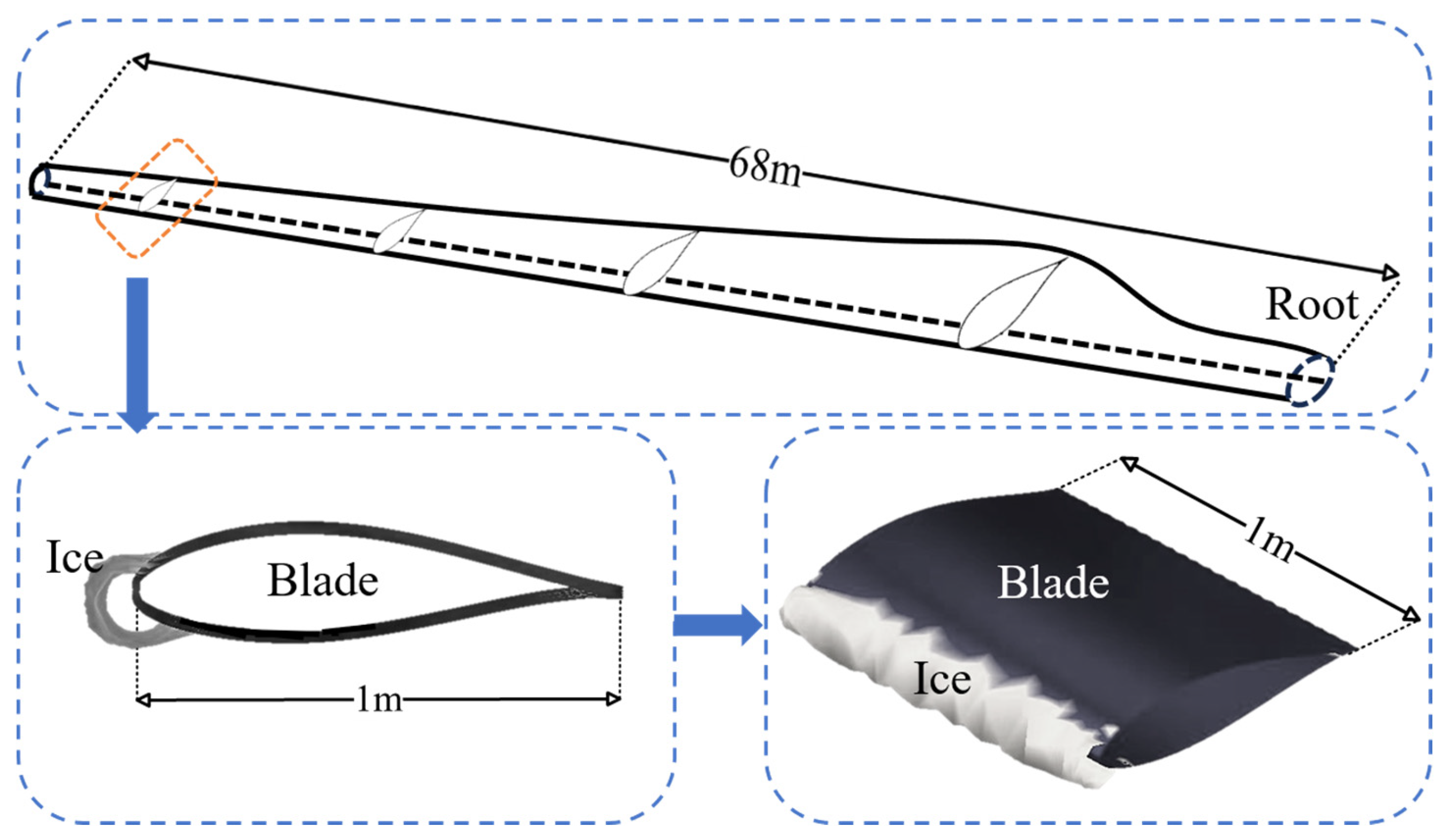
Icing data obtained through CFD numerical simulations under diverse meteorological conditions were used to train the MLP model. The blade model used in this study is NACA4421, with a total length (L) of 68 m. Since maintenance personnel typically prioritize sections with severe icing, this study focuses on a blade element exhibiting significant ice accumulation for detailed analysis. Previous studies have demonstrated that ice accumulation on the blade increases linearly from the root to approximately half of its length (1/2 L). In contrast, the ice thickness remains relatively constant from 1/2 L to the tip [25], with the most severe icing occurring between ½ L and the tip. Therefore, the optimal position for the selected blade component in this study is within the range of 1/2 L to the blade tip.
In previous studies, blade elements with a length of 1 m were commonly selected. For the blade under investigation, a 1 m blade element located 60 m from the root falls within the range of 1/2 L from the blade tip. To meet operational and maintenance requirements while facilitating data comparison and verification related to ice accumulation, a blade element with a radial length of 1 m and positioned 60 m from the blade root was chosen for analysis. As shown in Figure 1, a three-dimensional model with a radial span of 1 m was developed to accurately simulate and measure ice accretion.
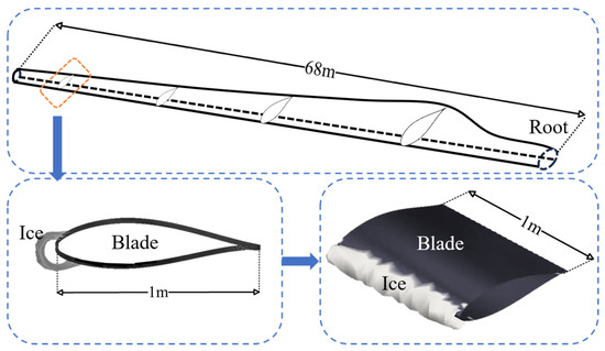
Figure 1.
Location and size diagram of the studied blade element.
2.2. Meteorological Conditions and Icing State Parameters
In numerical simulations for ice accretion calculation, selecting key climatic parameters as variables is critical. As demonstrated in previous studies [26,27,28,29,30], the temperature, inflow velocity, LWC, blade angle of attack, and MVD significantly influence the ice accretion process. When the temperature falls below the freezing point, liquid water freezes, and the temperature affects the ice structure. An appropriate increase in inflow velocity results in more water droplets impinging on the surface, accelerating the icing rate. Higher LWC values correspond to greater amounts of freezable water. Variations in the angle of attack alter the airflow patterns around the blades, consequently affecting the impact position and coverage area of water droplets. Larger MVD values indicate that water droplets possess greater kinetic energy, making them more likely to impact the surface.
While the MVD significantly influences ice accretion, its variability is relatively limited within specific geographic regions. Compared to other factors, the angle of attack exhibits a comparatively minor effect. Therefore, this study focuses on the inflow velocity, temperature, and LWC as the primary computational variables for simulation. Specifically, temperature refers to the ambient temperature surrounding the blades (°C), the LWC denotes the liquid water content in the blade environment (g/m3), and the inflow velocity represents the resultant velocity combining blade rotational speed and natural wind speed (m/s).
Due to the diverse ice types formed under varying climatic conditions, distinct modeling approaches are required for accurate numerical simulations of icing scenarios. Ice accretion on blades can be classified into three categories based on environmental temperature: glaze ice, rime ice, and mixed ice. Glaze ice typically forms between −10 °C and 0 °C when supercooled water droplets impact the surface and rapidly freeze [31]. Rime ice primarily forms at temperatures significantly below −10 °C. When humid air comes into contact with a cooled surface, water vapor directly condenses into rime ice, which is characterized by a white, rough surface and a loose, porous structure. Rime ice forms rapidly and can cover extensive areas in a short period. Mixed ice forms in environments with frequent fluctuations in temperature and humidity, particularly when temperatures oscillate around −10 °C, exhibiting characteristics of both glaze and rime ice simultaneously [15,32].
In this study, the primary focus is on glaze ice and rime ice. Specifically, ice formed between −10 °C and 0 °C is classified as glaze ice, and the glaze ice model is employed for calculations. Conversely, ice formed below −10 °C is classified as rime ice, and the rime ice model is utilized for calculations.
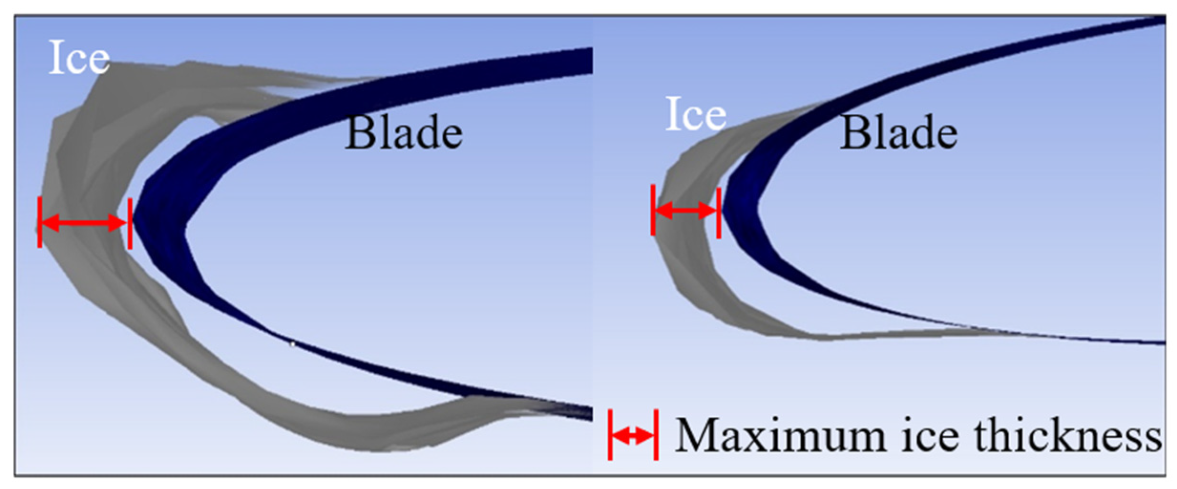
Two metrics are employed to quantify the icing conditions: the ice accretion mass and maximum ice thickness. The ice accretion mass is defined as the mass of ice accumulated on a 1 m chord length section of a blade at a 1 m radial length, measured in kilograms. In this study, regardless of the ice type, the maximum ice thickness refers to the greatest transverse distance of ice accumulation from the leading edge of a blade element to the tip of the ice at that leading edge, as shown in Figure 2, measured in millimeters.

Figure 2.
Sketch map of maximum ice thickness.
2.3. Assumptions
The actual process of blade icing is highly complex, and certain simplifications are necessary to facilitate numerical simulations. Therefore, the following assumptions are proposed:
- (1)
- Three-dimensional and rotational effects on the icing process are neglected;
- (2)
- The icing process is studied based on blade elements, with no interaction between adjacent blade elements;
- (3)
- Water droplets are uniformly distributed in the air;
- (4)
- The blade surface is adiabatic.
2.4. Simulation Software and Basic Parameters
This study first utilized FLUENT software to calculate the flow field around the blade. The simulation results of the flow field were then imported into the FENSAP-ICE module in ANSYS to compute the water droplet collision coefficient and simulate blade icing. The trajectory of water droplets was simulated by solving the droplet motion equations that interact with the flow field. The calculation of water droplet trajectories is based on the Eulerian two-fluid model. FENSAP-ICE determined the impact positions and velocities of water droplets on the blade surface. Subsequently, the collection efficiency of water droplets on the blade surface under specific operating conditions was evaluated. The Shallow-Water Icing Model was used to solve the water film flow, applying Newton’s shear law to model the water film flow. This model neglects the effects of gravity and surface tension and adopts the average temperature assumption, implying no temperature gradient along the thickness direction of the water film.
In this study, the water droplet diameter was 20 μm, and the freezing duration was 3600 s. Consequently, ice mass and maximum ice thickness values were obtained for various operating conditions. The computational domain and grid used in this study are shown in Figure 3.
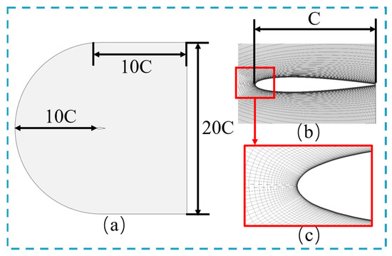
Figure 3.
Computational domains: (a) monolithic domain; (b) blade; and (c) leading edge of blade.
2.5. Simulation Verification
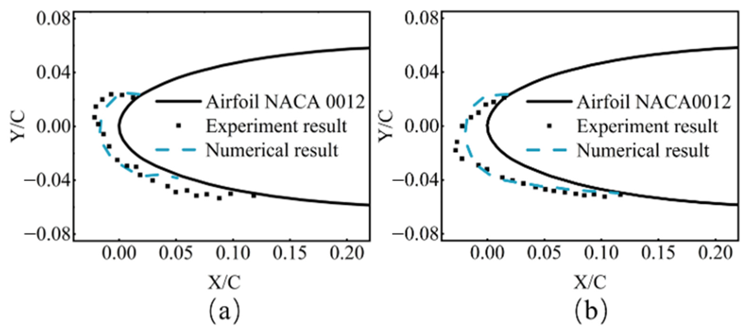
Simulation conditions: the airfoil is NACA0012; the chord length is 0.5334 m; the pressure is 101,300 Pa; the free flowing velocity is 102 m/s; the LWC is 0.55 g/m3; the MVD is 20 μm; the accumulation time is 480 s; the angle of attack is 4°; and the temperature is −6 °C for glaze ice and −26 °C for rime ice.
As shown in Figure 4, compared with the data obtained in the laboratory under the same operating conditions [27], the maximum thickness of glaze ice and rime ice is basically the same. Notably, the maximum thickness defined in this study is the greatest transverse distance of ice accumulation from the leading edge of a blade element to the tip of the ice at that leading edge. By observing the area of ice, the results of the rime ice were determined to be better, and both glaze ice and rime ice can meet engineering requirements. These validations ensure the simulation results’ accuracy and provide a robust foundation for subsequent research on icing prediction and analysis under similar conditions.
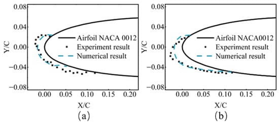
Figure 4.
Simulation verification: (a) glaze ice and (b) rime ice.
3. Implementation of MLP Model
3.1. Neural Network
An ANN is a computational model inspired by the principles of neural connectivity in the human brain [33]. The fundamental building blocks of ANNs are artificial neurons, which are analogous to biological neurons. ANNs consist of interconnected neurons that collectively process complex data relationships [34]. The connections between neurons are associated with different weights, representing the magnitude of influence one neuron has on another. Each neuron performs a specific function: data from other neurons undergo weighted calculations and are then passed through an activation function to produce a new output value [35]. This process enables neural networks to learn complex patterns and functional relationships.
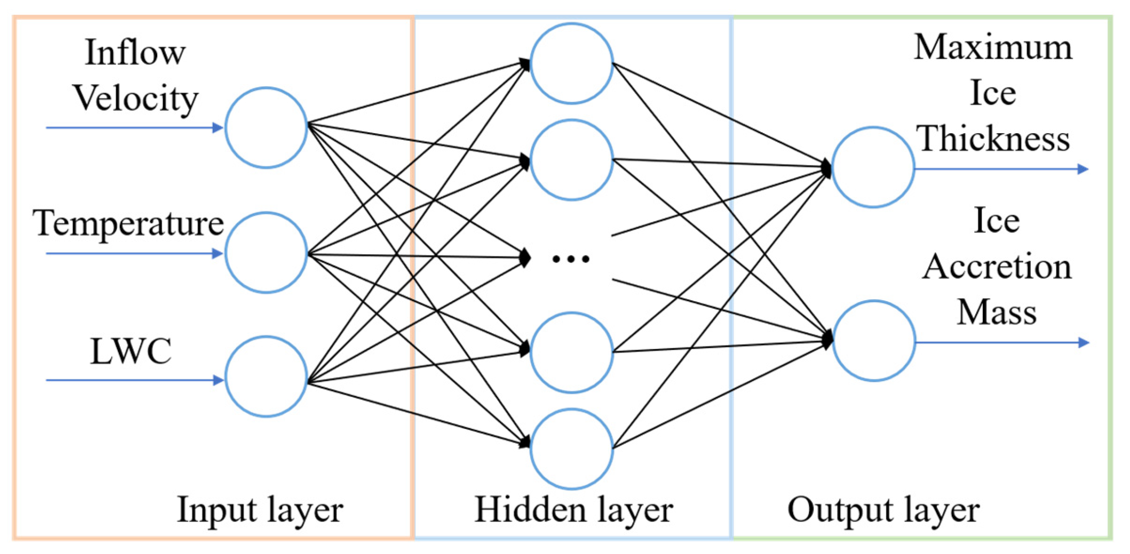
An MLP is a widely used type of feedforward neural network. Its structure comprises an input layer, one or more hidden layers, and an output layer. Information flows in a fully connected way from the input layer to the hidden layer, from the hidden layer to the output layer, and between continuous hidden layers [36]. This structure ensures comprehensive information propagation throughout the network. Notably, neurons within the same layer are not interconnected. Figure 5 illustrates a three-layer MLP neural network structure.
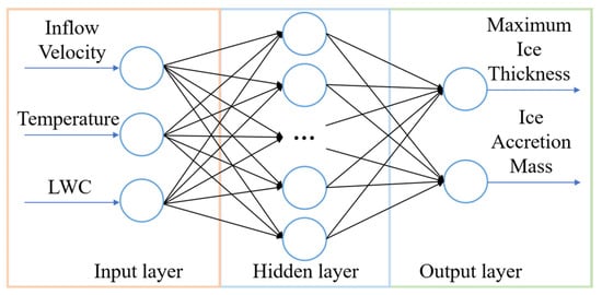
Figure 5.
MLP neural network structure diagram.
The training process for an MLP is typically performed using the backpropagation (BP) algorithm, which propagates errors from the output layer back to the input layer, implementing an error correction mechanism [37]. Based on the errors from the previous iteration, the weights in the neural network model are adjusted through the BP algorithm. This mechanism ensures that the neural network’s output progressively aligns with the CFD simulation results during training.
This study employed an MLP neural network to handle small-sample regression tasks, primarily due to its strong nonlinear fitting capabilities.
3.2. Dataset and Dataset Division
Eighty-one simulation conditions (Table S1) were designed for both glaze and rime ice, as shown in Table 1, and the corresponding ice accretion mass and maximum ice thickness values were extracted from the simulation data for each condition.

Table 1.
Simulation conditions.
For rime ice conditions, an orthogonal table (81.9.3) suitable for studying rime ice formation was selected for the simulation design. Based on its characteristics, 81 operating conditions were designed to investigate the effects of the temperature, liquid water content, and inflow velocity on rime ice formation across different levels. For each of the three factors, nine levels were defined. The temperature levels were set at −11 °C, −12 °C, −13 °C, −14 °C, −15 °C, −16 °C, −17 °C, −18 °C, and −19 °C. The liquid water content levels were set at 0.30 g/m3, 0.45 g/m3, 0.60 g/m3, 0.75 g/m3, 0.90 g/m3, 1.05 g/m3, 1.20 g/m3, 1.35 g/m3, and 1.50 g/m3. The inflow velocities were set at 10 m/s, 20 m/s, 30 m/s, 40 m/s, 50 m/s, 60 m/s, 70 m/s, 80 m/s, and 90 m/s.
Similarly, based on the characteristics of glaze ice, 81 operating conditions were designed. For each of the three factors, nine levels were defined. The temperature levels were set at −2 °C, −3 °C, −4 °C, −5 °C, −6 °C, −7 °C, −8 °C, −9 °C, and −10 °C. The liquid water content levels were set at 1.0 g/m3, 1.5 g/m3, 2.0 g/m3, 2.5 g/m3, 3.0 g/m3, 3.5 g/m3, 4.0 g/m3, 4.5 g/m3, and 5.0 g/m3. The inflow velocities were set at 10 m/s, 20 m/s, 30 m/s, 40 m/s, 50 m/s, 60 m/s, 70 m/s, 80 m/s, and 90 m/s.
Data for the rime ice maximum thickness and accretion mass (81 sets of data each) and data for the glaze ice maximum thickness and accretion mass (81 sets of data each) were trained separately. Among these, 57 data points were allocated to the training set (70%), 12 data points to the validation set (15%), and the remaining 12 data points to the testing set (15%), all of which were randomly divided. The training set was used for initial model training, while the validation set ensured the model’s generalizability by preventing overfitting. Finally, the testing set was employed to evaluate the model’s performance.
3.3. Neural Network Structure Design
The dimensionality of the feature variables in the sample input determines the number of neurons in the input layer. After preparing the blade icing dataset, the inflow velocity, temperature, and LWC are used as inputs. Consequently, the input layer of each MLP contains three neural units.
This study completely separates the tasks of predicting the ice accretion mass and the maximum ice thickness, with each model dedicated to a single output (one for ice accretion mass and the other for maximum ice thickness). This approach allows for the optimization of the network architecture and hyperparameters for each specific task, thereby enhancing individual task performance. Consequently, the output layer of each MLP contains one neuron.
To enhance the predictive capability of the network, nonlinearity is introduced through the activation functions of the hidden layer neurons. Specifically, the Sigmoid function is employed as the activation function for the hidden layer. The Sigmoid function can accept any input value, while its output is constrained to the range [0, 1]. The linear activation function (purelin) is selected for the output layer neuron, as it allows any input and output values, making it suitable for continuous-value targets [38]. The mathematical expressions for these functions are as follows:
where x is the input variable.
Selecting too few neurons in the hidden layer can compromise network performance, while choosing too many may result in prolonged training times, increased susceptibility to local minima, and a higher risk of overfitting. There is no definitive rule for determining the optimal number of hidden layers or neurons; this is typically addressed through an iterative trial-and-error process, comparing the performance of various architectures after training. Given this study’s limited dataset and only three input variables, the complexity remains manageable. Therefore, a single hidden layer is considered appropriate. Previous theoretical studies have derived empirical formulas for determining the number of neurons in single-hidden-layer networks, as follows [39]:
where a is the number of hidden layer neurons, m is the number of input layer neurons, n is the number of output layer neurons, and α is a random constant between 1 and 10.
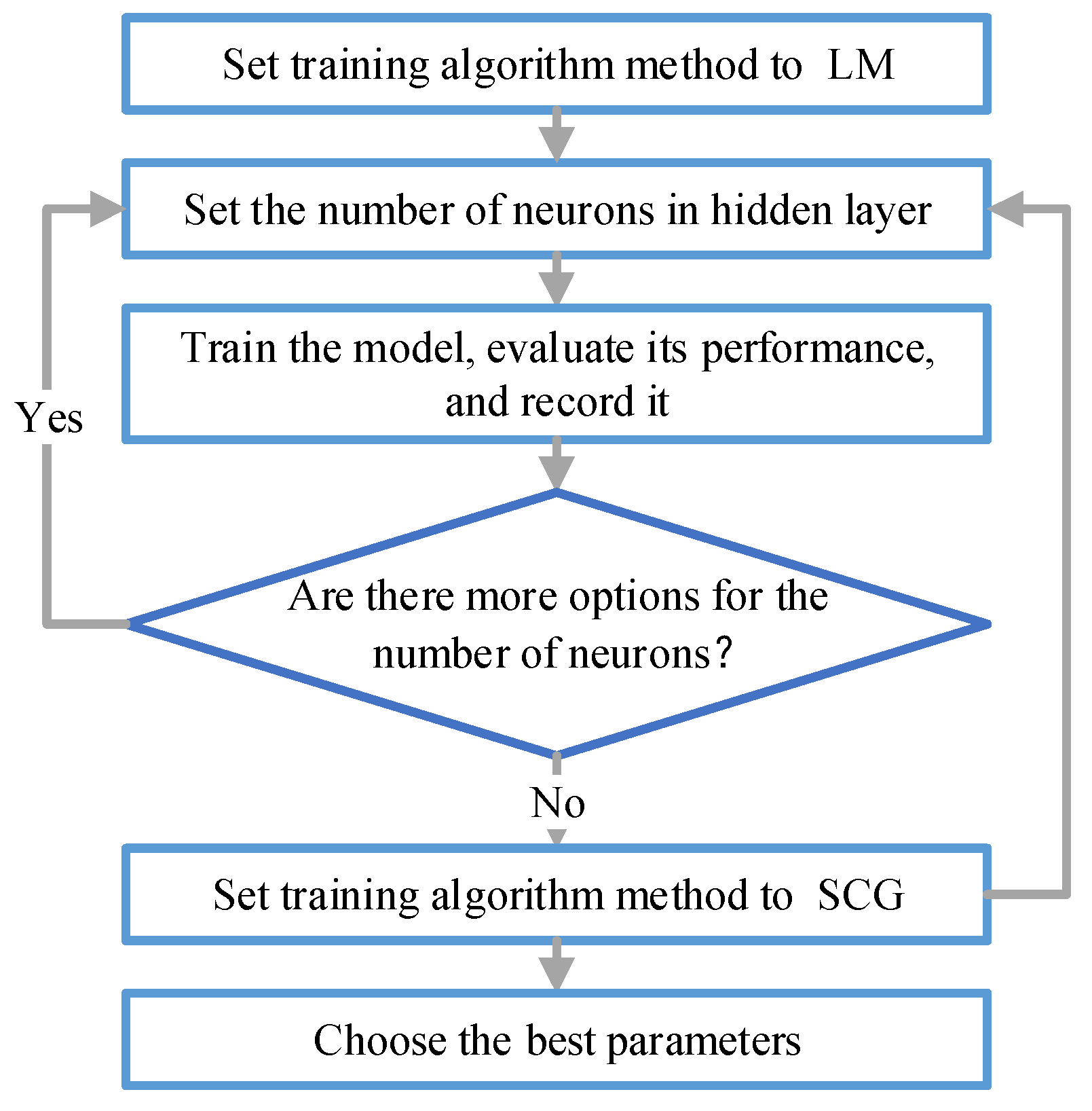
Based on the empirical formula, the number of neurons in the hidden layer is determined to fall within the interval [3,12]. To enhance the reliability of the results, the model’s performance is evaluated across an extended interval of neurons, specifically [1,15], following the methodology illustrated in Figure 6. The performance is assessed using two key metrics: the Mean Squared Error (MSE) and the Pearson correlation coefficient (R). The MSE, also called the L2 norm loss, is a widely utilized measure for quantifying model prediction errors. A lower MSE value, ideally approaching 0, indicates a better fit of the model. The R is a statistical measure that evaluates the strength and direction of the linear relationship between two continuous variables. This parametric statistic ranges from −1 to 1, where values closer to ±1 denote stronger linear relationships, with the sign indicating the direction of covariation (positive or negative). In contrast, an R value of 0 signifies the absence of a linear correlation. In selecting the optimal model configuration, primary emphasis is placed on the MSE and R values. The corresponding formulas are structured as follows:
where is the actual value of the sample, is the mean of the actual value, is the predicted value of the sample, is the mean of the predicted value, and is the total sample size.
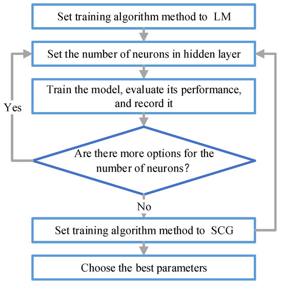
Figure 6.
The flowchart of selecting the optimal MLP.
To achieve optimal predictive performance, two optimization algorithms were implemented following the methodology illustrated in Figure 6. The Levenberg–Marquardt (LM) algorithm, known as damping least squares, was employed to address nonlinear least squares problems [40]. This algorithm is widely recognized as the most frequently used method for optimizing weights and biases in MLP neural networks. Additionally, the Scaled Conjugate Gradient (SCG) algorithm, which operates within a gradient descent framework, was utilized to expedite the optimization process by conducting searches in the conjugate direction. In applying SCG, the search direction was aligned with the steepest descent of the gradient function, ensuring minimal error while maintaining computational efficiency [41].
Additional evaluation metrics, including the coefficient of determination (R2) and the MAPE, were incorporated to facilitate a comprehensive analysis of the MLP’s performance.
The R2, also called the goodness of fit, quantifies the proportion of variability in the dependent variable explained by the independent variables in a regression model. R2 values range from 0 to 1, with higher values indicating a better fit. For example, an R2 value of 0.5 indicates that the independent variables account for 50% of the variability in the dependent variable.
The MAPE is a variant of the mean absolute error expressed as a percentage. Unlike other error metrics, the MAPE is less sensitive to outliers, as it considers the ratio of the absolute error to the actual values. A lower MAPE value signifies a better model fit.
The calculation formulas for each evaluation metric are as follows:
where and are the real and estimated outputs, respectively, is the mean of the actual value, and is the number of data points in each section.
The numerical simulation was performed using an AMD Ryzen 5 3600 6-Core Processor operating at 3.59 GHz, with 16.0 GB of RAM (Santa Clara, CA, USA). The simulations were executed using ANSYS 2022R, while the network training was conducted in MATLAB R2021b. On average, each icing simulation condition required approximately 30 min of computation time.
4. Results and Discussion
4.1. Final Model Configuration
Table 2, Table 3, Table 4 and Table 5 present the results of selecting the number of hidden layer neurons and algorithms. The numbers in parentheses indicate the optimal number of neurons within the given range. To reduce the impact of randomness, the MSE and R values reported in the tables represent the average of 10 training iterations using identical parameters. In determining the number of neurons, it is crucial to consider the performance of the training set, testing set, and validation set comprehensively. As evidenced in Table 2, Table 3, Table 4 and Table 5, certain models demonstrated excellent fitting performance on the training and validation sets but exhibited suboptimal results on the test set. Based on a comprehensive evaluation, the final model configurations were determined as follows: two neurons for rime ice accretion mass prediction, five neurons for maximum rime ice accretion thickness prediction, three neurons for glaze ice mass prediction, and four neurons for maximum glaze ice accretion thickness prediction.
Table 2.
Some MLP architectures used for ice accretion mass in rime ice prediction.
Table 3.
Some MLP architectures used for maximum ice thickness in rime ice prediction.
Table 4.
Some MLP architectures used for ice accretion mass in glaze ice prediction.
Table 5.
Some MLP architectures used for maximum ice thickness in glaze ice prediction.
4.2. Model Performance Evaluation
After determining the optimal parameters for the neural networks, four MLP models were developed to estimate the mass and maximum thickness of rime ice and glaze ice accretion. Each model was trained ten times, and the network with the best predictive performance was selected for further analysis. This section presents and discusses the key results of the performance evaluation. A comprehensive assessment and comparison of each model’s performance during network training were conducted to ensure reliability.
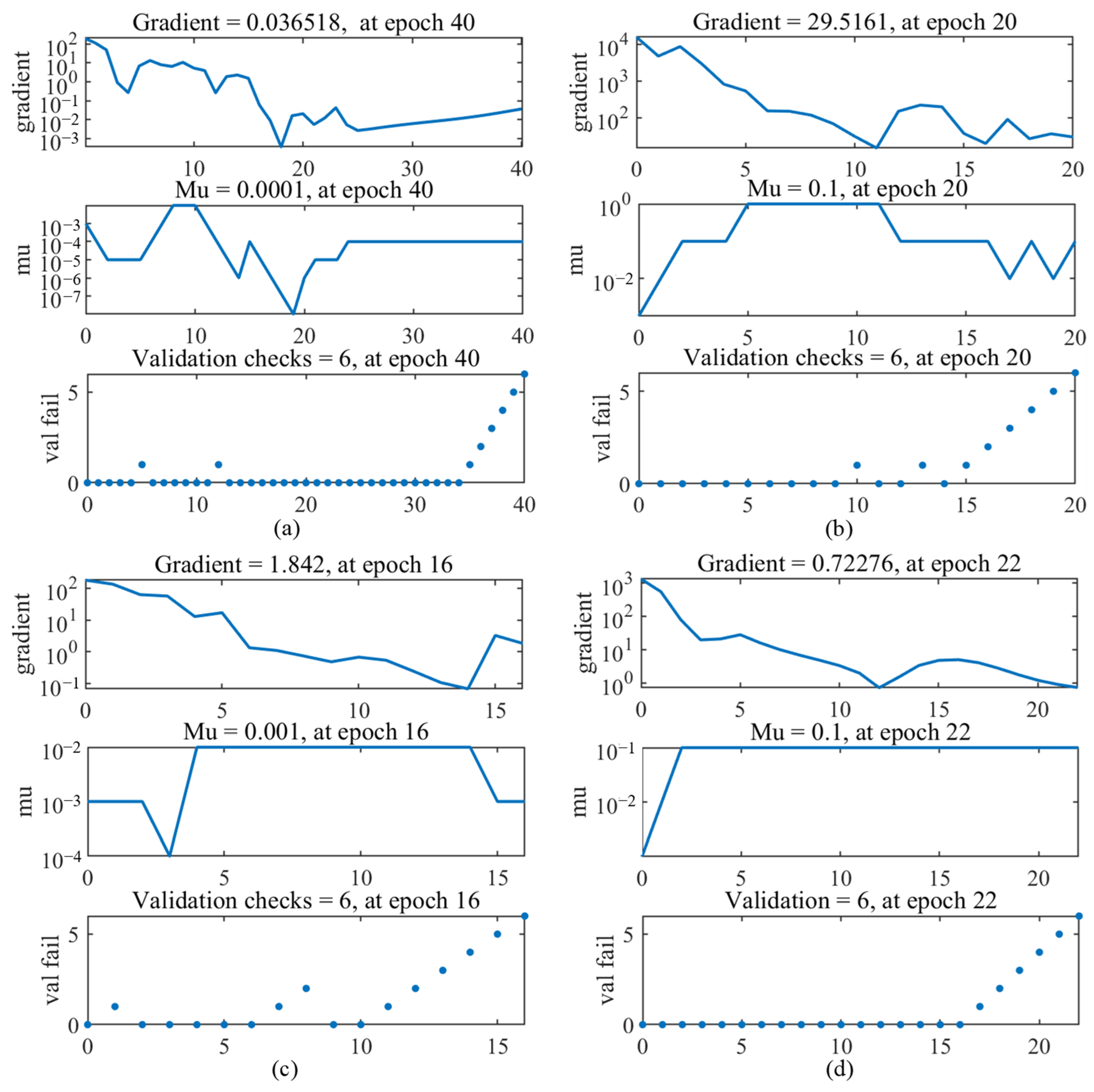
Figure 7 presents the training state diagrams of the four MLP models. Each diagram consists of three subgraphs, which collectively illustrate the relationship between the number of iterations and the training state of the learning function. The first subgraph depicts the variation in the gradient function value as the number of iteration steps increases. The second subgraph displays the relationship between the damping factor (mu) and the iteration steps. The third subgraph is a validation check graph; 0 indicates that the error continues to decrease during the training process. The training process is terminated if the error cannot be reduced after six consecutive training sessions. As the four MLP networks undergo training, the errors in their samples cease to decrease and, in some cases, even increase. This behavior suggests that the MLP models have reached their optimal performance levels. Continuing the training process beyond this point would not further reduce errors and could lead to overfitting.
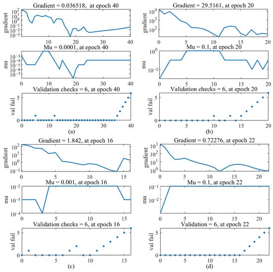
Figure 7.
MLP training state plots: (a) rime ice accretion mass MLP; (b) rime ice maximum ice thickness MLP; (c) glaze ice accretion mass MLP; and (d) glaze ice maximum ice thickness MLP.
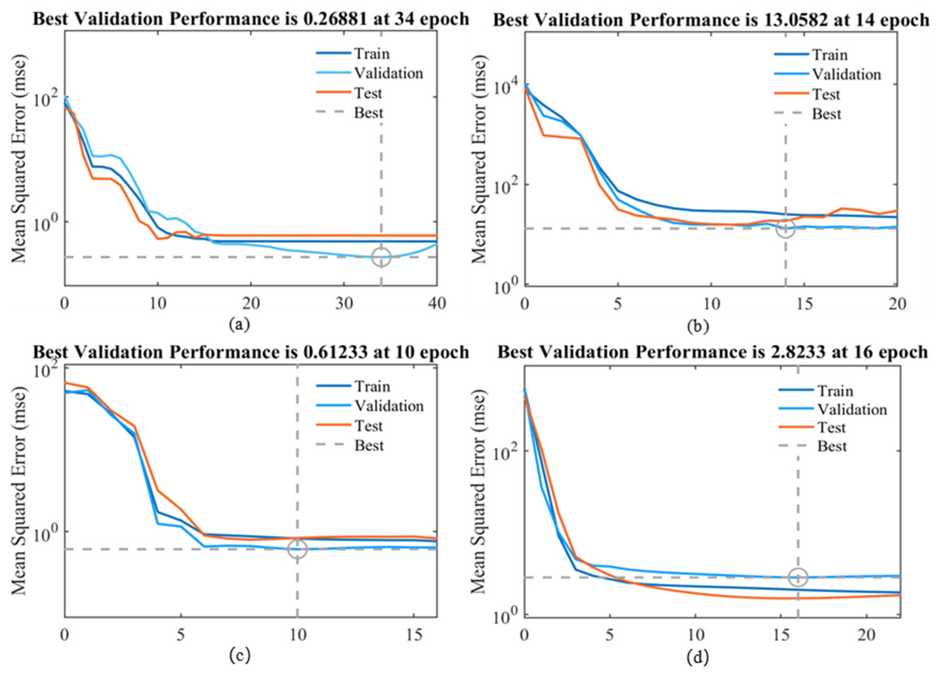
The convergence curve of the model is depicted in Figure 8, which also presents the optimal validation performance for each model. The primary objective of the training process is to obtain predicted outputs for all input values of the network while minimizing the error function. The network learns and adjusts the input weights through an iterative approach to achieve optimal training. In this study, a maximum of 1000 iterations were considered, and the error parameter of the network was defined as the MSE, calculated as the mean squared difference between the predicted output and the target value. The validation set was utilized to evaluate the model’s performance. The training was halted when the validation set’s accuracy peaked and showed no improvement over the subsequent six iterations, indicating that the model was well-trained. The goal was to minimize the average number of errors as much as possible, with lower values indicating better performance. One epoch represents that all training data is fully learned by the model once. If the MSE of the validation set decreases very little (below the preset threshold) in several consecutive iterations, the model is considered to have converged. If the validation set error starts to rise (overfitting), the iteration will also end at this epoch. A zero-error value would signify perfect prediction. The best dashed line in the figure represents the ideal result for the current training steps. Among the four models, the MSE values for the training, validation, and testing datasets generally decreased. These trends did not indicate overfitting, suggesting that the network was adequately trained and capable of generalizing well to unseen data.
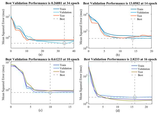
Figure 8.
MLP performance plots: (a) rime ice accretion mass MLP; (b) rime ice maximum ice thickness MLP; (c) glaze ice accretion mass MLP; and (d) glaze ice maximum ice thickness MLP.
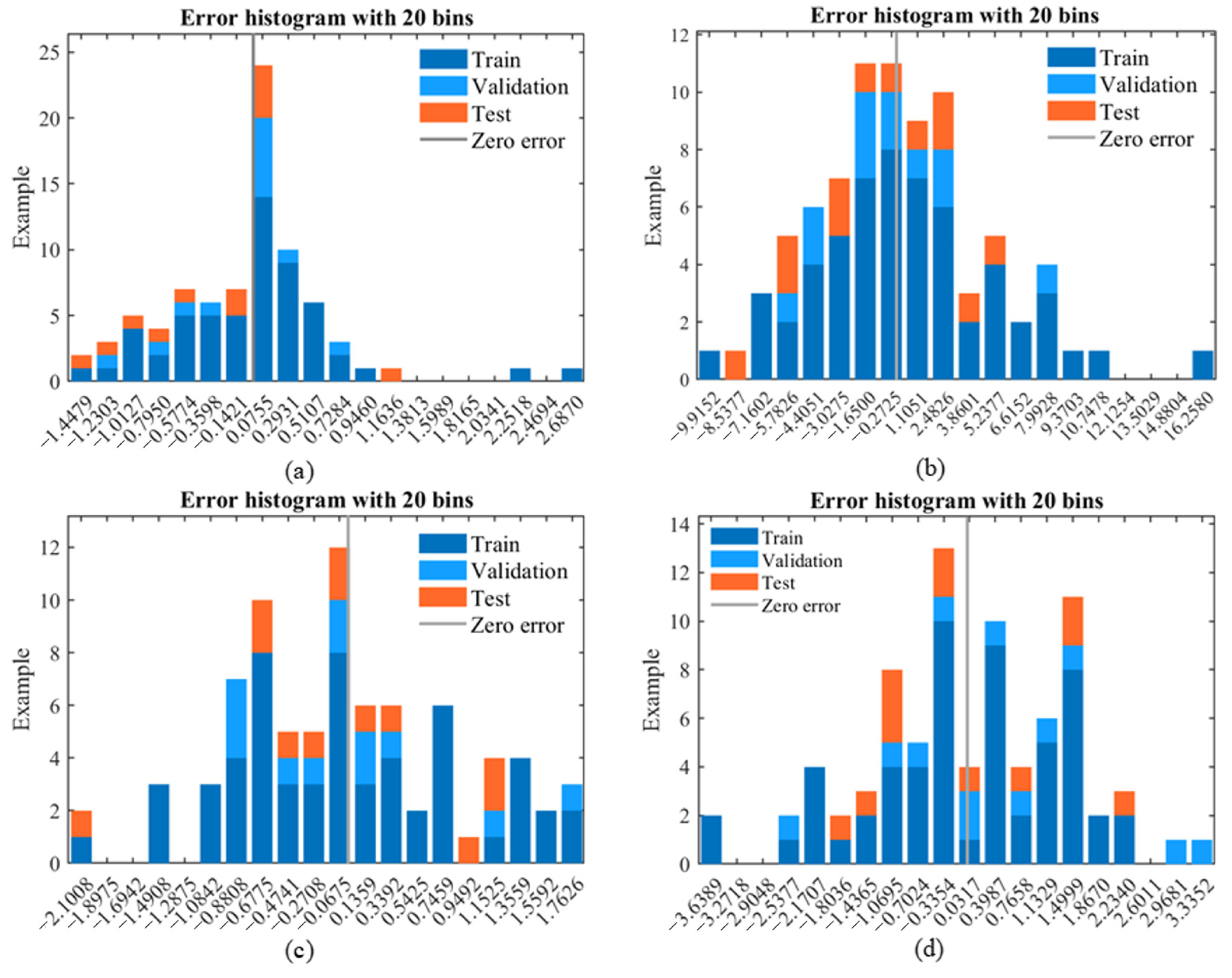
The error histograms for 20 intervals of each model are presented in Figure 9. The graphs reveal that the error values are predominantly close to zero, indicating that the discrepancy between the target and actual values of the model is minimal. The error distribution follows a normal distribution pattern characterized by symmetry and concentration around the mean (zero error). This suggests that the MLP network exhibits no significant bias or systematic error, and the model demonstrates strong performance on the test data, with small errors and no systematic deviations. These findings indicate that the prediction results of the model are highly reliable. Furthermore, from a distribution perspective, the error values of the MLP model for predicting rime ice mass are more tightly clustered around the zero-error line than those of the other models. This concentration of errors near zero suggests that the training effect of this particular model is the most effective among the four, highlighting its superior predictive capability for rime ice mass estimation.
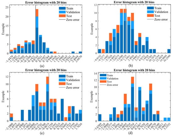
Figure 9.
MLP error histograms: (a) rime ice accretion mass MLP; (b) rime ice maximum ice thickness MLP; (c) glaze ice accretion mass MLP; and (d) glaze ice maximum ice thickness MLP.
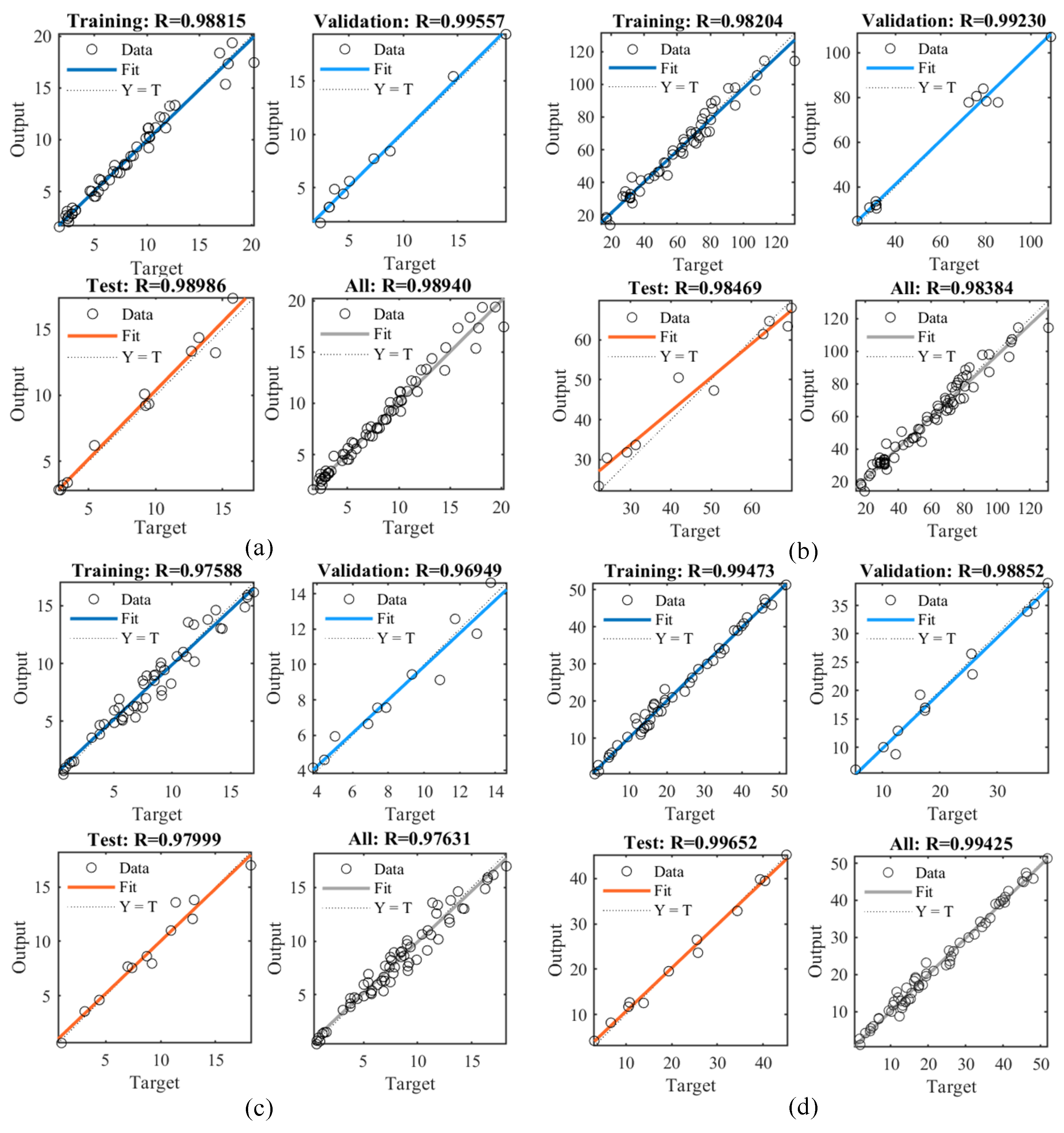
Figure 10 consists of four sets of scatter plots, each illustrating the correlation between the predicted and actual values for the four MLP models. Each set includes subplots representing the regression results for the training, validation, test, and combined datasets. The horizontal axis represents the actual values of the samples, while the vertical axis corresponds to the model-derived predictions. The R value, displayed in the figure, quantifies the strength of the relationship between the predicted and actual values for each dataset. An R value close to 1 indicates a strong agreement between the predicted and target values. The data points are clustered around the solid regression line, with the dotted line representing the ideal scenario where the predicted and actual values are identical, signifying perfect prediction. In an ideal case, if all points lie exactly on the dotted line, the R value would equal 1, indicating flawless estimation by the model with no errors. In Figure 10, the data points for all models are situated close to the dotted line, demonstrating satisfactory performance across the MLP models. Based on the R values for the combined datasets, the rime ice mass and maximum thickness models exhibit R values of 0.98940 and 0.98384, respectively. These values are higher than those of the glaze ice models, indicating a stronger correlation between the predicted and actual values for the rime ice models. This suggests that the rime ice models provide more accurate predictions than the glaze ice models, as reflected by their superior R values.
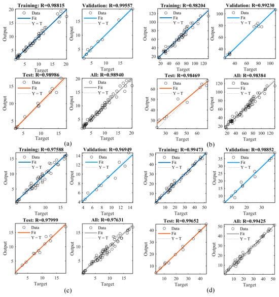
Figure 10.
MLP data regression plots: (a) rime ice accretion mass MLP; (b) rime ice maximum ice thickness MLP; (c) glaze ice accretion mass MLP; and (d) glaze ice maximum ice thickness MLP.
The calculation of the evaluation results uses all the data, as shown in Table 6.
Table 6.
MLP model performance evaluation results.
In terms of predicting the thickness and mass of rime ice, Table 6 shows that the MLP model performs well across all evaluation metrics. The MSE of rime ice mass is close to 0, while the MSE of rime thickness is slightly higher but still within a good range. The R2 values of both models exceed 0.96, indicating strong explanatory power and high consistency between the predicted and actual values. In addition, the MAPE of the two models is about 7%, which meets certain engineering accuracy requirements. Table 6 also shows that the MLP model performs well in all evaluation indicators of glaze ice. The MSE of glaze ice mass is close to 0, while the MSE of glaze ice thickness is slightly higher. The R2 values of both glaze ice models are above 0.95, indicating good explanatory power.
Based on all the data, the MAPE of the glaze ice model is slightly higher than that of the rime ice model. For this phenomenon, it is speculated that the formation mechanism of rime ice is relatively simpler than that of glaze ice, and the quality of rime ice data is better than that of glaze ice. It may also be due to limitations caused by limited training data. In addition, based on the MAPE results, the MLP model predicts the maximum ice thickness more accurately than the predicted mass. This phenomenon indicates that the model is particularly effective for thickness prediction, which may be attributed to the accumulation of ice at the leading edge of the blade, which extends towards the tail of the blade, making it difficult to predict the overall increase in mass. Overall, the MLP model has a strong predictive ability for rime and glaze ice mass and thickness.
4.3. Model Practicality
Based on climate data collected from a high-altitude wind farm during a long icing period, an MLP neural network is employed to predict future icing conditions on wind turbines. In order to cope with complex meteorological changes, the long icing period is divided into multiple smaller intervals, during which meteorological parameters are assumed to remain relatively stable. The meteorological parameters for each interval are input into the MLP prediction model to estimate the ice mass and maximum ice thickness for that specific period. The total ice accretion mass and the maximum ice thickness over the entire icing period can be obtained by aggregating the predicted ice accretion data from all intervals. This approach allows for a detailed and dynamic prediction of ice accumulation, accounting for variations in meteorological conditions across different time intervals, and provides valuable insights for managing ice-related challenges in wind farm operations.
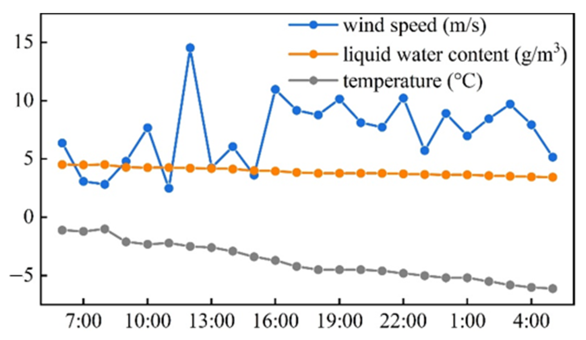
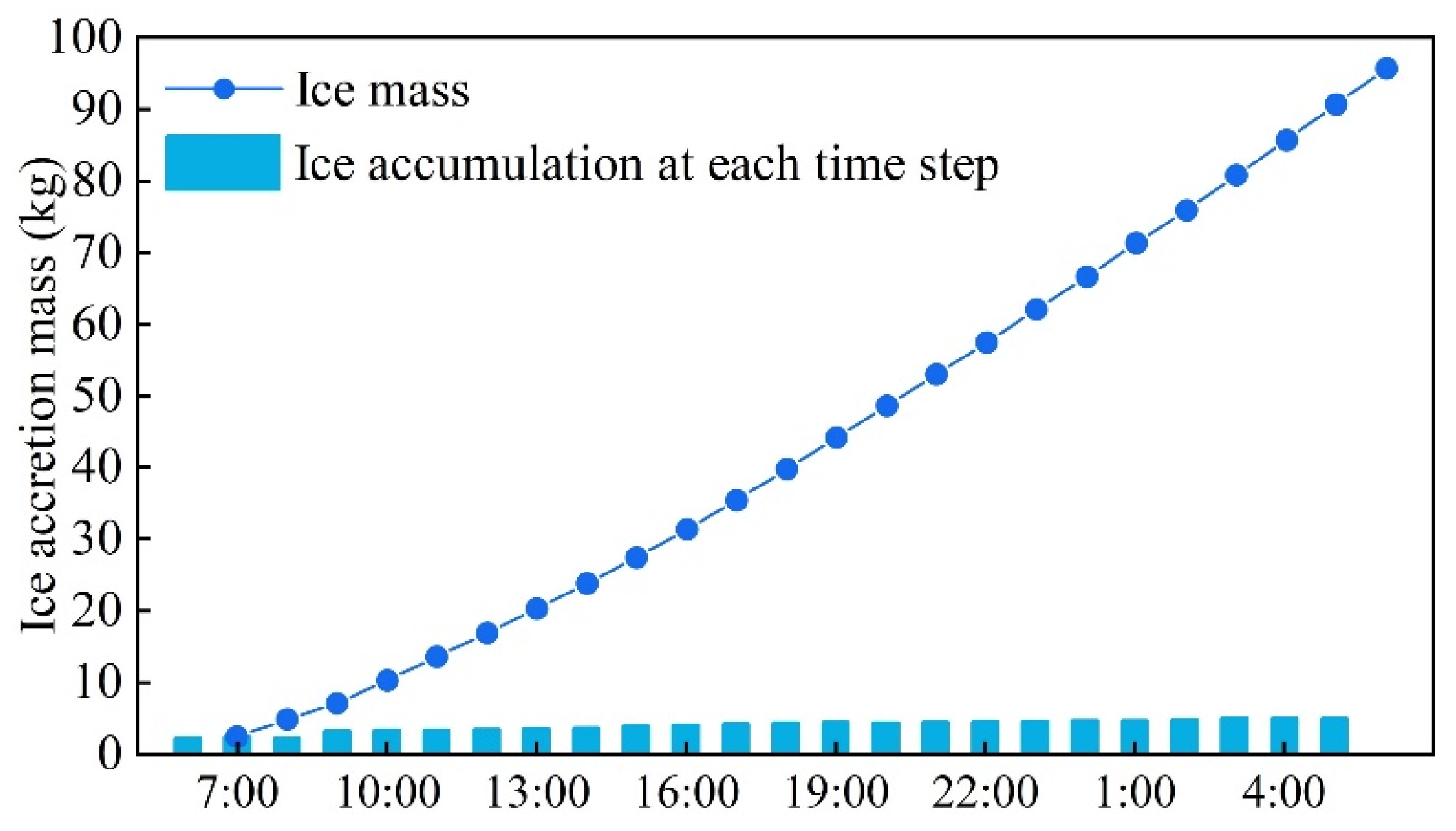
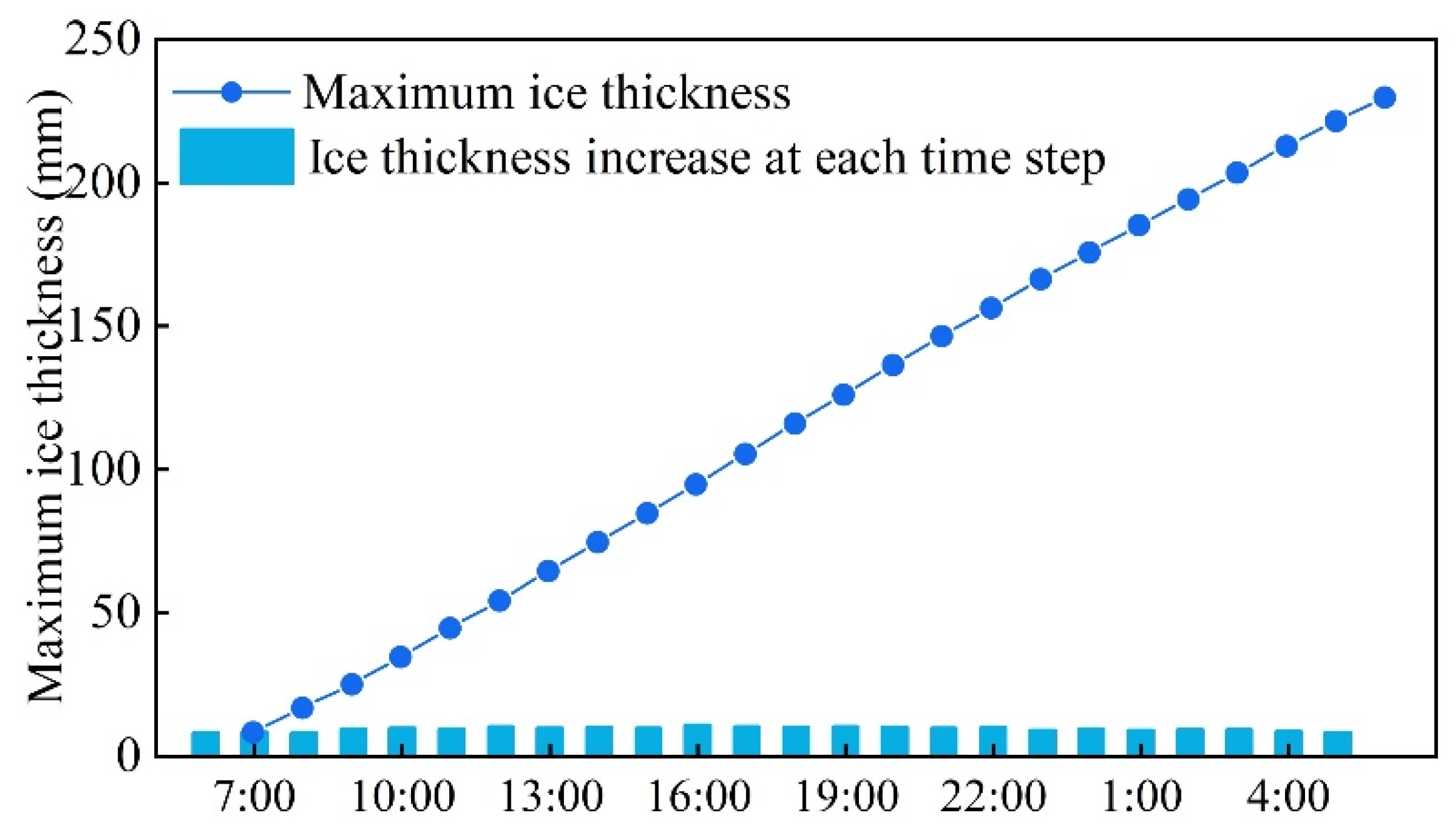
Figure 11 illustrates the variations in meteorological parameters during a long icing period, with data sourced from wind turbine sensors at a local wind farm located at 27° N and 117° E. As shown in Figure 11, the temperature around the wind turbine blades ranges from approximately −1 °C to −6 °C, which is the temperature for the formation of glaze ice. Consequently, the glaze ice prediction model was utilized for calculations, and the predicted results are presented in Figure 12 and Figure 13. In Figure 12 and Figure 13, the bar charts represent the incremental ice accretion from one time point to the next, while the line charts depict the cumulative ice accretion from the start of the period to the current time point. Figure 12 reveals that the maximum hourly ice accretion mass is 5.01 kg, with a cumulative ice mass of 95.43 kg over 24 h. Similarly, Figure 13 shows that the maximum hourly ice accretion thickness is 10.38 mm, with a cumulative ice thickness of 228.43 mm over the same 24 h period.
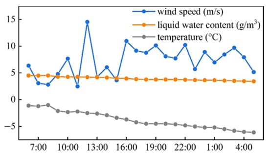
Figure 11.
Climate parameter change chart of a chosen wind farm.
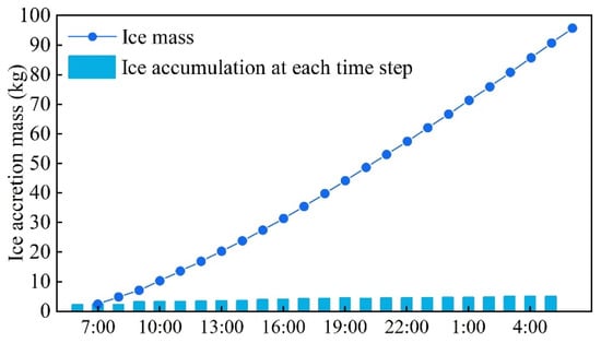
Figure 12.
Ice mass change chart of the blade.
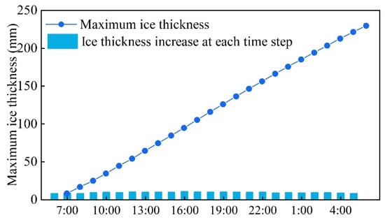
Figure 13.
Ice thickness change chart of the blade.
Based on the results presented, the MLP prediction model offers a significant advantage over conventional simulation methods by addressing the limitation of slow computational speed. Traditional numerical simulations for icing typically require more than half an hour to analyze a single simulation condition. In contrast, the MLP model can rapidly predict icing conditions on wind turbine blade surfaces within seconds by inputting key climatic parameters. This capability meets the critical need for real-time wind turbine blade icing prediction.
The swift and accurate predictions the MLP model provides enable wind farm operators to make timely adjustments to turbine operation strategies. Additionally, operators can effectively plan de-icing methods and allocate the necessary workforce in advance by monitoring ice accumulation and thickness variations. This proactive approach enhances operational efficiency and minimizes the risks associated with ice accumulation, such as reduced turbine performance or potential damage. Overall, the MLP model is a powerful tool for improving the safety and reliability of wind farm operations during icing conditions.
5. Conclusions
This work employs icing simulation data to train an MLP neural network, establishing a predictive model based on three key meteorological parameters: the temperature, LWC, and inflow velocity. The model is designed to predict the ice accretion mass and maximum ice thickness for both rime ice and glaze ice on the surface of wind turbine blades. This study also evaluates the performance of the optimally configured MLP model and demonstrates its application in a case study. The main conclusions are as follows:
- (1)
- Compared with traditional numerical model prediction, this method can quickly predict the mass and thickness of icing based on icing conditions, improving computational efficiency.
- (2)
- The constructed MLP model demonstrates strong predictive accuracy, with MAPE values of 7.13% for rime ice mass prediction and 7.02% for rime ice thickness. For glaze ice, the MAPE values are 10.22% for mass and 9.42% for thickness, indicating reliable performance across different icing types.
- (3)
- With R2 values exceeding 0.95 for all models, the results confirm the MLP neural network’s suitability for accurately predicting the icing process. This high level of agreement between the predicted and actual values underscores the model’s robustness.
- (4)
- The MLP neural network’s method for predicting the icing process shows strong potential for application in wind farms. It enables the rapid forecasting of blade icing conditions while maintaining prediction accuracy, even under fluctuating climatic parameters. This capability is of particular value in dealing with the challenges that climate variability poses to wind power generation.
Supplementary Materials
The following supporting information can be downloaded at: https://www.mdpi.com/article/10.3390/pr13061910/s1, Table S1: Simulation conditions.
Author Contributions
N.X.: methodology, investigation, and funding acquisition. Q.C.: writing—original draft—software. Z.Z.: conceptualization and resources. K.M.: visualization and validation. S.Z.: writing—review and editing—supervision. All authors have read and agreed to the published version of the manuscript.
Funding
This work was supported by the National Natural Science Foundation of China [grant number 52206037].
Data Availability Statement
The data that support the findings of this study can be made available by the corresponding author upon reasonable request.
Conflicts of Interest
The authors declare that they have no known competing financial interests or personal relationships that could have appeared to influence the work reported in this paper.
Nomenclature
| a | Number of hidden layer neurons |
| m | Number of input layer neurons |
| N | Total sample size |
| n | Number of output layer neurons |
| x | Input variable of the layer |
| Actual value of the i sample | |
| Predicted value of the i sample | |
| Mean of the actual value | |
| Mean of the predicted value | |
| α | Random constant |
| ANN | Artificial neural network |
| BP | Backpropagation |
| CFD | Computational Fluid Dynamics |
| DNN | Deep neural network |
| LM | Levenberg–Marquardt |
| LWC | Liquid water content |
| MAPE | Mean absolute percentage error |
| MLP | Multilayer Perceptron |
| MSE | Mean Squared Error |
| MVD | Median volume diameter |
| R | Pearson correlation coefficient |
| R2 | R-squared |
| SCG | Scaled Conjugate Gradient |
References
- Lamraoui, F.; Fortin, G.; Benoit, R.; Perron, J.; Masson, C. Atmospheric icing impact on wind turbine production. Cold Reg. Sci. Technol. 2014, 100, 36–49. [Google Scholar] [CrossRef]
- Ibrahim, G.M.; Pope, K.; Muzychka, Y.S. Effects of blade design on ice accretion for horizontal axis wind turbines. J. Wind Eng. Ind. Aerodyn. 2018, 173, 39–52. [Google Scholar] [CrossRef]
- Shu, L.; Li, H.; Hu, Q.; Jiang, X.; Qiu, G.; McClure, G.; Yang, H. Study of ice accretion feature and power characteristics of wind turbines at natural icing environment. Cold Reg. Sci. Technol. 2018, 147, 45–54. [Google Scholar] [CrossRef]
- Gao, L.; Dasari, T.; Hong, J. Wind farm icing loss forecast pertinent to winter extremes. Sustain. Energy Technol. Assess. 2022, 50, 101872. [Google Scholar] [CrossRef]
- Yirtici, O.; Tuncer, I.H. Aerodynamic shape optimization of wind turbine blades for minimizing power production losses due to icing. Cold Reg. Sci. Technol. 2021, 185, 103250. [Google Scholar] [CrossRef]
- Gao, L.; Liu, Y.; Ma, L.; Hu, H. A hybrid strategy combining minimized leading-edge electric-heating and superhydro-/ice-phobic surface coating for wind turbine icing mitigation. Renew. Energy 2019, 140, 943–956. [Google Scholar] [CrossRef]
- Wang, Z. Recent progress on ultrasonic de-icing technique used for wind power generation, high-voltage transmission line and aircraft. Energy Build. 2017, 140, 42–49. [Google Scholar] [CrossRef]
- Wang, Q.; Yi, X.; Liu, Y.; Ren, J.; Yang, J.; Chen, N. Numerical investigation of dynamic icing of wind turbine blades under wind shear conditions. Renew. Energy 2024, 227, 120495. [Google Scholar] [CrossRef]
- Dalili, N.; Edrisy, A.; Carriveau, R. A review of surface engineering issues critical to wind turbine performance. Renew. Sustain. Energy Rev. 2009, 13, 428–438. [Google Scholar] [CrossRef]
- Ye, F.; Ezzat, A.A. Icing detection and prediction for wind turbines using multivariate sensor data and machine learning. Renew. Energy 2024, 231, 120879. [Google Scholar] [CrossRef]
- Hu, Q.; Xu, X.; Leng, D.; Shu, L.; Jiang, X.; Virk, M.; Yin, P. A method for measuring ice thickness of wind turbine blades based on edge detection. Cold Reg. Sci. Technol. 2021, 192, 103398. [Google Scholar] [CrossRef]
- Sirui, Y.; Mengjie, S.; Runmiao, G.; Jiwoong, B.; Xuan, Z.; Shiqiang, Z. A review of icing prediction techniques for four typical surfaces in low-temperature natural environments. Appl. Therm. Eng. 2024, 241, 122418. [Google Scholar] [CrossRef]
- Bose, N. Icing on a small horizontal-axis wind turbine—Part 1: Glaze ice profiles. J. Wind Eng. Ind. Aerodyn. 1992, 45, 75–85. [Google Scholar] [CrossRef]
- Fu, P.; Farzaneh, M. A CFD approach for modeling the rime-ice accretion process on a horizontal-axis wind turbine. J. Wind Eng. Ind. Aerodyn. 2010, 98, 181–188. [Google Scholar] [CrossRef]
- Han, Y.; Palacios, J.; Schmitz, S. Scaled ice accretion experiments on a rotating wind turbine blade. J. Wind Eng. Ind. Aerodyn. 2012, 109, 55–67. [Google Scholar] [CrossRef]
- Wang, Q.; Yi, X.; Liu, Y.; Ren, J.; Li, W.; Wang, Q.; Lai, Q. Simulation and analysis of wind turbine ice accretion under yaw condition via an Improved Multi-Shot Icing Computational Model. Renew. Energy 2020, 162, 1854–1873. [Google Scholar] [CrossRef]
- Chuang, Z.; Li, C.; Liu, S.; Li, X.; Li, Z.; Zhou, L. Numerical analysis of blade icing influence on the dynamic response of an integrated offshore wind turbine. Ocean Eng. 2022, 257, 111593. [Google Scholar] [CrossRef]
- Chuang, Z.; Yi, H.; Chang, X.; Liu, H.; Zhang, H.; Xia, L. Comprehensive Analysis of the Impact of the Icing of Wind Turbine Blades on Power Loss in Cold Regions. J. Mar. Sci. Eng. 2023, 11, 1125. [Google Scholar] [CrossRef]
- Ibrahim, G.M.; Pope, K.; Naterer, G.F. Extended scaling approach for droplet flow and glaze ice accretion on a rotating wind turbine blade. J. Wind Eng. Ind. Aerodyn. 2023, 233, 105296. [Google Scholar] [CrossRef]
- Ibrahim, G.M.; Pope, K.; Naterer, G.F. Scaling formulation of multiphase flow and droplet trajectories with rime ice accretion on a rotating wind turbine blade. J. Wind Eng. Ind. Aerodyn. 2023, 232, 105247. [Google Scholar] [CrossRef]
- Cao, H.Q.; Bai, X.; Ma, X.D.; Yin, Q.; Yang, X.Y. Numerical Simulation of Icing on Nrel 5-MW Reference Offshore Wind Turbine Blades Under Different Icing Conditions. China Ocean Eng. 2022, 36, 767–780. [Google Scholar] [CrossRef]
- Shu, L.; Liang, J.; Hu, Q.; Jiang, X.; Ren, X.; Qiu, G. Study on small wind turbine icing and its performance. Cold Reg. Sci. Technol. 2017, 134, 11–19. [Google Scholar] [CrossRef]
- Li, T.; Xu, J.; Liu, Z.; Wang, D.; Tan, W. Detecting Icing on the Blades of a Wind Turbine Using a Deep Neural Network. CMES-Comput. Model. Eng. Sci. 2022, 134, 767–782. [Google Scholar] [CrossRef]
- Kreutz, M.; Ait Alla, A.; Lütjen, M.; Ohlendorf, J.H.; Freitag, M.; Thoben, K.D.; Zimnol, F.; Greulich, A. Ice prediction for wind turbine rotor blades with time series data and a deep learning approach. Cold Reg. Sci. Technol. 2023, 206, 103741. [Google Scholar] [CrossRef]
- LB Effects and Prevention Systems of Icing on Wind Turbines in Cold Climates; Mechanical Industry Press: Beijing, China, 2022.
- Guo, W.; Shen, H.; Li, Y.; Feng, F.; Tagawa, K. Wind tunnel tests of the rime icing characteristics of a straight-bladed vertical axis wind turbine. Renew. Energy 2021, 179, 116–132. [Google Scholar] [CrossRef]
- Xu, Z.; Zhang, T.; Li, X.; Li, Y. Effects of ambient temperature and wind speed on icing characteristics and anti-icing energy demand of a blade airfoil for wind turbine. Renew. Energy 2023, 217, 119135. [Google Scholar] [CrossRef]
- Homola, M.C.; Virk, M.S.; Wallenius, T.; Nicklasson, P.J.; Sundsbø, P.A. Effect of atmospheric temperature and droplet size variation on ice accretion of wind turbine blades. J. Wind Eng. Ind. Aerodyn. 2010, 98, 724–729. [Google Scholar] [CrossRef]
- Li, Y.; Tagawa, K.; Feng, F.; Li, Q.; He, Q. A wind tunnel experimental study of icing on wind turbine blade airfoil. Energy Convers. Manag. 2014, 85, 591–595. [Google Scholar] [CrossRef]
- Lisheng, M.; He, S.; Yan, C.; Huanyu, D.; Xiaofeng, L. A numerical simulation of the distribution and the variation law of the liquid water content in icing wind tunnel. Appl. Therm. Eng. 2024, 236, 121539. [Google Scholar] [CrossRef]
- Cao, Y.; Tan, W.; Wu, Z. Aircraft icing: An ongoing threat to aviation safety. Aerosp. Sci. Technol. 2018, 75, 353–385. [Google Scholar] [CrossRef]
- Han, Y.; Palacios, J.; Smith, E. An Experimental Correlation Between Rotor Test and Wind Tunnel Ice Shapes on NACA 0012 Airfoils2011; No. 2011-38-0092 SAE Technical Paper; SAE International: Warrendale, PA, USA, 2011. [Google Scholar]
- Emambocus, B.A.S.; Jasser, M.B.; Amphawan, A. A Survey on the Optimization of Artificial Neural Networks Using Swarm Intelligence Algorithms. IEEE Access 2023, 11, 1280–1294. [Google Scholar] [CrossRef]
- Cong, T.; Su, G.; Qiu, S.; Tian, W. Applications of ANNs in flow and heat transfer problems in nuclear engineering: A review work. Prog. Nucl. Energy 2013, 62, 54–71. [Google Scholar] [CrossRef]
- Ding, L. Human Knowledge in Constructing AI Systems—Neural Logic Networks Approach towards an Explainable AI. Procedia Comput. Sci. 2018, 126, 1561–1570. [Google Scholar] [CrossRef]
- Zarei, T.; Behyad, R. Predicting the water production of a solar seawater greenhouse desalination unit using multi-layer perceptron model. Sol. Energy 2019, 177, 595–603. [Google Scholar] [CrossRef]
- Tao, P.; Cheng, J.; Chen, L. Brain-inspired chaotic backpropagation for MLP. Neural Netw. 2022, 155, 1–13. [Google Scholar] [CrossRef]
- Hamed, M.M.; Khalafallah, M.G.; Hassanien, E.A. Prediction of wastewater treatment plant performance using artificial neural networks. Environ. Model. Softw. 2004, 19, 919–928. [Google Scholar] [CrossRef]
- Yuan, E. Artificial Neural Networks and Their Applications; Tsinghua University Press: Beijing, China, 1999. [Google Scholar]
- Hemmati-Sarapardeh, A.; Varamesh, A.; Husein, M.M.; Karan, K. On the evaluation of the viscosity of nanofluid systems: Modeling and data assessment. Renew. Sustain. Energy Rev. 2018, 81, 313–329. [Google Scholar] [CrossRef]
- Bayrak, G.; Yılmaz, A.; Çalışır, A. A new intelligent decision-maker method determining the optimal connection point and operating conditions of hydrogen energy-based DGs to the main grid. Int. J. Hydrogen Energy 2023, 48, 23168–23184. [Google Scholar] [CrossRef]

Disclaimer/Publisher’s Note: The statements, opinions and data contained in all publications are solely those of the individual author(s) and contributor(s) and not of MDPI and/or the editor(s). MDPI and/or the editor(s) disclaim responsibility for any injury to people or property resulting from any ideas, methods, instructions or products referred to in the content. |
© 2025 by the authors. Licensee MDPI, Basel, Switzerland. This article is an open access article distributed under the terms and conditions of the Creative Commons Attribution (CC BY) license (https://creativecommons.org/licenses/by/4.0/).