Dynamic Modeling of Heat-Integrated Air Separation Column Based on Nonlinear Wave Theory and Mass Transfer Mechanism

Abstract

The air separation process is an important industrial process for the production of high-purity nitrogen and oxygen, representing the level of technological development in a country’s chemical industry. It has high energy consumption but very low energy utilization efficiency. In the overall environment of increasingly scarce global energy, the application of internal heat coupling technology in the air separation process can effectively reduce energy consumption. However, due to the low-temperature characteristics, ultra-high purity characteristics, and the nature of multi-component systems of the heat-integrated air separation column (HIASC), its modeling process and dynamic characteristic analysis are complex. To solve the disadvantages of overly complex mechanistic models and insufficient accuracy of traditional simplified models, a concentration distribution curve description method based on the mass transfer mechanism is proposed, and combined with the traditional wave theory, a nonlinear wave model of the HIASC is established. Based on this model, static and dynamic analyses were carried out, and the research results prove that the newly established nonlinear wave model maintains high accuracy while simplifying the model complexity. It can not only accurately track the concentration changes of key products but also fully reflect various typical nonlinear characteristics of the system. Compared to the mechanism model, the wave model can reduce the running time by approximately 20%, thereby improving operational efficiency. This method explains various characteristics of the system from a perspective different from that of the mechanistic model.

1. Introduction

The air separation process is a process of separating nitrogen and oxygen or simultaneously extracting rare gases, such as argon, from the air by utilizing the differences in physical properties of air components through technologies such as adsorption, membrane separation, and cryogenic separation [1,2]. The products produced by the air separation process have a wide range of applications and are suitable for many industries, such as new energy, scientific research, environmental protection, national defense, aerospace, etc. [3,4,5]. The air separation process usually employs various methods, including cryogenic distillation, pressure swing adsorption, membrane permeation, etc. Among them, cryogenic distillation is the most widely used [6,7,8,9]. The cryogenic distillation technique can simultaneously produce high-purity nitrogen and oxygen in the air separation tower, meeting the nitrogen and oxygen requirements of industrial processes such as steelmaking and metallurgy [10,11,12]. This technique has significant advantages in the air separation process; thus, the research in this paper is also based on this technique [13,14,15,16]. However, the cryogenic distillation technique has high energy consumption and low energy utilization efficiency, and how to improve the energy utilization efficiency of the air separation process is a research hotspot in this field [17].

The internal heat integration technology shows obvious energy-saving advantages in the distillation process, and the air separation process is a unique cryogenic distillation method [18,19,20]. Therefore, applying heat-integrating technology to the air separation process can greatly improve energy utilization efficiency, which is of great significance and can bring considerable economic benefits to industrial production [21,22,23,24]. In recent years, some experts have already achieved certain research results in the construction and improvement of models of the heat-integrated air separation column (HIASC) [25,26,27]. Yan proposed a mechanistic model of the HIASC, and the research results show that compared with the conventional air separation column, the proposed model has a better separation effect, and the energy-saving potential of the HIASC has increased by about 47% [28]. Ham believes that using thermally coupled trays is the most promising method to improve the thermodynamic performance of traditional air separation columns compared with adding additional heat exchangers [29]. Chang proposed a new structure of an ideal HIASC and provided a rigorous mathematical model and parameter analysis. In addition, Chang also established an optimization model of operating parameters, and the new HIASC has a higher product acquisition rate and energy utilization rate [30].

In recent years, the nonlinear wave theory has played an important role in the nonlinear dynamic modeling and control scheme design of separation processes and has attracted the attention of a large number of scholars. The wave phenomenon is widespread in the separation field; that is, a certain parameter distribution propagates at a constant shape and speed during the transition process [31]. For distillation processes and air separation processes, there is also a constant waveform phenomenon described by the wave theory. Scholars such as Luyben and Hwang have conducted extensive research on the propagation and movement of waveforms in towers. This research perspective provides a completely new perspective for depicting the nonlinear dynamic processes of distillation and air separation processes and brings more possibilities for establishing nonlinear dynamic models [32,33,34]. Kienle proposed a new research method for low-order dynamic models of multi-component distillation processes based on the wave theory [35]. By comparing the differences between traditional models and the proposed nonlinear models under multi-component mixtures, the results show that the dynamic characteristics of the low-order wave model are consistent with the reference model under a large number of working conditions. The scalability of this method in terms of variable molar flow rate and variable volatility was also discussed. Liu explored the physical method of the internal heat-integrated distillation process based on the nonlinear wave theory [36]. On the basis of considering this improvement, a complete nonlinear wave model of the internal heat-integrated distillation column was established. The research results prove that the wave theory can play an active role in the heat-integrated distillation column.

At present, certain progress has been made in applying the wave theory to the nonlinear dynamic modeling of the HIASC. Fu derived the single-plate wave velocity of component concentration in the HIASC based on the wave theory, conducted relevant wave characteristic analysis, further derived the whole-column wave velocity of component concentration from a macroscopic perspective, and established a wave model based on the whole-column wave velocity of component concentration by introducing an empirical function of the concentration waveform, that is, the wave concentration distribution description function, and observed the dynamic characteristics. Considering that the waveform propagation process is not completely invariant, the corrected whole-column wave velocity equation of component concentration was derived, and on this basis, a wave model was established, and the dynamic characteristics were analyzed to prove the validity of the wave model [37]. However, the HIASC has a complex structure, and the separation object is a multi-component non-ideal air system, while this model still uses some of the wave theory of the ideal binary mixture system in the description of concentration distribution and wave velocity, which will have a certain impact on the model accuracy.

In this work, we take the wave model established by Fu [37] as the reference object for comparison and focus on solving the problem of its insufficiently detailed description of the air separation process. First, according to the mass transfer mechanism of the distillation process, the concentration distribution description function of the heat-integrated air separation process is re-derived to make it more suitable for complex non-ideal systems. Then, based on the new concentration distribution description function and the component concentration equilibrium relationship, a new concentration distribution curve movement function, that is, the wave velocity description function, is derived. Finally, based on the newly derived concentration distribution description function and wave velocity function, a nonlinear wave model of the HIASC is established, and detailed model analysis is performed. The simulation results show that the established model can maintain high model accuracy while simplifying the model structure and can provide effective help for subsequent system analysis, state estimation, and control design research.

2. Nonlinear Wave Modeling of the HIASC Based on Mass Transfer Mechanism

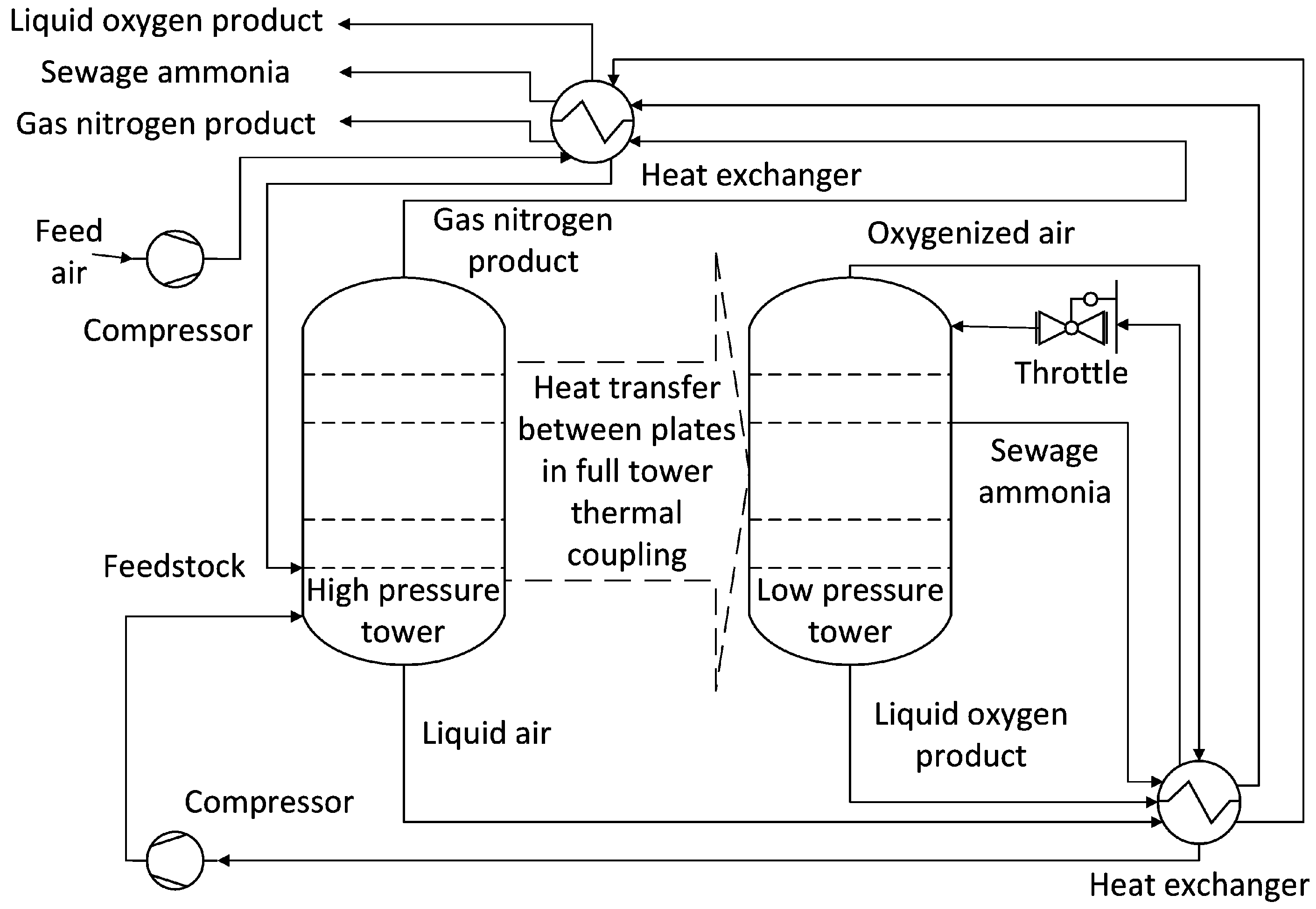
Figure 1 shows the structural diagram of the HIASC, which was created using Visio software (Visio 2021). The separation process is mainly completed by the rectifying section, stripping section, heat-coupling device, auxiliary condenser, throttle valve, and auxiliary reboiler. Among them, the auxiliary condenser and auxiliary reboiler are mainly put into use during the startup phase of the device, and the interaction between devices can be ignored during normal operation. Therefore, the auxiliary condenser and auxiliary reboiler are not drawn in the figure.

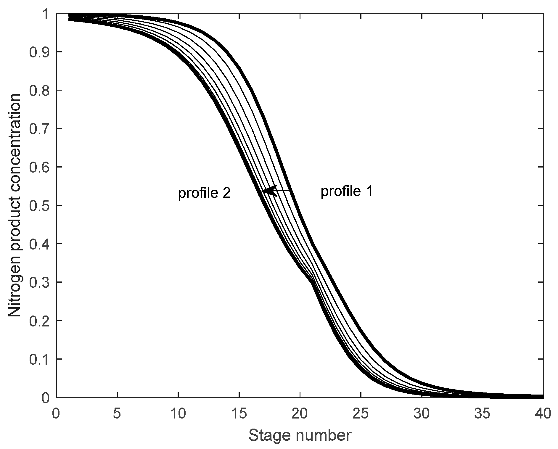
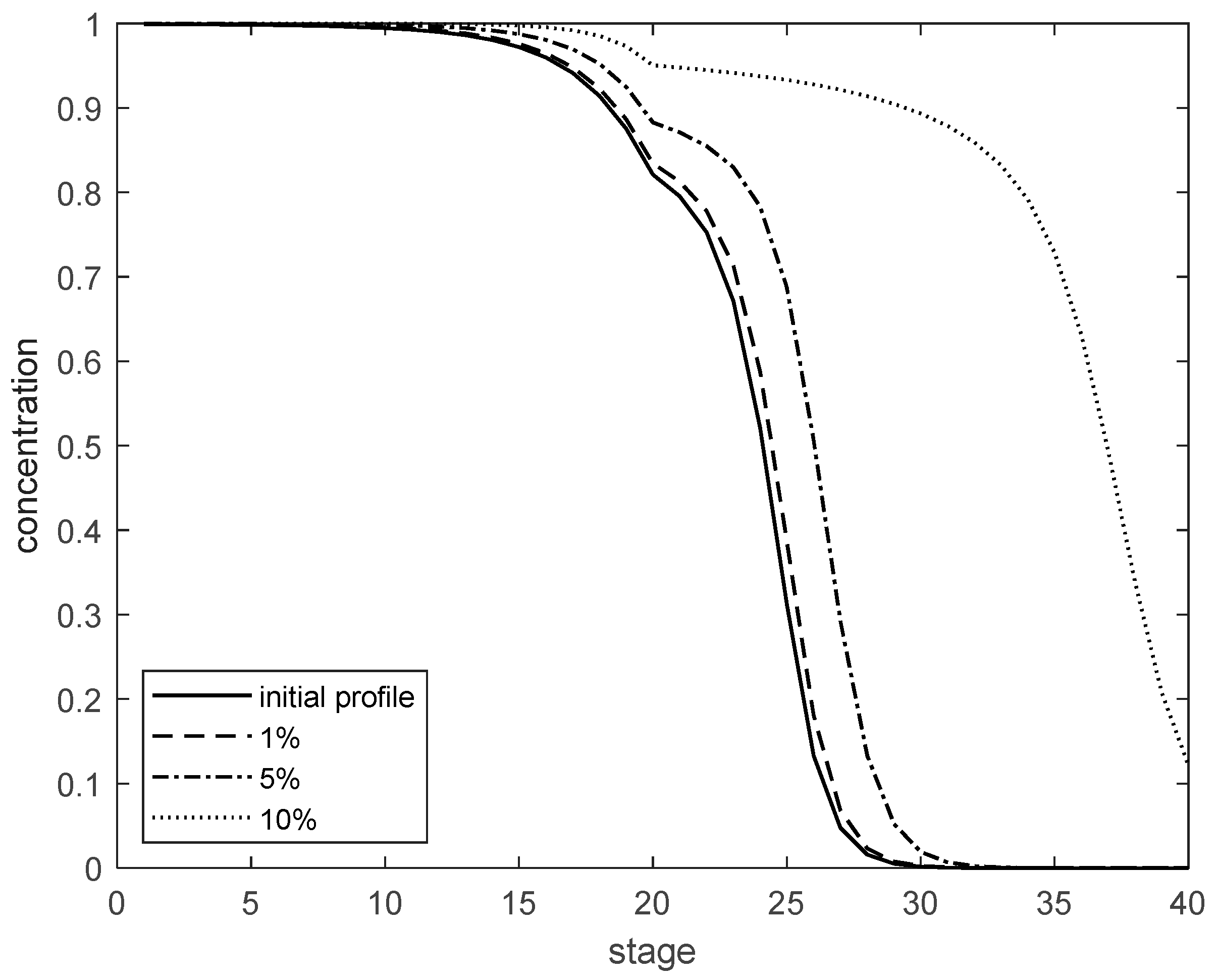
In the nonlinear wave theory [33], the concentration distribution can be regarded as a whole in the air separation column. When the operating conditions change, the concentration distribution curve moves as a whole in the air separation column. For example, Figure 2 shows the movement of the concentration distribution curve when the operating conditions change, which was created using Matlab software (Matlab 2024a). The original equilibrium state is profile1, and it moves to the left after the operating conditions change, finally stopping at the position of profile2. During the change process, the contour shape of the curve maintains a relatively stable structure. The movement process of the concentration distribution curve represents the dynamic response process of the entire system after the operating conditions change.

The traditional nonlinear wave model evolved from the conventional air separation tower to the HIASC [36,37]. Although it takes some typical features of the internal heat-coupled air separation tower into account, it does not conduct further research on the mass transfer mechanism of the HIASC. Its concentration distribution description function adopts a data-based identification method, so its accuracy is relatively insufficient. The concentration distribution description function is a core component of establishing the wave model. Therefore, to improve the accuracy of the nonlinear wave model, it is first necessary to further refine the concentration distribution description function through the study of the mass transfer mechanism of the HIASC to improve its description accuracy.

To simplify the process of solving the nonlinear asymptotic dynamic solution of the partial differential equation, we do not consider factors such as energy conservation and gas phase holdup. First, we start with the simple mass transfer partial differential equation within a very small unit volume in the air separation process [38], as shown below:

$${\displaystyle \frac{\partial x_i}{\partial t}}-{\displaystyle \frac{\partial x_i}{\partial s}}=-MT({y_i}^{*}\left(x_i\right)-y_i)$$

(1)

$${\displaystyle \frac{V}{L}}{\displaystyle \frac{\partial y_i}{\partial s}}=MT({y_i}^{*}\left(x_i\right)-y_i)$$

(2)

where $x_i$ and $y_i$ are the liquid-phase and gas-phase concentrations, respectively. $MT$ is the dimensionless mass transfer coefficient, $V$ is the gas-phase molar flow rate, $L$ is the liquid-phase molar flow rate, ${y_{\mathrm{i}}}^{\ast }\left(x_i\right)$ describes the gas–liquid equilibrium relationship, t represents time, s is the dimensionless spatial coordinate variable (the tray positions within the distillation column), and the subscript i represents different components such as oxygen, nitrogen, and argon.

We assume that the process is in a stable state, that is, ∂x/∂t = 0, and then perform integral transformation on Equation (1) to convert the original coordinate system into the l-t sub-coordinate system with the motion rate of v. The following is the coordinate transformation:

$$\epsilon =s-s^{\prime }$$

(3)

$$s^{\prime }=\int vdt$$

(4)

Substituting Equations (3) and (4) into Equations (1) and (2), we obtain

$$(1+v){\displaystyle \frac{\partial x_i}{\partial \epsilon }}=MT({y_i}^{*}\left(x_i\right)-y_i)$$

(5)

$${\displaystyle \frac{V}{L}}(1+v){\displaystyle \frac{\partial y_i}{\partial \epsilon }}=MT({y_i}^{*}\left(x_i\right)-y_i)$$

(6)

From Equations (5) and (6), we can easily derive the expression of Equation (7), that is,

$$\epsilon -\int {\displaystyle \frac{(1+v)dx}{MT(C_1+{y_i}^{*}\left(x_i\right)-L{x}_i/v)}}+C_2=0$$

(7)

Here, C₁ and C₂ are the constant terms generated by the indefinite integrals of Equations (5) and (6). It is difficult to solve for X ($\epsilon$) from Equation (7). In order to solve for X ($\epsilon$), the fractional function ${y_i}^{*}\left(x_i\right)={\displaystyle \frac{x_i+a}{b{x}_i+c}}$ is used to approximate the gas–liquid equilibrium relationship ${y_i}^{*}\left(x_i\right)$. The integrand in Equation (7) is processed by completing the square method as follows:

$${\displaystyle \frac{(1+v)}{MT(C_1+{y_i}^{*}\left(x_i\right)-L{x}_i/v)}}={\displaystyle \frac{x_i-m_4}{m_3(x_i-m_1)(x_i-m_2)}}$$

(8)

where $m_1$, $m_2$, $m_3$, and $m_4$ are represented as factorization parameters.

Applying Equation (8) to Equation (7) for integral operation, we can obtain the solution equation of X ($\epsilon$) as follows:

$$\epsilon -{\displaystyle \frac{1}{m_3\left(m_1-m_2\right)}}\left[\left(m_4+m_1\right)\ln \left(m_1-x_i\right)-\left(m_4+m_2\right)\ln \left(x_i-m_2\right)\right]-m_5=0$$

(9)

According to the coordinate transformation relationship described in Equation (3), and letting S = S’ + $m_5$, and γ = $m_3$($m_2$−$m_1$), the concentration distribution description function is as follows:

$$\epsilon +{\displaystyle \frac{1}{\gamma }}\left[\left(m_4+m_1\right)\ln \left(m_1-x_i\right)-\left(m_4+m_2\right)\ln \left(x_i-m_2\right)\right]-S=0$$

(10)

In the highly nonlinear distillation separation process, the propagation pattern of the concentration curve remains basically stable, that is, the shape of the concentration curve in the dynamic process is approximately in a stable state, and the time variation of $m_5$ is not significant, which indicates that there is the following approximate wave velocity relationship:

$${\displaystyle \frac{dS}{dt}}={\displaystyle \frac{d{S}^{\prime }}{dt}}=v$$

(11)

The concentration distribution description function (9) derived from the simplified mass transfer partial differential equation and the gas–liquid equilibrium relationship has relatively wide applicability because the distribution parameters $m_1$, $m_2$, γ, and $m_4$ have practical physical meanings, and S characterizes the position of the inflection point. Subsequent research results prove that using the asymptotic solution form shown in (9) to describe the shape of the concentration curve with asymptotic characteristics and inflection point properties can achieve higher accuracy. According to the calculation of Equation (10), the values of $m_1$, $m_2$, γ, and $m_4$ can be observed online using the least squares method. Equation (11) also represents the moving speed of the concentration curve, which can be characterized by the moving speed of the inflection point position S.

According to Equation (10), the concentration distribution description functions of the rectifying section and the stripping section of the HIASC are as follows:

$$j+{\displaystyle \frac{1}{k_r}}\left[\left(a_r+X_{i,r\_max}\right)\ln \left(X_{i,r\_max}-{\widehat{X}}_{i,j}\right)-\left(a_r+X_{i,r\_min}\right)\ln \left({{\widehat{X}}_{i,j}-X}_{i,r\_min}\right)\right]-S_r=0,j=\mathrm{1,2},\dots ,n/2,$$

(12)

$$j+{\displaystyle \frac{1}{k_s}}\left[\left(a_s+X_{i,s\_max}\right)\ln \left(X_{i,s\_max}-{\widehat{X}}_{i,j}\right)-\left(a_s+X_{i,s\_min}\right)\ln \left({{\widehat{X}}_{i,j}-X}_{i,s\_min}\right)\right]-S_s=0,j=f,f+1,\dots ,n$$

(13)

${\widehat{X}}_{i,j}$ is the observed concentration value on the j-th tray. $X_{i,r\_max}$, $X_{i,r\_min}$, $k_r$, $a_r$, $X_{i,s\_max}$, $X_{i,s\_min}$, $k_s$, and $a_s$ are waveform parameters. $S_r$ and $S_s$ represent the inflection point positions of the concentration distribution in the rectifying section and the stripping section, respectively. The distribution parameters have physical meanings, where $X_{i,r\_min}$ and $X_{i,s\_min}$ are the minimum approximation concentrations of the rectifying section and the stripping section, respectively. $k_r$ and $k_s$ are the slope characterization quantities of the inflection point positions, representing the magnitude of the slope at the inflection point position but not equal to the slope. $X_{i,r\_max}$ and $X_{i,s\_max}$ are the maximum approximation concentrations of the rectifying section and the stripping section, respectively. $a_r$ and $a_s$ characterize the asymmetry of the concentration distribution curves of the rectifying section and the stripping section, respectively.

The values of quasi-steady-state distribution parameters and inflection point positions can be obtained by solving the following problem using the least squares method as follows:

$$Min{\sum }_{j=1}^n{({\widehat{X}}_{i,j}-X_{i,j})}^2$$

(14)

By combining the concentration distribution description function with the material conservation equation, the velocity formula describing the dynamic characteristics can be derived. The material conservation relationship at each tray of the HIASC is shown as follows:

$$H{\displaystyle \frac{d{X}_{i,1}}{dt}}=-(V_1+G_1)y_{i,1}-{(L}_1+U_1)x_{i,1}+V_2{y}_{i,2}+F_1{z}_{i,1}$$

(15)

$$H{\displaystyle \frac{d{X}_{i,j}}{dt}}=L_{j-1}{x}_{i,j-1}-(V_j+G_j)y_{i,j}-{(L}_j+U_j)x_{i,j}+V_{j+1}{y}_{i,j+1}+F_j{z}_{i,j}$$

(16)

$$H{\displaystyle \frac{d{X}_{i,n}}{dt}}=L_{j-1}{x}_{i,j-1}-(V_j+G_j)y_{i,j}-{(L}_j+U_j)x_{i,j}+F_j{z}_{i,j}$$

(17)

where i and j represent different types of gases (such as oxygen, nitrogen, argon) and the number of trays, respectively. n refers to the total number of trays. H represents the holdup of each tray. x and y are the liquid-phase component concentration and gas-phase component concentration in each tray, respectively. L and V correspond to the molar flow rates of liquid and gas, respectively. G refers to the gas draw-off flow rate, U is the liquid draw-off flow rate, F is the total flow rate entering the system, and finally, z indicates the composition concentration.

During the dynamic process, the concentration distribution parameters, such as $X_{i,r\_max}$, $X_{i,r\_min}$, $k_r$, $a_r$, $X_{i,s\_max}$, $X_{i,s\_min}$, $k_s,$ and $a_s,$ do not fluctuate significantly. Therefore, we can assume that the expressions of the differentials of these variables are all zero. In this way, the derivation process is simple without significantly affecting the accuracy of the result. However, to reduce the possible errors caused by this assumption, we need to update the distribution parameters in real time during dynamic calculations. According to this method, the following results can be obtained by differentiating from Equations (12) and (13):

$${\displaystyle \frac{d{\widehat{X}}_{i,j}}{dt}}={\displaystyle \frac{-k_r}{\frac{a_r+X_{i,r\_max}}{X_{i,r\_max}-X_{i,j}}+\frac{a_r+X_{i,r\_min}}{X_{i,j}-X_{i,r\_min}}}}{\displaystyle \frac{d{S}_r}{dt}}j=\mathrm{1,2},\dots ,n/2$$

(18)

$${\displaystyle \frac{d{\widehat{X}}_{i,j}}{dt}}={\displaystyle \frac{-k_s}{\frac{a_s+X_{i,s\_max}}{X_{i,s\_max}-X_{i,j}}+\frac{a_s+X_{i,s\_min}}{X_{i,j}-X_{i,s\_min}}}}{\displaystyle \frac{d{S}_s}{dt}}j=n/2+1,\dots ,n$$

(19)

where ${\widehat{X}}_j$ is the observed value of X_j, and ${\displaystyle \frac{d{\widehat{X}}_{i,j}}{dt}}\approx {\displaystyle \frac{d{X}_{i,j}}{dt}}$. Substituting (18) and (19) into the material conservation Formulas (15) to (17) of the HIASC, performing addition operations on the trays of the rectifying section and the stripping section, respectively, and deriving the formula for the moving speed of the concentration distribution curve of the HIASC through mathematical transformation, we obtain

$${\displaystyle \frac{d{S}_r}{dt}}={\displaystyle \frac{-V_{n/2+1}{y}_{n/2+1}-V_1{y}_{i,1}-L_{n/2}{x}_{i,n/2}+{\sum }_{j=1}^{n/2}{(F}_j{z}_{i,j}-G_j{y}_{i,j}-U_j{x}_{i,j})}{-H{\sum }_{j=1}^{n/2}\frac{k_r}{(a_r+X_{i,r\_max})/(X_{i,r\_max}-X_{i,j})+(a_r+X_{i,r\_min})/(X_{i,j}-X_{i,r\_min})}}}$$

(20)

$${\displaystyle \frac{d{S}_s}{dt}}={\displaystyle \frac{-L_{n/2+1}{x}_{n/2+1}-V_{n/2+1}{y}_{i,n/2+1}-L_n{x}_{i,n}+{\sum }_{j=n/2+1}^n{(F}_j{z}_{i,j}-G_j{y}_{i,j}-U_j{x}_{i,j})}{-H{\sum }_{j=n/2+1}^n\frac{k_s}{(a_s+X_{i,s\_max})/(X_{i,s\_max}-X_{i,j})+(a_s+X_{i,s\_min})/(X_{i,j}-X_{i,s\_min})}}}$$

(21)

where $y_{i,j}$ represents the concentration of gaseous light components, which is calculated based on the gas–liquid equilibrium relationship as follows:

$$y_{i,j}=k_{i,j}{x}_{i,j}$$

(22)

Here, k is the gas–liquid equilibrium coefficient.

The thermal coupling equations are as follows:

$$Q_j=U_{ov}A∆T_j$$

(23)

$U_{ov}$ represents the heat transfer coefficient of the tray, $A$ is the heat propagation area, and $∆T_j$ refers to the temperature difference between two thermally coupled trays.

To improve the accuracy of the model, we no longer use the constant molar flow assumption to calculate the gas–liquid molar flow but take the molar flow change of each tray into account in the modeling process. The specific flow relationship is as follows:

$$L_j={\displaystyle \frac{Q_j}{\lambda }}+L_{j-1}+F_j{q}_j-U_j$$

(24)

$$V_j={\displaystyle \frac{Q_j}{\lambda }}+V_{j+1}+F_j{(1-q}_j)-G_j$$

(25)

where $\lambda$ is the latent heat of vaporization, and $q$ is the feed thermal condition.

The concentration distribution curve moving speed Equations (20) and (21), the concentration distribution description functions (12) and (13), the gas–liquid phase equilibrium Equation (22), the heat coupling Equation (23), and the gas–liquid phase molar flow rate calculation Equations (24) and (25) together form the nonlinear dynamic model of the HIASC. For the sake of convenience, in this paper, the wave model previously established by Fu [37] is called “wave1”, and the wave model derived in this paper is called “wave2”, which facilitates the comparison between the two models.

Compared with the mechanistic model, the nonlinear wave model of the HIASC removes n material conservation differential equations and only adds two wave speed differential equations, which greatly simplifies the model structure.

3. Model Test

3.1. Static Model Test

Model testing is carried out on a fully coupled HIASC, and the initial operation conditions are shown in

Table 1. The initial operation conditions of the HIASC.

Operation Condition	Value	Operation Condition	Value
Feed Flow Rate F (kmol/s)	128.1	Feed Components N2, Ar, O2	0.78118, 0.00932, 0.2095
Feed Temperature Tf (K)	101.3	Holdup H (kmol)	1
Feed Tray f	20	Pressure of Rectifying Section Pr (Pa)	579,573
Number of Trays n	40	Pressure of Stripping Section Ps (Pa)	115,718
Feed Thermal Condition q	0.26	Side Draw Tray	25

.

Figure 3 shows a comparison between the liquid-phase component concentrations calculated by the concentration distribution description function and those calculated by the mechanism model. Meanwhile, based on the concentration distribution description function, we have also plotted the steady-state extended waveforms of the rectifying section and the stripping section.

In Figure 3, the black solid line represents the concentration values calculated by the concentration distribution description function, and the black dotted line represents the extended waveforms of the rectifying section and the stripping section. As shown in Figure 3, to facilitate the understanding of the concept of waveform, if there is no substantial restriction on the number of trays at the bottom of the high-pressure tower and the top of the low-pressure tower, we assume that the blocked waveforms of the two towers will be as shown by the dotted line, which is the non-existent part assumed to show the complete waveform.

After establishing the concentration distribution description function, the nitrogen product component concentration at each tray of the HIASC under steady-state conditions is used to verify the accuracy of this waveform description function. Figure 4 shows a comparison of the liquid-phase component concentrations predicted by the mechanism model and the two wave models. The concentration observed values of the mechanism model are quite close to those of the two wave models. As a result, the three curves are nearly identical in the figure. Therefore, we use the difference representation in Figure 5. Figure 5 clearly presents the deviations between the concentration observed values of the mechanism model and those of the two wave models, with the mechanism model serving as the standard value. “wave1” represents the error of the concentration observed values of the previous waveform description function by Fu [37], and “wave2” represents the error of the concentration observed values of the waveform description function established in this paper. As can be clearly seen from Figure 5, the error of the concentration observed values of the waveform description function established in this paper is smaller than that of the previous one, demonstrating that the waveform description function established in this paper has better accuracy.

For quantitative analysis, we use the Mean Error (ME) and Mean Squared Error (MSE) to evaluate the magnitude of the errors. The specific formulas can be referred to as Equations (26) and (27).

$$ME={\displaystyle \frac{{\sum }_{j=1}^n(X_{i,j}-{\widehat{X}i,}_j)}{n}}$$

(26)

$$MSE={\displaystyle \frac{{\sum }_{j=1}^n{({\widehat{X}}_{i,j}-X_{i,j})}^2}{n}}$$

(27)

The Mean Error (ME) of the concentration observed values of the previous waveform description function is $1.47\times {10}^{-3}$, and the Mean Squared Error (MSE) is $2.00\times {10}^{-5}$. For the waveform function established in this paper, the Mean Error (ME) of the concentration observed values is $1.33\times {10}^{-3}$, and the Mean Squared Error (MSE) is $1.40\times {10}^{-5}$. Evidently, the waveform description function constructed in this paper demonstrates higher accuracy in terms of concentration observation compared to the previous one.

3.2. Dynamic Model Test

After the wave model is established, it is necessary to verify the effectiveness of the model through dynamic testing. In this paper, the accuracy of the model is verified by comparing the product concentration predictions of the two wave models when the operating conditions change. The solution process of the wave model adopts the following steps:

• Identify the waveform parameters $X_{i,r\_max}$, $X_{i,r\_min}$, $k_r$, $a_r$, $X_{i,s\_max}$, $X_{i,s\_min}$, $k_s,$ and $a_s,$ and the initial inflection point positions $S_r$ and $S_s$ under the initial steady-state conditions.
• Calculate the moving speed of the concentration distribution curve, that is, the waveform moving speed, according to the wave speed Formulas (20) and (21).
• Use Euler’s method to calculate the inflection point positions at the next moment:

  $$S_r^{k+1}=S_r^k+{\displaystyle \frac{d{S}_r}{dt}}\cdot T$$

  (28)

  $$S_s^{k+1}=S_s^k+{\displaystyle \frac{d{S}_s}{dt}}\cdot T$$

  (29)
• Solve Equations (12) and (13) to obtain the concentration observed values ${\widehat{X}}_j$ at each tray at the next moment.
• Update the waveform parameters $X_{i,r\_max}$, $X_{i,r\_min}$, $k_r$, $a_r$, $X_{i,s\_max}$, $X_{i,s\_min}$, $k_s,$ and $a_s$.
• Let k = k + 1 and return to step 2.

Figure 6 and Figure 7 show the product concentration prediction of the two wave models when the feed mole fraction Zu increases by 5%. From the figures, we can see that the concentration values of the mechanism model are very close to those of the wave models. As a result, the three curves in the figures almost completely overlap.

To more clearly see the errors of the two models, we plot their differences from the mechanism model, as shown in Figure 8. By observing the prediction errors of the product concentrations of the two wave models, it can be clearly seen that the “wave2” model has relatively smaller prediction errors for the product concentrations at the top and bottom of the columns compared to the “wave1” model, verifying the effectiveness of the improved wave model.

In addition, we have compared the running times of the mechanism model and the two wave models during the dynamic test and recorded multiple sets of data by running the models several times. The specific data are shown in

Table 2. The simulation runtime of different models (unit: second).

	Test 1	Test 2	Test 3	Test 4	Test 5
Mechanistic model	96.805	95.546	96.792	97.484	96.891
Wave 1	76.235	76.934	77.079	76.978	77.138
Wave 2	76.472	76.894	77.39	76.573	77.371

. As can be seen from Table 2, compared with the mechanism model, the running times of the two wave models are reduced by about 20%. This is because a large number of differential equations have been reduced. However, since the wave models, compared with the mechanism model, involve an increase in the identification of model parameters, the improvement in running efficiency is not particularly dramatic. If the application frequency of parameter identification can be reduced during the subsequent stable operation of the system, the system running efficiency will be further increased.

It should be noted that the reduction of differential equations and differential variables is significant not only in terms of optimizing the system running efficiency. Its greater significance lies in facilitating the subsequent model-based control design. In the wave model, as long as the set values of the products at the top and bottom of the column are known and correlated with the inflection point positions in the wave model, the model calculation can be completed without making other simplified assumptions. For the traditional mechanism model, after obtaining the set values of the products at the top and bottom of the column, it is very difficult to solve the model inversely to obtain the values of the operating variables because there are too many differential variables (the concentrations of each tray), and pre-simplified assumptions need to be made. This not only increases the computational complexity but also makes it a very difficult problem to determine the basis for these assumptions. Due to these difficulties, traditional model-based control designs often use simplified linear models instead of mechanism models to solve this problem, thereby greatly sacrificing the model’s accuracy.

4. Analysis of Nonlinear Characteristics Based on the Wave Model

The HIASC process exhibits some typical nonlinear characteristics. Conventional simplified models can only track the concentration changes of specific trays under specific conditions and are unable to describe many nonlinear characteristics of the process. However, the model proposed in this paper is a mechanism-based model on a global mechanism, which theoretically can reflect the nonlinear characteristics of the system. Next, we conduct a dynamic analysis of the “wave2” model to verify whether it can fully reflect the typical nonlinear characteristics of the HIASC.

Figure 9 and Figure 10 show the response results of the product concentrations at both ends when the feed component concentration of the nitrogen product in the HIASC increases by 5% or decreases by 5%. The horizontal axis represents time, and the vertical axis represents product concentration. It can be observed that a positive disturbance in the pressure of the high-pressure column leads to a relatively small product concentration response. Conversely, a negative disturbance in the pressure of the high-pressure column leads to a relatively large product concentration response. This is an important manifestation of the nonlinear characteristics of a high-purity HIASC. The oxygen product concentration in the low-pressure column also exhibits certain nonlinear changes, yet it is less evident than that of nitrogen in the high-pressure column.

Figure 11 and Figure 12 show the changes in the nitrogen product component concentration in the rectifying section and the oxygen product component concentration in the stripping section, respectively, when the side-stream withdrawal first increases by 10% and then returns to the initial value after the system stabilizes. From these two figures, it can be seen that, whether in the rectifying section or the stripping section, the time required to reach a new steady state is much less than that needed to return to the initial steady state. This also reflects a typical non-linear characteristic of the system. We can explain this phenomenon through the change in wave velocity.

Figure 13 shows the change in wave velocity during the abovementioned dynamic process. It can be seen from the figure that the wave velocity basically approaches zero in less than 1 h when leaving the initial state, while it takes about 2 h for the wave velocity to approach zero when returning to the initial state, with a relatively slower change. Figure 13 clearly demonstrates the cause of the asymmetric characteristics of the HIASC from the perspective of wave theory. This asymmetric characteristic also indicates that, during research on the HIASC, the nonlinear wave model can be used to explain the dynamic process of the system with a simpler model structure and theoretical method.

Figure 14 shows the changes in the nitrogen product concentration at the top of the column when the feed mole fraction Zu has step changes of +1%, +5%, and +10%, respectively. As can be seen from the figure, when the step change of Zu is from +5% to +10%, the change amplitude of the product concentration is smaller than when the step change of Zu is from +1% to +5%. This indicates that the step change amplitude of Zu is not proportional to the change amplitude of the nitrogen product concentration in the rectifying section. Figure 15 shows the changes in the nitrogen product concentration distribution curve during the abovementioned dynamic process. It can be seen from the figure that when Zu has step changes of +1%, +5%, and +10%, respectively, the moving distances of the waveform decrease successively, and naturally, the change amplitudes of the product concentration decrease accordingly.

Figure 16 shows the movement of the inflection point of the concentration wave in the rectifying section during the abovementioned dynamic process. Figure 15 presents the moving distance of the entire waveform, while Figure 16 shows the moving speed of the waveform. Through these two figures, we can analyze the dynamic change of the product concentration from the perspective of the wave theory. That is, the integral of the moving speed over time is equal to the moving distance, which is the change in concentration.

Through the above analysis, the nonlinear wave model provides an alternative approach to explain the air separation process. This method, based on global changes (the overall movement of the waveform), describes the static and dynamic processes of the system, significantly streamlining the key characteristics that need to be focused on in the separation process. Moreover, this model can not only effectively reflect the nonlinear characteristics of the system but also explain these nonlinear characteristics from the perspective of wave theory, thus achieving a theoretical closed loop for this method.

5. Conclusions

This paper conducts further steps in the nonlinear wave theory applications for the internal heat-integrated air separation process. Firstly, based on the mass transfer mechanism and the vapor–liquid equilibrium relationship, a new concentration distribution description function is derived. This function depicts the form of the component concentration distribution in the HIASC. On the basis of the concentration distribution description function, the expression for its moving velocity is derived. Then, by combining the heat-coupling relationship, the vapor–liquid equilibrium relationship, the vapor–liquid phase flow rate equations, and the component balance equations, a wave model based on the mass transfer mechanism is constructed. Through static and dynamic tests, it is verified that the model has high accuracy in tracking the key product concentrations. Finally, it is verified that this model can also reflect many nonlinear dynamic characteristics of the HIASC.

The nonlinear wave model offers an alternative model analysis method apart from the mechanism model based on the MESH equations. This approach can significantly reduce the complexity of the model while preserving its nonlinear characteristics. On this basis, it can track the concentrations at key tray positions with relatively high precision. These advantages lay the foundation for subsequent real-time operations. In possible future research, online optimization, online monitoring, and model-based real-time control all have high requirements for the simplicity and accuracy of the model. Undoubtedly, the nonlinear wave model provides such a solution concept. The nonlinear wave theory, on the other hand, offers a possible way to address these requirements.

Note that certain assumptions were made to simplify the derivation, which could introduce model mismatch errors. For example, the most core one is that a fraction was used to approximate the gas–liquid equilibrium relationship. This approximation may be quite suitable for some systems, but there may be significant deviations for others. It may be necessary to adjust the functional relationship according to the specific separation system, and consequently, the subsequent expressions obtained will vary. In the future, our research should adopt different and more accurate gas–liquid equilibrium relationships for different systems and, ultimately, establish more precise models.