Event-Based Dissipative Fuzzy Tracking Control for Nonlinear Networked Systems with Dynamic Quantization and Stochastic Deception Attacks

Abstract

This paper investigates the event-triggered dissipative fuzzy tracking control problem of nonlinear networked systems with dynamic quantization and stochastic deception attacks, where the Takagi–Sugeno (T-S) fuzzy system theory is utilized to represent the studied nonlinear networked systems. The event-triggered scheme and the dynamic quantization scheme with general online adjustment rule are employed to significantly decrease the data transmission amount and achieve the rational use of the limited communication and computation resources. A stochastic variable satisfying the Bernoulli random binary distribution is utilized to model the phenomenon of the stochastic deception attacks. The main purpose of this paper is to develop a secure event-triggered quantized tracking control scheme. This scheme guarantees the stochastic stability and prescribed dissipative tracking performance of the closed-loop system under stochastic deception attacks. Moreover, the design conditions for the desired static output feedback tracking controller are formulated in the form of linear matrix inequalities based on the matrix inequality decoupling strategy. Finally, two examples are exploited to illustrate the effectiveness of the developed tracking control scheme.

1. Introduction

In recent years, an increasing number of scholars have shown a strong interest in the study of networked systems. This heightened interest is driven primarily by the growing importance of networked systems in areas such as remote control, smart homes, autonomous driving, remote healthcare, and more. Compared to traditional systems, networked systems offer higher flexibility, security, real-time performance, and lower manpower and time costs [1]. However, networked systems face the challenge of limited communication media bandwidth for information exchange [2]. Effectively and efficiently utilizing limited communication resources has become a complex and challenging issue. Among the existing literature, quantification can effectively reduce data volume in network communication and was regarded as an effective method to deal with the above problem. Many scholars have conducted in-depth research on quantized networked systems and have published numerous excellent research results [3,4,5,6,7,8,9,10]. In addition, the event-triggered scheme was considered to be another effective solution to the above problem. Compared with the time-triggered scheme, the event-triggered scheme can set event-driven conditions so that only signals that meet the conditions are transmitted, thus reducing the burden on the network to a certain extent. Simultaneously, many literature works on different system design strategies based on event-triggered schemes have been published [7,8,9,10,11,12]. Furthermore, due to the possibility of external threats to the communication channels of networked systems, there is a risk of vulnerability to cyber attacks. Cyber attacks are malicious destructive measures targeting networked systems, infrastructure and network devices, which pose a serious threat to the performance of the system. Therefore, how to deal with cyber attacks has become another important issue to be addressed in networked systems. With the rapid expansion of networks, ensuring that networked systems maintain their intended performance in the face of cyber attacks is crucial. In the existing research, some works in the literature have discussed the control issue of networked systems under cyber attacks; see, e.g., [10,12], and references therein.

In the current field of control research, due to the inevitable existence of nonlinearity in actual physical systems, the study of nonlinear systems has always been one of the most important topics. Among the existing methodologies to study the nonlinear systems, the Takagi–Sugeno (T-S) fuzzy model method shows significant advantages in dealing with the design problems for nonlinear systems. The T-S fuzzy model method can provide a convenient and effective approach to describe complex nonlinear control systems through a set of fuzzy if–then rules, and has become one of the main methods for describing nonlinear systems. Therefore, the study of nonlinear systems based on the T-S fuzzy model approach has received increasing attention and achieved some meaningful research results; see, e.g., [13,14,15], and references therein. Furthermore, in recent years, the research on nonlinear networked systems by using the T-S fuzzy model approach has also received extensive attention, and a series of important papers have been published: the problem of output feedback control for nonlinear networked systems with quantization was studied in [16,17,18], the output feedback control problem of nonlinear networked systems was discussed based on event-triggered schemes in [17,18,19,20], and the security control design strategies of nonlinear networked systems with cyber attacks were given in [18,19,20,21].

Furthermore, in the field of control, tracking control has always been regarded as a very important research topic and has been widely applied in manufacturing systems such as CNC (Computerized Numerical Control) machine tools, advanced weapons, and aerospace engineering. The focus of tracking control is to design a tracking controller that enables the controlled system to achieve stability and the predetermined tracking performance. In recent years, the research on output feedback tracking control has gradually become an important issue in networked control systems, and a series of significant papers have been published. For example, the ${\mathcal{H}}_{\infty }$ tracking control problem of networked systems was studied in [22], the ${\mathcal{H}}_{\infty }$ output tracking control problem of networked control systems under event-triggered schemes was considered in [23], the tracking control problem of discrete time-varying systems with time delays and quantization was investigated in [24], and the tracking control problem of nonlinear systems with quantization was discussed in [25]. Based on the T-S fuzzy model method, the tracking control problem for nonlinear systems was investigated in [26,27], the output tracking control and filtering problems of discrete nonlinear descriptor systems were studied in [28], and the tracking control problem of nonlinear networked control systems with external disturbances and random package dropouts was discussed in [29]. The observer-based output feedback tracking control problem for discrete-time nonlinear networked control systems was studied in [30], the network-based output tracking control problem of T-S fuzzy systems was discussed in [31], a new remote tracking control strategy for nonlinear discrete-time fuzzy systems was proposed in [32], the quantized static output feedback dissipative tracking control problem of discrete-time nonlinear networked systems was addressed in [33], the observer-based output feedback non-fragile tracking control problem of nonlinear networked systems was investigated in [34], the event-triggered state feedback tracking control problem of continuous-time nonlinear networked systems was studied in [35,36], the event-based output feedback tracking control problem of discrete-time nonlinear networked systems with quantization was addressed in [37,38], and the security event-triggered tracking control problem of nonlinear networked systems with quantization and cyber attacks was considered in [39]. The above literature review on the tracking control for networked systems has revealed that, up to now, little attention has been paid to the investigation of the event-based dissipative output feedback tracking control problem for nonlinear networked systems with dynamic quantization, particularly when the stochastic deception attacks are taken into consideration, which encourages us to conduct this study.

Based on the existing literature, the main contributions of this paper are summarized as follows.

(1)

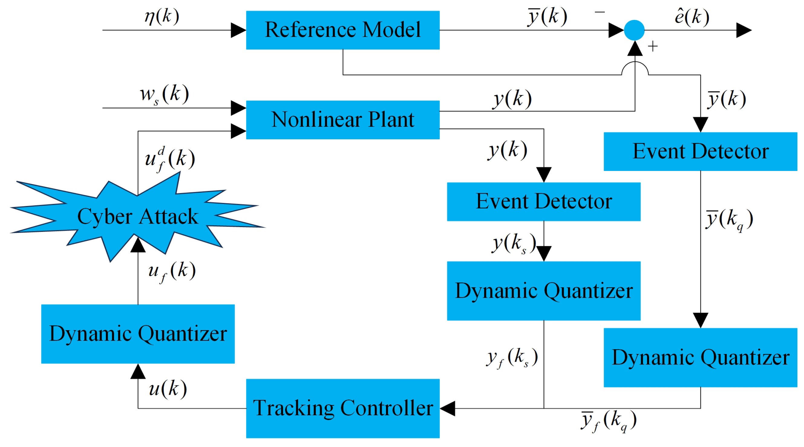
The dissipative output feedback tracking control problem has been considered for discrete-time nonlinear networked systems with dynamic quantization and stochastic deception attacks.

(2)

Both the event-triggered scheme and the dynamic quantization scheme with general online adjustment rule are introduced to decrease the data transmission amount and achieve the rational use of the limited communication and computation resources rather than only the event-triggered scheme or quantization scheme.

(3)

Based on the decoupling strategy, the corresponding design conditions of the desired static output feedback tracking controller are proposed in the form of linear matrix inequalities, rather than the specific design algorithm or the design conditions in terms of linear matrix inequality subject to restricted system matrices.

The remainder of this paper is organized as follows. In Section 2, the problem considered in this paper is presented. The main research findings of this paper are elaborated in Section 3, and the effectiveness of the proposed method is demonstrated through simulation examples in Section 4. The paper is summarized in Section 5.

2. Problem Formulation

Figure 1 gives the block diagram of the tracking control problem for nonlinear networked systems addressed in this paper. In the following, we will mathematically formulate the addressed problem.

2.1. T-S Fuzzy Systems

In this paper, the following discrete-time T-S fuzzy system will be utilized to approximate the concerned nonlinear plant and the $jth$ rule is expressed as follows:

$$\begin{array}{c}\mathrm{Plant}\mathrm{Rule}j:\mathrm{IF}{\vartheta }_1\left(k\right)\mathrm{is}{\Theta }_{j1},{\vartheta }_2\left(k\right)\mathrm{is}{\Theta }_{j2},\mathrm{and},\hfill \\ \dots ,\mathrm{and}{\vartheta }_{\theta }\left(k\right)\mathrm{is}{\Theta }_{j\theta }\hfill \end{array}$$

$$\begin{array}{c}\mathrm{THEN}x(k+1)=A_{j}x\left(k\right)+B_j{u}_f^d\left(k\right)+E_j{w}_s\left(k\right)\hfill \\ y\left(k\right)=C_{j}x\left(k\right)\hfill \end{array}$$

(1)

in which $j=1,2,\dots ,n$ and n represents the number of the if–then fuzzy rules. The fuzzy sets are denoted as ${\Theta }_{jm}$, with $m=1,2,\dots ,\theta$. $\vartheta \left(k\right)=[{\vartheta }_1\left(k\right),{\vartheta }_2\left(k\right),\dots ,{\vartheta }_{\theta }\left(k\right)]$ stands for the premise variable. $x\left(k\right)\in {\mathbb{R}}^{n_x}$, $u_f^d\left(k\right)\in {\mathbb{R}}^{n_u}$, and $y\left(k\right)\in {\mathbb{R}}^{n_y}$ are employed to indicate the state variable, the control input, and the measurement output, respectively. $w_s\left(k\right)\in {\mathbb{R}}^{n_{w_s}}$ is utilized to describe the disturbance input belonging to $l_2[0,\infty )$. $A_j\in {\mathbb{R}}^{n_x\times n_x}$, $B_j\in {\mathbb{R}}^{n_x\times n_u}$, $E_j\in {\mathbb{R}}^{n_x\times n_{w_s}}$, and $C_j\in {\mathbb{R}}^{n_y\times n_x}$ are used to represent the given system parameters. In addition, the fuzzy basis functions can be expressed as

$${\alpha }_j\left(\vartheta \left(k\right)\right)={\displaystyle \frac{{\prod }_{m=1}^{\theta }{\Theta }_{jm}\left({\vartheta }_m\left(k\right)\right)}{{\sum }_{j=1}^n{\prod }_{m=1}^{\theta }{\Theta }_{jm}\left({\vartheta }_m\left(k\right)\right)}}$$

(2)

where the grade of membership of ${\vartheta }_m\left(k\right)$ in ${\Theta }_{jm}$ is represented by ${\Theta }_{jm}\left({\vartheta }_m\left(k\right)\right)$. Then, one is able to conclude that

$${\alpha }_j\left(\vartheta \left(k\right)\right)\ge 0,\sum _{j=1}^n{\alpha }_j\left(\vartheta \left(k\right)\right),j=1,2,\dots ,n.$$

(3)

Moreover, one is able to infer the considered T-S fuzzy system (1) as

$$\begin{array}{c}x(k+1)=A\left(\alpha \right)x\left(k\right)+B\left(\alpha \right)u_f^d\left(k\right)+E\left(\alpha \right)w_s\left(k\right)\hfill \\ y\left(k\right)=C\left(\alpha \right)x\left(k\right)\hfill \end{array}$$

(4)

where

$$\begin{array}{c}A\left(\alpha \right)={\sum }_{j=1}^n{\alpha }_j\left(\vartheta \left(k\right)\right)A_j,B\left(\alpha \right)={\sum }_{j=1}^n{\alpha }_j\left(\vartheta \left(k\right)\right)B_j,\hfill \\ C\left(\alpha \right)={\sum }_{j=1}^n{\alpha }_j\left(\vartheta \left(k\right)\right)C_j,E\left(\alpha \right)={\sum }_{j=1}^n{\alpha }_j\left(\vartheta \left(k\right)\right)E_j.\hfill \end{array}$$

2.2. Reference Model

This paper is concerned with the output feedback tracking control problem and the reference model is presented as

$$\begin{array}{c}\overline{x}(k+1)=A_{\eta }\overline{x}\left(k\right)+B_{\eta }\eta \left(k\right)\hfill \\ \overline{y}\left(k\right)=C_{\eta }\overline{x}\left(k\right)\hfill \end{array}$$

(5)

where $\overline{x}\left(k\right)\in {\mathbb{R}}^{n_{\overline{x}}}$ indicates the state of the reference model, $\overline{y}\left(k\right)\in {\mathbb{R}}^{n_y}$ represents the measurement output of the reference model, $\eta \left(k\right)\in {\mathbb{R}}^{n_{\eta }}$ denotes the reference input, which is assumed to be energy-bounded. $A_{\eta }\in {\mathbb{R}}^{n_{\overline{x}}\times n_{\overline{x}}}$, $B_{\eta }\in {\mathbb{R}}^{n_{\overline{x}}\times n_{\eta }}$, and $C_{\eta }\in {\mathbb{R}}^{n_y\times n_{\overline{x}}}$ stand for known system matrices and $A_{\eta }$ is a Hurwitz matrix.

2.3. Event-Triggered Communication Scheme

The asynchronous event-triggered scheme developed in [38] will be employed in this paper to significantly decrease the data transmission amount and then conserve limited communication and computation resources. As in [38], the event-triggered condition associated with $y\left(k\right)$ is

$${\zeta }_y^T\left(k\right){\mathbf{N}}_1{\zeta }_y\left(k\right)\ge {\beta }_y{y}^T\left(k_s\right){\mathbf{N}}_{2}y\left(k_s\right)$$

(6)

in which ${\zeta }_y\left(k\right)=y\left(k\right)-y\left(k_s\right)$, with $y\left(k\right)$ and $y\left(k_s\right)$ denoting the measured output for the plant at the present instant and the one at the last triggering instant. ${\mathbf{N}}_1$ and ${\mathbf{N}}_2$ are two positive-definite weighting parameter matrices to be designed and $0\le {\beta }_y<1$ is the predetermined threshold.

The event-triggered condition associated with $\overline{y}\left(k\right)$ is

$${\zeta }_{\overline{y}}^T\left(k\right){\mathbf{M}}_1{\zeta }_{\overline{y}}\left(k\right)\ge {\beta }_{\overline{y}}{\overline{y}}^T\left(k_q\right){\mathbf{M}}_2\overline{y}\left(k_q\right)$$

(7)

in which ${\zeta }_{\overline{y}}\left(k\right)=\overline{y}\left(k\right)-\overline{y}\left(k_q\right)$, with $\overline{y}\left(k\right)$ and $\overline{y}\left(k_q\right)$ representing the measured output for the reference model at the present instant and the one at the last triggering instant. ${\mathbf{M}}_1$ and ${\mathbf{M}}_2$ indicate two positive-definite weighting parameter matrices to be designed and $0\le {\beta }_{\overline{y}}<1$ is the predetermined threshold.

Remark 1.

If we select ${\beta }_y={\beta }_{\overline{y}}=0$, the asynchronous event-triggered scheme investigated herein will be reduced to the traditional time-triggered scheme employed in [30,33]. If we select ${\mathbf{N}}_1={\mathbf{N}}_2$ and ${\mathbf{M}}_1={\mathbf{M}}_2$, the asynchronous event-triggered scheme employed herein will be reduced to the one developed in [37]. Moreover, as claimed in [30,37,38], based on the fact that the various parts of the system are usually located at the different places for the tracking problem of networked systems, it can be concluded that the asynchronous event-triggered scheme utilized herein is more general than the synchronous event-triggered scheme considered in [23,35,36].

2.4. Dynamic Quantizers

As is well known, quantization is also considered to be an effective strategy to significantly decrease the data transmission amount and then achieve the rational use of the limited communication and computation resources. As far as the existing literature, there are mainly two schemes for investigating networked systems with quantization, i.e., the dynamic quantization scheme and the static quantization scheme. This paper adopts the dynamic quantization scheme proposed in [3]. Based on the results in [3], it can be obtained that

$$|f_{\varsigma }\left(\varsigma \right)-\varsigma |\le {\Delta }_{\varsigma },\mathrm{IF}\left|\varsigma \right|\le {\mathbb{M}}_{\varsigma }$$

(8)

$$|f_{\varsigma }\left(\varsigma \right)-\varsigma |>{\mathbb{M}}_{\varsigma }-{\Delta }_{\varsigma },\mathrm{IF}\left|\varsigma \right|>{\mathbb{M}}_{\varsigma }$$

(9)

where ${\mathbb{M}}_{\varsigma }$ represents the range of the quantizer and ${\Delta }_{\varsigma }$ represents the bound on the quantization error.

According to [3], one is able to deduce that the measured outputs with quantization and the control input with quantization considered in this paper are

$$y_f\left(k\right)=f_{{\rho }_y}\left(y\left(k_s\right)\right)={\rho }_y{f}_y\left({\displaystyle \frac{y\left(k_s\right)}{{\rho }_y}}\right)=l_y\left(k_s\right)+y\left(k_s\right)$$

(10)

$${\overline{y}}_f\left(k\right)=f_{{\rho }_{\overline{y}}}\left(\overline{y}\left(k_q\right)\right)={\rho }_{\overline{y}}{f}_{\overline{y}}\left({\displaystyle \frac{\overline{y}\left(k_q\right)}{{\rho }_{\overline{y}}}}\right)=l_{\overline{y}}\left(k_q\right)+\overline{y}\left(k_q\right)$$

(11)

$$u_f\left(k\right)=f_{{\rho }_u}\left(u\left(k\right)\right)={\rho }_u{f}_u\left({\displaystyle \frac{u\left(k\right)}{{\rho }_u}}\right)=l_u\left(k\right)+u\left(k\right)$$

(12)

where ${\rho }_{\varsigma }$ ($\varsigma =y,\overline{y},u$) are used to represent the dynamic parameters of the quantizer $f_{\varsigma }\left(\varsigma \right)$ and

$$\begin{array}{c}{l}_y\left(k_s\right)={\rho }_y\left(f_y\left({\displaystyle \frac{y\left(k_s\right)}{{\rho }_y}}\right)-{\displaystyle \frac{y\left(k_s\right)}{{\rho }_y}}\right),\hfill \\ l_{\overline{y}}\left(k_q\right)={\rho }_{\overline{y}}\left(f_{\overline{y}}\left({\displaystyle \frac{\overline{y}\left(k_q\right)}{{\rho }_{\overline{y}}}}\right)-{\displaystyle \frac{\overline{y}\left(k_q\right)}{{\rho }_{\overline{y}}}}\right),\hfill \\ l_u\left(k\right)={\rho }_u\left(f_u\left({\displaystyle \frac{u\left(k\right)}{{\rho }_u}}\right)-{\displaystyle \frac{u\left(k\right)}{{\rho }_u}}\right).\hfill \end{array}$$

Remark 2.

In contrast to the static quantization scheme utilized in [33,37], the main advantage of the dynamic quantization scheme introduced herein is that the asymptotic stability is able to be ensured under the finite number of quantization levels. The main reason for the above phenomenon is that the quantization levels can be scaled dynamically in order to increase the region of attraction and to attenuate the steady-state limit cycle. Compared with the existing investigations on quantized tracking control that focus solely on quantized input [25] or multiple quantized outputs [39], this paper presents a more generalized quantized tracking control framework by incorporating three dynamic quantizers. The proposed method significantly improves the efficient utilization of limited communication and computational resources.

2.5. Deception Attacks

As is well known, due to the openness and unreliability of the communication networks, cyber attacks are unavoidable during the process of signal transmission in networked systems. As a result, the effect of stochastic deception attacks on quantized control input will be addressed in this paper. Additionally, one is able to formulate the quantized control input subject to stochastic deception attacks as

$$\begin{array}{c}{u}_f^d\left(k\right)=\chi \left(k\right)d_u\left(k\right)+(1-\chi \left(k\right))u_f\left(k\right)\hfill \end{array}$$

(13)

Here, $d_u\left(k\right)$ denotes the the deception signal and $\chi \left(k\right)$ stands for a Bernoulli distributed white sequence which is satisfied with the following two conditions:

$$\begin{array}{c}\mathrm{Prob}\{\chi \left(k\right)=1\}=\mathbf{E}\left\{\chi \left(k\right)\right\}=\overline{\chi }\hfill \\ \mathrm{Prob}\{\chi \left(k\right)=0\}=1-\overline{\chi }.\hfill \end{array}$$

(14)

$\chi \left(k\right)=1$ signifies that the received signal is the deception signal (that is, $u_f^d\left(k\right)=d_u\left(k\right)$) and $\chi \left(k\right)=0$ means that the received signal is the quantized control input (that is, $u_f^d\left(k\right)=u_f\left(k\right)$). Moreover, as in [39], a natural assumption with regard to the deception signal is given as follows:

$$d_u^T\left(k\right)d_u\left(k\right)\le u_f^T\left(k\right)D_u^T{D}_u{u}_f\left(k\right)$$

(15)

where $D_u$ is the known matrix for $d_u\left(k\right)$.

2.6. Tracking Controller and Resulting System

For the discussed tracking control problem herein, the static output feedback tracking controller with the following form will be employed:

$$u\left(k\right)=L_y{y}_f\left(k\right)+L_{\overline{y}}{\overline{y}}_f\left(k\right)$$

(16)

in which $L_y\in {\mathbb{R}}^{n_u\times n_y}$ and $L_{\overline{y}}\in {\mathbb{R}}^{n_u\times n_y}$ are controller parameters to be determined.

Then, the resulting system is able to be expressed as

$$\begin{array}{c}\widehat{x}(k+1)=({\mathbb{A}}_1+\tilde{\chi }\left(k\right){\mathbb{A}}_2)\psi \left(k\right)+({\mathbb{D}}_1+\tilde{\chi }\left(k\right){\mathbb{D}}_2)d_u\left(k\right)\hfill \\ +({\mathbb{L}}_1+\tilde{\chi }\left(k\right){\mathbb{L}}_2)l_y\left(k_s\right)+({\mathbb{L}}_3+\tilde{\chi }\left(k\right){\mathbb{L}}_4)l_{\overline{y}}\left(k_q\right)\hfill \\ +({\mathbb{L}}_5+\tilde{\chi }\left(k\right){\mathbb{L}}_6)l_u\left(k\right)+{\mathbb{E}}_{1}w\left(k\right)\hfill \\ \widehat{e}\left(k\right)=\mathbb{C}\psi \left(k\right)\hfill \end{array}$$

(17)

where ${\widehat{x}}^T\left(k\right)=\left[x^T\left(k\right){\overline{x}}^T\left(k\right)\right]$, $w^T\left(k\right)=\left[w_s^T\left(k\right){\eta }^T\left(k\right)\right]$, ${\psi }^T\left(k\right)=\left[x^T\left(k\right){\overline{x}}^T\left(k\right){\zeta }_y^T\left(k\right){\zeta }_{\overline{y}}^T\left(k\right)\right]$, $\widehat{e}\left(k\right)=y\left(k\right)-\overline{y}\left(k\right)$, $\tilde{\chi }\left(k\right)=\chi \left(k\right)-\overline{\chi }$, and

$$\begin{array}{c}{\mathbb{A}}_1=\left[\begin{array}{cccc}{\Gamma }_1& {\Gamma }_2& {\Gamma }_3& {\Gamma }_4\\ 0& A_{\eta }& 0& 0\end{array}\right],{\mathbb{D}}_1=\left[\begin{array}{c}\overline{\chi }B\left(\alpha \right)\\ 0\end{array}\right],\hfill \\ {\mathbb{A}}_2=\left[\begin{array}{cccc}{\Gamma }_5& {\Gamma }_6& {\Gamma }_7& {\Gamma }_8\\ 0& 0& 0& 0\end{array}\right],{\mathbb{D}}_2=\left[\begin{array}{c}B\left(\alpha \right)\\ 0\end{array}\right],\hfill \\ {\mathbb{L}}_1=\left[\begin{array}{c}(1-\overline{\chi })B\left(\alpha \right)L_y\\ 0\end{array}\right],{\mathbb{L}}_2=\left[\begin{array}{c}-B\left(\alpha \right)L_y\\ 0\end{array}\right],\hfill \\ {\mathbb{L}}_3=\left[\begin{array}{c}(1-\overline{\chi })B\left(\alpha \right)L_{\overline{y}}\\ 0\end{array}\right],{\mathbb{L}}_4=\left[\begin{array}{c}-B\left(\alpha \right)L_{\overline{y}}\\ 0\end{array}\right],\hfill \\ {\mathbb{L}}_5=\left[\begin{array}{c}(1-\overline{\chi })B\left(\alpha \right)\\ 0\end{array}\right],{\mathbb{L}}_6=\left[\begin{array}{c}-B\left(\alpha \right)\\ 0\end{array}\right],\hfill \\ {\mathbb{E}}_1=\left[\begin{array}{cc}E\left(\alpha \right)& 0\\ 0& B_{\eta }\end{array}\right],\mathbb{C}=[C\left(\alpha \right)-C_{\eta }00],\hfill \end{array}$$

${\Gamma }_1=A\left(\alpha \right)+(1-\overline{\chi })B\left(\alpha \right)L_{y}C\left(\alpha \right)$, ${\Gamma }_2=(1-\overline{\chi })B\left(\alpha \right)L_{\overline{y}}{C}_{\eta }$, ${\Gamma }_3=-(1-\overline{\chi })B\left(\alpha \right)L_y$, ${\Gamma }_4=-(1-\overline{\chi })B\left(\alpha \right)L_{\overline{y}}$, ${\Gamma }_5=-B\left(\alpha \right)L_{y}C\left(\alpha \right)$, ${\Gamma }_6=-B\left(\alpha \right)L_{\overline{y}}{C}_{\eta }$, ${\Gamma }_7=B\left(\alpha \right)L_y$, ${\Gamma }_8=B\left(\alpha \right)L_{\overline{y}}$.

Before introducing the discussed tracking control problem, we first present the following definitions with regard to the stochastic stability and the dissipative tracking performance, which is essential to deal with the analysis problem of the resulting system in (17).

Definition 1.

For zero initial condition $\widehat{x}\left(0\right)=0$, the stochastic stability of the resulting system in (17) can be ensured when $w\left(k\right)=0$, if there exists a matrix $\mathbb{P}>0$ satisfying

$$\begin{array}{c}\mathbf{E}\left\{{\displaystyle \sum _{k=0}^{\infty }}{\left|\widehat{x}\left(k\right)\right|}^2|\widehat{x}\left(0\right)\right\}<{\widehat{x}}^T\left(0\right)\mathbb{P}\widehat{x}\left(0\right).\hfill \end{array}$$

(18)

Definition 2.

Suppose that the matrices $J_1=J_1^T\in {\mathbb{R}}^{n_y\times n_y}\le 0$, $J_2\in {\mathbb{R}}^{n_y\times (n_{w_s}+n_{\eta })}$, $J_3=J_3^T\in {\mathbb{R}}^{(n_{w_s}+n_{\eta })\times (n_{w_s}+n_{\eta })}$, and $-J_1=J_{11}^T{J}_{11}$ with $J_{11}\in {\mathbb{R}}^{n_y\times n_y}\ge 0$ are known. Then, in the presence of zero initial condition $(\widehat{x}\left(0\right)=0)$, the given dissipative tracking performance γ of the resulting system in (17) can be ensured as long as the inequality

$$\begin{array}{c}{\sum }_{k=0}^{\mathfrak{r}}\left({\widehat{e}}^T\left(k\right)J_1\widehat{e}\left(k\right)+{\widehat{e}}^T\left(k\right)J_{2}w\left(k\right)+w^T\left(k\right)\right.\hfill \\ \left.\times J_2^T\widehat{e}\left(k\right)+w^T\left(k\right)(J_3-\gamma I)w\left(k\right)\right)\ge 0\hfill \end{array}$$

(19)

is satisfied for $\mathfrak{r}>0$.

Remark 3.

If we select $J_1=-I$, $J_2=0$, $J_3=({\gamma }^2+\gamma I)$, the dissipative tracking performance given in Definition 1 will be reduced to the ${\mathcal{H}}_{\infty }$ tracking performance investigated in [22,23,27,28,29,30,31,32]. If we select $J_1=0$, $J_2=I$, $J_3=2\gamma I$, the dissipative tracking performance given in Definition 1 will be reduced to the passive tracking performance [40]. Furthermore, if we select $J_1=-\wp I$, $J_2=(1-\wp )I$, $J_3=(\wp ({\gamma }^2-\gamma )+2\gamma )I$ with $0\le \wp \le 1$ standing for a given weighting parameter, the dissipative tracking performance given in Definition 1 will be reduced to the mixed passive/${\mathcal{H}}_{\infty }$ performance. Therefore, it is able to be concluded that the dissipative tracking problem considered herein is more general than the ${\mathcal{H}}_{\infty }$ tracking problem addressed in [22,23,27,28,29,30,31,32].

The investigated event-based tracking control problem in this paper is to design the static output feedback tracking controller in (16) such that the resulting system in (17) is satisfied with the following two requirements.

(1)

The stochastic stability of the resulting system in (17) is guaranteed for $w\left(k\right)=0$.

(2)

The given dissipative tracking performance of the resulting system in (17) is guaranteed for the zero initial condition.

In addition, to deal with the tracking controller design problem, a momentous lemma will be introduced, which is presented as follows.

Lemma 1

([14]). For matrices ${\pounds }_{\mathsf{ı}}(\mathsf{ı}=1,2,3,4)$ with appropriate dimensions, the inequality ${\pounds }_1+{\pounds }_2{\pounds }_3+{\pounds }_3^T{\pounds }_2^T<0$ is satisfied, if there exists a matrix ${\pounds }_4$ such that

$$\left[\begin{array}{cc}{\pounds }_1& \ast \\ {\pounds }_2^T+{\pounds }_4{\pounds }_3& -{\pounds }_4-{\pounds }_4^T\end{array}\right]<0.$$

(20)

3. Main Results

3.1. Dissipative Tracking Performance Analysis

In this part, the analysis problem for the dissipative tracking performance of the resulting system in (17) will be studied. More specifically, based on the premise that the parameters for the desired tracking controller in (16) are provided, according to the Lyapunov theory, we shall formulate a sufficient condition in the following theorem to guarantee the stochastic stability in the sense of Definition 1 together with the dissipative tracking performance in the sense of Definition 2 of the resulting system in (17).

Theorem 1.

For given the quantization ranges ${\mathbb{M}}_{\varsigma }$, the quantization error bounds ${\Delta }_{\varsigma }$, the constants $0<a_{1\varsigma }<a_{2\varsigma }$, $0<b_{1\varsigma }<b_{2\varsigma }$, satisfying $a_{1\varsigma }{b}_{1\varsigma }>1$ for $\varsigma =y,\overline{y},u$, and the constants $0\le {\beta }_y<1$, $0\le {\beta }_{\overline{y}}<1$. The stochastic stability as well as the prescribed dissipative tracking performance of the resulting system in (17) will be guaranteed if there exist matrices $P>0$, ${\mathbf{N}}_1>0$, ${\mathbf{N}}_2>0$, ${\mathbf{M}}_1>0$, and ${\mathbf{M}}_2>0$, positive scalars ${\delta }_y$, ${\delta }_{\overline{y}}$, and $o_{\varsigma }$, $\varsigma =y,\overline{y},u$ satisfying the following inequalities:

$${\displaystyle \frac{a_{1\varsigma }}{{\mathbb{M}}_{\varsigma }}}\le o_{\varsigma }\le {\displaystyle \frac{a_{2\varsigma }}{{\mathbb{M}}_{\varsigma }}},\varsigma =y,\overline{y},u$$

(21)

$$\left[\begin{array}{cc}{\prod }_{11}& \ast \\ {\prod }_{21}& {\prod }_{22}\end{array}\right]<0$$

(22)

$$L_y^T{L}_y<{\displaystyle \frac{1}{{\delta }_y}}I$$

(23)

$$L_{\overline{y}}^T{L}_{\overline{y}}<{\displaystyle \frac{1}{{\delta }_{\overline{y}}}}I$$

(24)

where

$$\begin{array}{c}{\prod }_{11}=-\left[\begin{array}{cccccc}\mathfrak{P}& \ast & \ast & \ast & \ast & \ast \\ 0& I& \ast & \ast & \ast & \ast \\ 0& 0& I& \ast & \ast & \ast \\ 0& 0& 0& I& \ast & \ast \\ 0& 0& 0& 0& I& \ast \\ J_2^T\mathbb{C}& 0& 0& 0& 0& J_3-\gamma I\end{array}\right],\hfill \\ {\prod }_{21}={\left[S_0^T{S}_1^T{S}_2^T{S}_3^T{S}_4^T{S}_5^T{S}_6^T\right]}^T,\hfill \\ {\prod }_{22}=-diag\{P^{-1},P^{-1},I,I,I,{\delta }_{y}I,{\delta }_{\overline{y}}I\},\hfill \end{array}$$

$\mathfrak{P}=\widehat{P}-{\beta }_y{\Lambda }_y^T{\mathbf{N}}_2{\Lambda }_y-{\beta }_{\overline{y}}{\Lambda }_{\overline{y}}^T{\mathbf{M}}_2{\Lambda }_{\overline{y}}+{\mathbb{C}}^T{J}_1\mathbb{C}+\overline{N}+\overline{M}$, $S_0=\left[{\mathbb{A}}_1{\mathbb{D}}_1{\mathbb{L}}_1{\mathbb{L}}_3{\mathbb{L}}_5{\mathbb{E}}_1\right]$, $S_1=\left[\widehat{\chi }{\mathbb{A}}_2\widehat{\chi }{\mathbb{D}}_2\widehat{\chi }{\mathbb{L}}_2\widehat{\chi }{\mathbb{L}}_4\widehat{\chi }{\mathbb{L}}_{6}0\right]$, $S_2=\left[{\tilde{D}}_{u}0D_u{L}_y{D}_u{L}_{\overline{y}}{D}_{u}0\right]$, $S_3=\left[{\sigma }_y{\Lambda }_{y}00000\right]$, $S_4=\left[{\sigma }_{\overline{y}}{\Lambda }_{\overline{y}}00000\right]$, $S_5=\left[\sqrt{2}(1+{\sigma }_y){\sigma }_u{\Lambda }_{y}00000\right]$, $S_6=\left[\sqrt{2}(1+{\sigma }_{\overline{y}}){\sigma }_u{\Lambda }_{\overline{y}}00000\right]$, $\widehat{P}=diag\{P,0,0\}$, ${\Lambda }_y=[C\left(\alpha \right)0-I0]$, ${\Lambda }_{\overline{y}}=[0C_{\eta }0-I]$, $\overline{N}=diag\{0,0,{\mathbf{N}}_1,0\}$, $\overline{M}=diag\{0,0,0,{\mathbf{M}}_1\}$, ${\tilde{D}}_u=[D_u{L}_{y}C\left(\alpha \right)D_u{L}_{\overline{y}}{C}_{\eta }-D_u{L}_y-D_u{L}_{\overline{y}}]$, ${\sigma }_y={\displaystyle \frac{a_{2y}{b}_{2y}{\Delta }_y}{{\mathbb{M}}_y}}$, ${\sigma }_{\overline{y}}={\displaystyle \frac{a_{2\overline{y}}{b}_{2\overline{y}}{\Delta }_{\overline{y}}}{{\mathbb{M}}_{\overline{y}}}}$, ${\sigma }_u={\displaystyle \frac{a_{2u}{b}_{2u}{\Delta }_u}{{\mathbb{M}}_u}}$, and it is able to formulate the online adjusting scheme of the dynamic parameters ${\rho }_{\varsigma }$, $\varsigma =y,\overline{y},u$ as

$$\begin{array}{c}{b}_{1y}{o}_y|y\left(k_s\right)|\le {\rho }_y\le b_{2y}{o}_y\left|y\left(k_s\right)\right|\hfill \\ b_{1\overline{y}}{o}_{\overline{y}}|\overline{y}\left(k_q\right)|\le {\rho }_{\overline{y}}\le b_{2\overline{y}}{o}_{\overline{y}}\left|\overline{y}\left(k_q\right)\right|\hfill \\ b_{1u}{o}_u|\overline{u}\left(k\right)|\le {\rho }_u\le b_{2u}{o}_u\left|\overline{u}\left(k\right)\right|.\hfill \end{array}$$

(25)

Proof. 

For the resulting system (17), one can naturally formulate the Lyapunov function as

$$V\left(\widehat{x}\left(k\right)\right)={\widehat{x}}^T\left(k\right)P\widehat{x}\left(k\right),P>0.$$

(26)

In consideration of the fact that $\mathbf{E}\left\{{\tilde{\chi }}^2\left(k\right)\right\}=\overline{\chi }\left(1-\overline{\chi }\right)={\widehat{\chi }}^2$, we have

$$\begin{array}{c}\mathbf{E}\left\{V\left(\widehat{x}(k+1)\right)\right\}-V\left(\widehat{x}\left(k\right)\right)-{\widehat{e}}^T\left(k\right)J_1\widehat{e}\left(k\right)-{\widehat{e}}^T\left(k\right)\hfill \\ \times J_{2}w\left(k\right)-w^T\left(k\right)J_2^T\widehat{e}\left(k\right)-w^T\left(k\right)(J_3-\gamma I)w\left(k\right)\hfill \\ =\mathbf{E}\left\{{\widehat{x}}^T(k+1)P\widehat{x}(k+1)\right\}-{\widehat{x}}^T\left(k\right)P\widehat{x}\left(k\right)-{\widehat{e}}^T\left(k\right)\hfill \\ \times J_1\widehat{e}\left(k\right)-{\widehat{e}}^T\left(k\right)J_{2}w\left(k\right)-w^T\left(k\right)J_2^T\widehat{e}\left(k\right)\hfill \\ -w^T\left(k\right)(J_3-\gamma I)w\left(k\right)\hfill \\ =\mathbf{E}\left\{(({\mathbb{A}}_1+\tilde{\chi }\left(k\right){\mathbb{A}}_2)\psi \left(k\right)+({\mathbb{D}}_1+\tilde{\chi }\left(k\right){\mathbb{D}}_2)d_u\left(k\right)\right.\hfill \\ +({\mathbb{L}}_1+\tilde{\chi }\left(k\right){\mathbb{L}}_2)l_y\left(k_s\right)+({\mathbb{L}}_3+\tilde{\chi }\left(k\right){\mathbb{L}}_4)l_{\overline{y}}\left(k_q\right)\hfill \\ +({\mathbb{L}}_5+\tilde{\chi }\left(k\right){\mathbb{L}}_6)l_u\left(k\right)+{\mathbb{E}}_1{w\left(k\right))}^{T}P\hfill \\ \times (({\mathbb{A}}_1+\tilde{\chi }\left(k\right){\mathbb{A}}_2)\psi \left(k\right)+({\mathbb{D}}_1+\tilde{\chi }\left(k\right){\mathbb{D}}_2)d_u\left(k\right)\hfill \\ +({\mathbb{L}}_1+\tilde{\chi }\left(k\right){\mathbb{L}}_2)l_y\left(k_s\right)+({\mathbb{L}}_3+\tilde{\chi }\left(k\right){\mathbb{L}}_4)l_{\overline{y}}\left(k_q\right)\hfill \\ \left.+({\mathbb{L}}_5+\tilde{\chi }\left(k\right){\mathbb{L}}_6)l_u\left(k\right)+{\mathbb{E}}_{1}w\left(k\right))\right\}\hfill \\ -{\widehat{x}}^T\left(k\right)P\widehat{x}\left(k\right)-{\psi }^T\left(k\right){\mathbb{C}}^T{J}_1\mathbb{C}\psi \left(k\right)-{\psi }^T\left(k\right)\hfill \\ \times {\mathbb{C}}^T{J}_{2}w\left(k\right)-w^T\left(k\right)J_2^T\mathbb{C}\psi \left(k\right)\hfill \\ -w^T\left(k\right)(J_3-\gamma I)w\left(k\right)\hfill \\ ={\Psi }^T\left(k\right)(\mathbf{E}\left\{(\left[{\mathbb{A}}_1{\mathbb{D}}_1{\mathbb{L}}_1{\mathbb{L}}_3{\mathbb{L}}_5{\mathbb{E}}_1\right]\right.\hfill \\ +\tilde{\chi }\left(k\right)\left[{\mathbb{A}}_2{\mathbb{D}}_2{\mathbb{L}}_2{\mathbb{L}}_4{\mathbb{L}}_{6}0\right]{)}^{T}P\hfill \\ \times (\left[{\mathbb{A}}_1{\mathbb{D}}_1{\mathbb{L}}_1{\mathbb{L}}_3{\mathbb{L}}_5{\mathbb{E}}_1\right]\hfill \\ \left.+\tilde{\chi }\left(k\right)\left[{\mathbb{A}}_2{\mathbb{D}}_2{\mathbb{L}}_2{\mathbb{L}}_4{\mathbb{L}}_{6}0\right])\right\}\hfill \\ -{\left[\mathbb{C}00000\right]}^T{J}_1\left[\mathbb{C}00000\right]\hfill \\ -{\left[\mathbb{C}00000\right]}^T\left[00000J_2\right]\hfill \\ -{\left[00000J_2\right]}^T\left[\mathbb{C}00000\right]\hfill \\ -diag\{\widehat{P},0,0,0,0,J_3-\gamma I\})\Psi \left(k\right)\hfill \\ ={\Psi }^T\left(k\right)Z_0\Psi \left(k\right)\hfill \end{array}$$

(27)

where ${\Psi }^T\left(k\right)=\left[{\psi }^T\left(k\right)d_u^T\left(k\right)l_y^T\left(k_s\right)l_{\overline{y}}^T\left(k_q\right)l_u^T\left(k\right)w^T\left(k\right)\right]$ and

$$\begin{array}{c}{Z}_0={\left[{\mathbb{A}}_1{\mathbb{D}}_1{\mathbb{L}}_1{\mathbb{L}}_3{\mathbb{L}}_5{\mathbb{E}}_1\right]}^{T}P\left[{\mathbb{A}}_1{\mathbb{D}}_1{\mathbb{L}}_1{\mathbb{L}}_3{\mathbb{L}}_5{\mathbb{E}}_1\right]\hfill \\ +{\widehat{\chi }}^2{\left[{\mathbb{A}}_2{\mathbb{D}}_2{\mathbb{L}}_2{\mathbb{L}}_4{\mathbb{L}}_{6}0\right]}^{T}P\left[{\mathbb{A}}_2{\mathbb{D}}_2{\mathbb{L}}_2{\mathbb{L}}_4{\mathbb{L}}_{6}0\right]\hfill \\ -{\left[\mathbb{C}00000\right]}^T{J}_1\left[\mathbb{C}00000\right]\hfill \\ -{\left[\mathbb{C}00000\right]}^T\left[00000J_2\right]\hfill \\ -{\left[00000J_2\right]}^T\left[\mathbb{C}00000\right]\hfill \\ -diag\{\widehat{P},0,0,0,0,J_3-\gamma I\}.\hfill \end{array}$$

In light of the inequalities presented in (6) and (7), it is possible to deduce that ${\beta }_y{(y\left(k\right)-{\zeta }_y\left(k\right))}^T{\mathbf{N}}_2(y\left(k\right)-{\zeta }_y\left(k\right))-{\zeta }_y^T\left(k\right){\mathbf{N}}_1{\zeta }_y\left(k\right)\ge 0$ and ${\beta }_{\overline{y}}{(\overline{y}\left(k\right)-{\zeta }_{\overline{y}}\left(k\right))}^T{\mathbf{M}}_2(\overline{y}\left(k\right)-{\zeta }_{\overline{y}}\left(k\right))-{\zeta }_{\overline{y}}^T\left(k\right){\mathbf{M}}_1{\zeta }_{\overline{y}}\left(k\right)\ge 0$; that is,

$${\Psi }^T\left(k\right)Z_1\Psi \left(k\right)\ge 0$$

(28)

$${\Psi }^T\left(k\right)Z_2\Psi \left(k\right)\ge 0$$

(29)

where

$$\begin{array}{c}{Z}_1={\beta }_y{\left[{\Lambda }_{y}00000\right]}^T{\mathbf{N}}_2\left[{\Lambda }_{y}00000\right]\hfill \\ -diag\{\overline{N},0,0,0,0,0\},\hfill \\ Z_2={\beta }_{\overline{y}}{\left[{\Lambda }_{\overline{y}}00000\right]}^T{\mathbf{M}}_2\left[{\Lambda }_{\overline{y}}00000\right]\hfill \\ -diag\{\overline{M},0,0,0,0,0\}.\hfill \end{array}$$

From the constraint in (21) combined with the online adjusting scheme in (25), we are able to deduce that $\left|y\left(k_s\right)\right|\le {\displaystyle \frac{{\mathbb{M}}_y}{a_{1y}{b}_{1y}}}{\rho }_y\le {\rho }_y{\mathbb{M}}_y$. Moreover, based on the constraint in (8), we have $l_y\left(k_s\right)\le {\rho }_y{\Delta }_y\le b_{2y}{o}_y{\Delta }_y\left|y\left(k_s\right)\right|\le {\sigma }_y\left|y\left(k_s\right)\right|$, i.e., $l_y^T\left(k_s\right)l_y\left(k_s\right)\le {\sigma }_y^2{(y\left(k\right)-{\zeta }_y\left(k\right))}^T(y\left(k\right)-{\zeta }_y\left(k\right))$, which can be denoted as

$${\Psi }^T\left(k\right)Z_3\Psi \left(k\right)\ge 0$$

(30)

with

$$\begin{array}{c}{Z}_3={\left[{\sigma }_y{\Lambda }_{y}00000\right]}^T\left[{\sigma }_y{\Lambda }_{y}00000\right]\hfill \\ -diag\{0,0,I,0,0,0\}.\hfill \end{array}$$

Similarly, combining the inequality in (21), the online adjusting scheme in (25), and the constraint in (8), we can obtain that $l_{\overline{y}}^T\left(k_q\right)l_{\overline{y}}\left(k_q\right)\le {\sigma }_{\overline{y}}^2{(\overline{y}\left(k\right)-{\zeta }_{\overline{y}}\left(k\right))}^T(\overline{y}\left(k\right)-{\zeta }_{\overline{y}}\left(k\right))$, which can be expressed as

$${\Psi }^T\left(k\right)Z_4\Psi \left(k\right)\ge 0$$

(31)

with

$$\begin{array}{c}{Z}_4={\left[{\sigma }_{\overline{y}}{\Lambda }_{\overline{y}}00000\right]}^T\left[{\sigma }_{\overline{y}}{\Lambda }_{\overline{y}}00000\right]\hfill \\ -diag\{0,0,0,I,0,0\}.\hfill \end{array}$$

In addition, for the quantized control input, we are able to deduce that $l_u^T\left(k\right)l_u\left(k\right)\le {\sigma }_u^2{u}^T\left(k\right)u\left(k\right)$; that is,

$$\begin{array}{c}{l}_u^T\left(k\right)l_u\left(k\right)\hfill \\ \le {\sigma }_u^2{(L_y{y}_f\left(k\right)+L_{\overline{y}}{\overline{y}}_f\left(k\right))}^T(L_y{y}_f\left(k\right)+L_{\overline{y}}{\overline{y}}_f\left(k\right))\hfill \\ ={\sigma }_u^2(y_f^T\left(k\right)L_y^T{L}_y{y}_f\left(k\right)+y_f^T\left(k\right)L_y^T{L}_{\overline{y}}{\overline{y}}_f\left(k\right)\hfill \\ +{\overline{y}}_f^T\left(k\right)L_{\overline{y}}^T{L}_y{y}_f\left(k\right)+{\overline{y}}_f^T\left(k\right)L_{\overline{y}}^T{L}_{\overline{y}}{\overline{y}}_f\left(k\right))\hfill \\ \le {\sigma }_u^2(2y_f^T\left(k\right)L_y^T{L}_y{y}_f\left(k\right)+2{\overline{y}}_f^T\left(k\right)L_{\overline{y}}^T{L}_{\overline{y}}{\overline{y}}_f\left(k\right))\hfill \\ \le 2{\sigma }_u^2({\displaystyle \frac{1}{{\delta }_y}}{y}_f^T\left(k\right)y_f\left(k\right)+{\displaystyle \frac{1}{{\delta }_{\overline{y}}}}{\overline{y}}_f^T\left(k\right){\overline{y}}_f\left(k\right))\hfill \end{array}$$

(32)

In consideration of the measured output with quantization presented in (10), we are able to conclude that

$$\begin{array}{c}\left|y_f\left(k\right)\right|=\left|l_y\left(k_s\right)+y\left(k_s\right)\right|\hfill \\ \le \left|l_y\left(k_s\right)\right|+\left|y\left(k_s\right)\right|\hfill \\ \le {\sigma }_y\left|y\left(k_s\right)\right|+\left|y\left(k_s\right)\right|\hfill \\ =(1+{\sigma }_y)\left|y\left(k_s\right)\right|\hfill \end{array}$$

(33)

which can be represented as

$$y_f^T\left(k\right)y_f\left(k\right)\le {(1+{\sigma }_y)}^2{y}^T\left(k_s\right)y\left(k_s\right)$$

(34)

Similarly, for ${\overline{y}}_f\left(k\right)$, we obtain $\left|{\overline{y}}_f\left(k\right)\right|\le (1+{\sigma }_{\overline{y}})\left|\overline{y}\left(k_q\right)\right|$, which can be rewritten as

$$\begin{array}{c}{\overline{y}}_f^T\left(k\right){\overline{y}}_f\left(k\right)\le {(1+{\sigma }_{\overline{y}})}^2{\overline{y}}^T\left(k_q\right)\overline{y}\left(k_q\right)\hfill \end{array}$$

(35)

By considering the inequalities in (34) and (35), one is able to reformulate the condition obtained in (32) as

$$\begin{array}{c}{l}_u^T\left(k\right)l_u\left(k\right)\le 2{\sigma }_u^2\left({\displaystyle \frac{1}{{\delta }_y}}{(1+{\sigma }_y)}^2{y}^T\left(k_s\right)y\left(k_s\right)\right.\hfill \\ \left.+{\displaystyle \frac{1}{{\delta }_{\overline{y}}}}{(1+{\sigma }_{\overline{y}})}^2{\overline{y}}^T\left(k_q\right)\overline{y}\left(k_q\right)\right)\hfill \end{array}$$

(36)

which is equivalent to

$${\Psi }^T\left(k\right)Z_5\Psi \left(k\right)\ge 0$$

(37)

with

$$\begin{array}{c}{Z}_5={\displaystyle \frac{2{(1+{\sigma }_y)}^2}{{\delta }_y}}{\left[{\sigma }_u{\Lambda }_{y}00000\right]}^T\left[{\sigma }_u{\Lambda }_{y}00000\right]\hfill \\ +{\displaystyle \frac{2{(1+{\sigma }_{\overline{y}})}^2}{{\delta }_{\overline{y}}}}{\left[{\sigma }_u{\Lambda }_{\overline{y}}00000\right]}^T\left[{\sigma }_u{\Lambda }_{\overline{y}}00000\right]\hfill \\ -diag\{0,0,0,0,I,0\}.\hfill \end{array}$$

Afterwards, by recalling the constraint on the deception signal in (15), we have

$${\Psi }^T\left(k\right)Z_6\Psi \left(k\right)\ge 0$$

(38)

where

$$\begin{array}{c}{Z}_6={\left[{\tilde{D}}_{u}0{\widehat{D}}_u{D}_u{L}_{\overline{y}}{D}_{u}0\right]}^T\left[{\tilde{D}}_{u}0{\widehat{D}}_u{D}_u{L}_{\overline{y}}{D}_{u}0\right]\hfill \\ -diag\{0,I,0,0,0,0\}\hfill \end{array}$$

with ${\widehat{D}}_u=D_u{L}_y$.

According to the Schur complement, one is able to express the condition given in (22) as

$$Z_0+Z_1+Z_2+Z_3+Z_4+Z_5+Z_6<0$$

(39)

Then, by employing the S-procedure, i.e., Lemma 1 in [5], one is able to obtain that ${\Psi }^T\left(k\right)Z_0\Psi \left(k\right)<0$ holds; that is,

$$\begin{array}{c}\mathbf{E}\left\{V\left(\widehat{x}(k+1)\right)\right\}-V\left(\widehat{x}\left(k\right)\right)-{\widehat{e}}^T\left(k\right)J_1\widehat{e}\left(k\right)-{\widehat{e}}^T\left(k\right)J_2\hfill \\ \times w\left(k\right)-w{\left(k\right)}^T{J}_2^T\widehat{e}\left(k\right)-w{\left(k\right)}^T(J_3-\gamma I)w\left(k\right)<0\hfill \end{array}$$

(40)

Next, by summing up the inequality in (40) from $k=0$ to $k=\mathfrak{r}$, we are able to obtain that

$$\begin{array}{c}\mathbf{E}\left\{V\left(\widehat{x}(\mathfrak{r}+1)\right)\right\}-V\left(\widehat{x}\left(0\right)\right)-{\sum }_{k=0}^{\mathfrak{r}}({\widehat{e}}^T\left(k\right)J_1\widehat{e}\left(k\right)-{\widehat{e}}^T\left(k\right)\hfill \\ \times J_{2}w\left(k\right)-w{\left(k\right)}^T{J}_2^T\widehat{e}\left(k\right)-w{\left(k\right)}^T(J_3-\gamma I)w\left(k\right))<0\hfill \end{array}$$

(41)

By taking $V\left(\widehat{x}(\mathfrak{r}+1)\right)\ge 0$ combined with $V\left(\widehat{x}\left(0\right)\right)=0$ into consideration, we have

$$\begin{array}{c}{\sum }_{k=0}^{\mathfrak{r}}\left({\widehat{e}}^T\left(k\right)J_1\widehat{e}\left(k\right)+{\widehat{e}}^T\left(k\right)J_{2}w\left(k\right)+w{\left(k\right)}^T\right.\hfill \\ \left.\times J_2^T\widehat{e}\left(k\right)+w{\left(k\right)}^T(J_3-\gamma I)w\left(k\right)\right)\ge 0\hfill \end{array}$$

(42)

As a result, based on Definition 2, we can deduce that the given dissipative tracking performance of the resulting system in (17) is able to be ensured by the conditions in (21)–(24) with the online adjusting scheme in (25).

Subsequently, when $w\left(k\right)=0$, one is going to prove that the stochastic stability of the resulting system in (17) is able to be ensured by the conditions in (21)–(24) with the online adjusting scheme in (25).

For $w\left(k\right)=0$, one is able to further represent the condition obtained in (40) as

$$\mathbf{E}\left\{V\left(\widehat{x}(k+1)\right)\right\}-V\left(\widehat{x}\left(k\right)\right)<{\widehat{e}}^T\left(k\right)J_1\widehat{e}\left(k\right)$$

(43)

In consideration of $J_1\le 0$, one is able to deduce that

$$\begin{array}{c}\mathbf{E}\left\{V\left(\widehat{x}(k+1)\right)\right\}-V\left(\widehat{x}\left(k\right)\right)={\widehat{\Psi }}^T\left(k\right){\widehat{Z}}_0\widehat{\Psi }\left(k\right)<0\hfill \end{array}$$

(44)

where ${\widehat{\Psi }}^T\left(k\right)=\left[{\psi }^T\left(k\right)d_u^T\left(k\right)l_y^T\left(k_s\right)l_{\overline{y}}^T\left(k_q\right)l_u^T\left(k\right)\right]$ and

$$\begin{array}{c}{\widehat{Z}}_0={\left[{\mathbb{A}}_1{\mathbb{D}}_1{\mathbb{L}}_1{\mathbb{L}}_3{\mathbb{L}}_5\right]}^{T}P\left[{\mathbb{A}}_1{\mathbb{D}}_1{\mathbb{L}}_1{\mathbb{L}}_3{\mathbb{L}}_5\right]\hfill \\ +{\widehat{\chi }}^2{\left[{\mathbb{A}}_2{\mathbb{D}}_2{\mathbb{L}}_2{\mathbb{L}}_4{\mathbb{L}}_6\right]}^{T}P\left[{\mathbb{A}}_2{\mathbb{D}}_2{\mathbb{L}}_2{\mathbb{L}}_4{\mathbb{L}}_6\right]\hfill \\ -diag\{\widehat{P},0,0,0,0\}.\hfill \end{array}$$

From (44), one is able to deduce that

$$\begin{array}{c}\mathbf{E}\left\{V\left(\widehat{x}(k+1)\right)\right\}-V\left(\widehat{x}\left(k\right)\right)\le -{\lambda }_{min}(-{\widehat{Z}}_0){\widehat{\Psi }}^T\left(k\right)\widehat{\Psi }\left(k\right)\hfill \end{array}$$

(45)

is satisfied. By taking mathematical expectation of the inequality in (45) and summing it up on both sides from $k=0$ to $k=\phi$ ($\phi \ge 1$), we have

$$\begin{array}{c}\mathbf{E}\left\{{\widehat{x}}^T(\phi +1)P\widehat{x}(\phi +1)\right\}-{\widehat{x}}^T\left(0\right)P\widehat{x}\left(0\right)\hfill \\ \le -{\lambda }_{min}\left(-{\widehat{Z}}_0\right)\mathbf{E}\left\{{\sum }_{k=0}^{\phi }{\left|\widehat{\Psi }\left(k\right)\right|}^2\right\}\hfill \end{array}$$

(46)

that is,

$$\begin{array}{c}\mathbf{E}\left\{{\sum }_{k=0}^{\phi }{\left|\widehat{\Psi }\left(k\right)\right|}^2\right\}\hfill \\ \le \Im \left({\widehat{x}}^T\left(0\right)P\widehat{x}\left(0\right)-\mathbf{E}\left\{{\widehat{x}}^T(\phi +1)P\widehat{x}(\phi +1)\right\}\right)\hfill \end{array}$$

(47)

with $\Im ={\left({\lambda }_{min}\left(-{\widehat{Z}}_0\right)\right)}^{-1}$. For $\phi \to \infty$, we have $\mathbf{E}\left\{{\sum }_{k=0}^{\infty }{\left|\widehat{\Psi }\left(k\right)\right|}^2\right\}\ge \mathbf{E}\left\{{\sum }_{k=0}^{\infty }{\left|\widehat{x}\left(k\right)\right|}^2\right\}$ and $\mathbf{E}\left\{{\widehat{x}}^T(\infty )P\widehat{x}(\infty )\right\}\ge 0$. Then, it can be obtained that the following inequality holds based on the inequality in (47):

$$\begin{array}{c}\mathbf{E}\left\{{\sum }_{k=0}^{\infty }{\left|\widehat{x}\left(k\right)\right|}^2\right\}\hfill \\ \le {\left({\lambda }_{min}\left(-{\widehat{Z}}_0\right)\right)}^{-1}{\widehat{x}}^T\left(0\right)P\widehat{x}\left(0\right)\hfill \\ ={\widehat{x}}^T\left(0\right){\left({\lambda }_{min}\left(-{\widehat{Z}}_0\right)\right)}^{-1}P\widehat{x}\left(0\right)={\widehat{x}}^T\left(0\right)\mathbb{P}\widehat{x}\left(0\right)\hfill \end{array}$$

(48)

with $\mathbb{P}={\left({\lambda }_{min}(-{\widehat{Z}}_0)\right)}^{-1}P$.

By considering the fact that ${\widehat{\Psi }}^T\left(k\right){\widehat{Z}}_0\widehat{\Psi }\left(k\right)<0$, we can obtain that ${\widehat{Z}}_0<0$; that is, ${\lambda }_{min}\left(-{\widehat{Z}}_0\right)>0$. On the basis of the above discussions, one is able to deduce that $\mathbb{P}={\left({\lambda }_{min}\left(-{\widehat{Z}}_0\right)\right)}^{-1}P>0$. As a result, based on Definition 1, for $w\left(k\right)=0$, we can conclude that the stochastic stability of the resulting system in (17) is able to be ensured by the conditions in (21)–(24) with the online adjusting scheme in (25). □

Remark 4.

The online adjusting scheme used in [5,38,39], can be obtained from the one in this paper if we select $b_{1\varsigma }=b_{2\varsigma }$, $\varsigma =y,\overline{y},u$. Moreover, if we select $a_{1\varsigma }=b_{1\varsigma }=1$, $b_{2\varsigma }=2$, $\varsigma =y,\overline{y},u$, the online adjusting scheme herein reduces to the one employed in [16,34]. As a result, it can be concluded that the online adjusting scheme for the dynamic parameters ${\rho }_{\varsigma }$ ($\varsigma =y,\overline{y},u$) given in Theorem 1 is more general than the one in the existing results.

3.2. Tracking Controller Design

In this subsection, in consideration of the results presented in Theorem 1 combined with the decoupling strategy proposed in [14], one is going to propose the design conditions with regard to the desired tracking controller in (16) according to linear matrix inequalities.

Theorem 2.

Given the quantization ranges ${\mathbb{M}}_{\varsigma }$, the quantization error bounds ${\Delta }_{\varsigma }$, the constants $0<a_{1\varsigma }<a_{2\varsigma }$, $0<b_{1\varsigma }<b_{2\varsigma }$, satisfying $a_{1\varsigma }{b}_{1\varsigma }>1$ for $\varsigma =y,\overline{y},u$, and the constants $0\le {\beta }_y<1$, $0\le {\beta }_{\overline{y}}<1$. The stochastic stability as well as the prescribed dissipative tracking performance of the resulting system in (17) will be guaranteed if there exist matrices $P_1$, $P_2$, $P_3$, $X_1$, $X_2$, $Q_y$, $Q_{\overline{y}}$, $G_y$, $G_{\overline{y}}$, ${\mathbf{N}}_1>0$, ${\mathbf{N}}_2>0$, ${\mathbf{M}}_1>0$, and ${\mathbf{M}}_2>0$, positive scalars ${\delta }_y$, ${\delta }_{\overline{y}}$, and $o_{\varsigma }$, $\varsigma =y,\overline{y},u$ satisfying the online adjusting scheme in (25) with the inequalities (21), and the following inequalities:

$$\left[\begin{array}{cc}{P}_1& \ast \\ P_2& P_3\end{array}\right]>0$$

(49)

$$\begin{array}{c}{\mathcal{Q}}_j<0\hfill \end{array}$$

(50)

$$\left[\begin{array}{cc}-I& \ast \\ G_y& -Q_y-Q_y^T+{\delta }_{y}I\end{array}\right]<0$$

(51)

$$\left[\begin{array}{cc}-I& \ast \\ G_{\overline{y}}& -Q_{\overline{y}}-Q_{\overline{y}}^T+{\delta }_{\overline{y}}I\end{array}\right]<0$$

(52)

where

$$\begin{array}{c}{\mathcal{Q}}_j=\left[\begin{array}{ccccccc}{\Omega }_{11j}& \ast & \ast & \ast & \ast & \ast & \ast \\ 0& {\Omega }_{22}& \ast & \ast & \ast & \ast & \ast \\ {\Omega }_{31j}& 0& {\Omega }_{33}& \ast & \ast & \ast & \ast \\ {\widehat{\Omega }}_{41j}& {\widehat{\Omega }}_{42j}& {\Omega }_{43j}& {\Omega }_{44}& \ast & \ast & \ast \\ {\widehat{\Omega }}_{51j}& {\widehat{\Omega }}_{52}& 0& 0& {\Omega }_{44}& \ast & \ast \\ {\widehat{\Omega }}_{61j}& {\widehat{\Omega }}_{62}& 0& 0& 0& {\Omega }_{66}& \ast \\ {\Omega }_{71j}& {\Omega }_{72}& 0& {\Omega }_{74j}& {\Omega }_{75j}& {\Omega }_{76}& {\Omega }_{77}\end{array}\right],\hfill \\ {\Omega }_{11j}=\left[\begin{array}{cccc}{\mathcal{O}}_{11j}& \ast & \ast & \ast \\ -P_2+C_{\eta }^T{J}_1{C}_j& {\mathcal{O}}_{22}& \ast & \ast \\ -{\beta }_y{\mathbf{N}}_2{C}_j& 0& {\mathcal{O}}_{33}& \ast \\ 0& -{\beta }_{\overline{y}}{\mathbf{M}}_2{C}_{\eta }& 0& {\mathcal{O}}_{44}\end{array}\right],\hfill \\ {\Omega }_{22}=-diag\{I,I,I,I\},\hfill \\ {\Omega }_{31j}=\left[\begin{array}{cccc}-J_{21}^T{C}_j& J_{21}^T{C}_{\eta }& 0& 0\\ -J_{22}^T{C}_j& J_{22}^T{C}_{\eta }& 0& 0\end{array}\right],\hfill \\ {\Omega }_{33}=\left[\begin{array}{cc}-J_{31}+\gamma I& \ast \\ -J_{32}& -J_{33}+\gamma I\end{array}\right],\hfill \\ {\widehat{\Omega }}_{41j}=\left[\begin{array}{cccc}{\mathcal{O}}_{51j}& {\mathcal{O}}_{52j}& {\mathcal{O}}_{53j}& {\mathcal{O}}_{54j}\\ 0& X_2{A}_{\eta }& 0& 0\end{array}\right],\hfill \\ {\widehat{\Omega }}_{42j}=\left[\begin{array}{cccc}{\mathcal{O}}_{61j}& {\mathcal{O}}_{62j}& {\mathcal{O}}_{63j}& {\mathcal{O}}_{64j}\\ 0& 0& 0& 0\end{array}\right],\hfill \\ {\Omega }_{43j}=\left[\begin{array}{cc}{X}_1{E}_j& 0\\ 0& X_2{B}_{\eta }\end{array}\right],\hfill \\ {\Omega }_{44}=\left[\begin{array}{cc}-X_1-X_1^T+P_1& \ast \\ P_2& -X_2-X_2^T+P_3\end{array}\right],\hfill \\ {\widehat{\Omega }}_{51j}=\left[\begin{array}{cccc}{\mathcal{O}}_{71j}& {\mathcal{O}}_{52j}& {\mathcal{O}}_{53j}& {\mathcal{O}}_{54j}\\ 0& 0& 0& 0\end{array}\right],\hfill \\ {\widehat{\Omega }}_{52j}=\left[\begin{array}{cccc}{\mathcal{O}}_{81j}& {\mathcal{O}}_{62j}& {\mathcal{O}}_{63j}& {\mathcal{O}}_{84j}\\ 0& 0& 0& 0\end{array}\right],\hfill \\ {\widehat{\Omega }}_{61j}=\left[\begin{array}{cccc}{D}_u{G}_y{C}_j& D_u{G}_{\overline{y}}{C}_{\eta }& -D_u{G}_y& -D_u{G}_{\overline{y}}\\ {\sigma }_y{C}_j& 0& -{\sigma }_{y}I& 0\\ 0& {\sigma }_{\overline{y}}{C}_{\eta }& 0& -{\sigma }_{\overline{y}}I\\ {\mathcal{O}}_{91j}& 0& {\mathcal{O}}_{92}& 0\\ 0& {\mathcal{O}}_{93}& 0& {\mathcal{O}}_{94}\end{array}\right],\hfill \\ {\widehat{\Omega }}_{62}=\left[\begin{array}{cccc}0& D_u{G}_y& D_u{G}_{\overline{y}}& D_u\\ 0& 0& 0& 0\\ 0& 0& 0& 0\\ 0& 0& 0& 0\\ 0& 0& 0& 0\end{array}\right],\hfill \\ {\Omega }_{66}=-diag\{I,I,I,{\delta }_{y}I,{\delta }_{\overline{y}}I\},\hfill \\ {\Omega }_{71j}=\left[\begin{array}{cccc}{G}_y{C}_j& 0& -G_y& 0\\ 0& G_{\overline{y}}{C}_{\eta }& 0& -G_{\overline{y}}\end{array}\right],\hfill \end{array}$$

$$\begin{array}{c}{\Omega }_{72}=\left[\begin{array}{cccc}0& G_y& 0& 0\\ 0& 0& G_{\overline{y}}& 0\end{array}\right],\hfill \\ {\Omega }_{74j}=\left[\begin{array}{cc}{((1-\overline{\chi })X_1{B}_j-B_j{Q}_y)}^T& 0\\ {((1-\overline{\chi })X_1{B}_j-B_j{Q}_{\overline{y}})}^T& 0\end{array}\right],\hfill \\ {\Omega }_{75j}=\left[\begin{array}{cc}{(-\widehat{\chi }{X}_1{B}_j-B_j{Q}_y)}^T& 0\\ {(-\widehat{\chi }{X}_1{B}_j-B_j{Q}_{\overline{y}})}^T& 0\end{array}\right],\hfill \\ {\Omega }_{76}=\left[\begin{array}{ccccc}{(D_u-D_u{Q}_y)}^T& 0& 0& 0& 0\\ {(D_u-D_u{Q}_{\overline{y}})}^T& 0& 0& 0& 0\end{array}\right],\hfill \\ {\Omega }_{77}=\left[\begin{array}{cc}-Q_y-Q_y^T& 0\\ 0& -Q_{\overline{y}}-Q_{\overline{y}}^T\end{array}\right],\hfill \end{array}$$

${\mathcal{O}}_{11j}=-P_1+{\beta }_y{C}_j^T{\mathbf{N}}_2{C}_j-C_j^T{J}_1{C}_j$, ${\mathcal{O}}_{22}=-P_3+{\beta }_{\overline{y}}{C}_{\eta }^T{\mathbf{M}}_2{C}_{\eta }-C_{\eta }^T{J}_1{C}_{\eta }$, ${\mathcal{O}}_{33}={\beta }_y{\mathbf{N}}_2-{\mathbf{N}}_1,{\mathcal{O}}_{44}={\beta }_{\overline{y}}{\mathbf{M}}_2-{\mathbf{M}}_1$, ${\mathcal{O}}_{51j}=X_1{A}_j+B_j{G}_y{C}_j$, ${\mathcal{O}}_{52j}=B_j{G}_{\overline{y}}{C}_{\eta }$, ${\mathcal{O}}_{53j}=-B_j{G}_y$, ${\mathcal{O}}_{54j}=-B_j{G}_{\overline{y}}$, ${\mathcal{O}}_{61j}=\overline{\chi }{X}_1{B}_j$, ${\mathcal{O}}_{62j}=B_j{G}_y$, ${\mathcal{O}}_{63j}=B_j{G}_{\overline{y}}$, ${\mathcal{O}}_{64j}=(1-\overline{\chi })X_1{B}_j$, ${\mathcal{O}}_{71j}=B_j{G}_y{C}_j$, ${\mathcal{O}}_{81j}=\widehat{\chi }{X}_1{B}_j$, ${\mathcal{O}}_{84j}=-\widehat{\chi }{X}_1{B}_j$, ${\mathcal{O}}_{91j}=\sqrt{2}(1+{\sigma }_y){\sigma }_u{C}_j$, ${\mathcal{O}}_{92}=-\sqrt{2}(1+{\sigma }_y){\sigma }_u$, ${\mathcal{O}}_{93}=\sqrt{2}(1+{\sigma }_{\overline{y}}){\sigma }_u{C}_{\eta }$, ${\mathcal{O}}_{94}=-\sqrt{2}(1+{\sigma }_{\overline{y}}){\sigma }_u$.

Additionally, one is able to calculate the parameters with regard to the desired tracking controller in (16) by

$$L_y=Q_y^{-1}{G}_y,L_{\overline{y}}=Q_{\overline{y}}^{-1}{G}_{\overline{y}}.$$

(53)

Proof. 

Pre- and post-multiplying the inequality in (22) by $diag\{I,{\mathbf{X}}^T\}$ with ${\mathbf{X}}^T=diag\{X^T,X^T,I,I,I,I,I\}$, one is able to deduce that

$$\left[\begin{array}{cc}{\Pi }_{11}& \ast \\ {\Phi }_{21}& {\Phi }_{22}\end{array}\right]<0$$

(54)

where ${\Phi }_{21}={\left[{\overline{S}}_0^T{\overline{S}}_1^T{S}_2^T{S}_3^T{S}_4^T{S}_5^T{S}_6^T\right]}^T$, ${\Phi }_{22}=-diag\{X^T{P}^{-1}X,X^T{P}^{-1}X,I,I,I,{\delta }_{y}I,{\delta }_{\overline{y}}I\}$, with ${\overline{S}}_0=X^T{S}_0$ and ${\overline{S}}_1=X^T{S}_1$.

For ${(P-X)}^T{P}^{-1}(P-X)\ge 0$ and $P>0$, we can obtain that $-X^T{P}^{-1}X\le -X^T-X+P$. Then, based on the inequality in (54), we have

$$\left[\begin{array}{cc}{\Pi }_{11}& \ast \\ {\Phi }_{21}& {{\rm Y}}_{22}\end{array}\right]<0.$$

(55)

where ${{\rm Y}}_{22}=-diag\{\widehat{X},\widehat{X},I,I,I,{\delta }_{y}I,{\delta }_{\overline{y}}I\}$ with $\widehat{X}=X^T+X-P$. Without losing any generality, we can assume that $X^T=diag\{X_1,X_2\}$ and

$$\begin{array}{c}P=\left[\begin{array}{cc}{P}_1& \ast \\ P_2& P_3\end{array}\right],\hfill \\ J_2=\left[\begin{array}{cc}{J}_{21}\in {\mathbb{R}}^{n_y\times n_{w_s}}& J_{22}\in {\mathbb{R}}^{n_y\times n_{\eta }}\end{array}\right],\hfill \\ J_3=\left[\begin{array}{cc}{J}_{31}\in {\mathbb{R}}^{n_{w_s}\times n_{w_s}}& J_{32}^T\in {\mathbb{R}}^{n_{w_s}\times n_{\eta }}\\ J_{32}\in {\mathbb{R}}^{n_{\eta }\times n_{w_s}}& J_{33}\in {\mathbb{R}}^{n_{\eta }\times n_{\eta }}\end{array}\right].\hfill \end{array}$$

(56)

Then, inequality (55) can be reformulated as

$$\left[\begin{array}{cccccc}{\Omega }_{11}& \ast & \ast & \ast & \ast & \ast \\ 0& {\Omega }_{22}& \ast & \ast & \ast & \ast \\ {\Omega }_{31}& 0& {\Omega }_{33}& \ast & \ast & \ast \\ {\Omega }_{41}& {\Omega }_{42}& {\Omega }_{43}& {\Omega }_{44}& \ast & \ast \\ {\Omega }_{51}& {\Omega }_{52}& 0& 0& {\Omega }_{44}& \ast \\ {\Omega }_{61}& {\Omega }_{62}& 0& 0& 0& {\Omega }_{66}\end{array}\right]<0$$

(57)

where

$$\begin{array}{c}{\Omega }_{11}=\left[\begin{array}{cccc}{\mathcal{O}}_{11}& \ast & \ast & \ast \\ -P_2+C_{\eta }^T{J}_{1}C\left(\alpha \right)& {\mathcal{O}}_{22}& \ast & \ast \\ -{\beta }_y{\mathbf{N}}_{2}C\left(\alpha \right)& 0& {\mathcal{O}}_{33}& \ast \\ 0& -{\beta }_{\overline{y}}{\mathbf{M}}_2{C}_{\eta }& 0& {\mathcal{O}}_{44}\end{array}\right],\hfill \\ {\Omega }_{31}=\left[\begin{array}{cccc}-J_{21}^{T}C\left(\alpha \right)& J_{21}^T{C}_{\eta }& 0& 0\\ -J_{22}^{T}C\left(\alpha \right)& J_{22}^T{C}_{\eta }& 0& 0\end{array}\right],\hfill \\ {\Omega }_{41}=\left[\begin{array}{cccc}{\mathcal{O}}_{51}& {\mathcal{O}}_{52}& {\mathcal{O}}_{53}& {\mathcal{O}}_{54}\\ 0& X_2{A}_{\eta }& 0& 0\end{array}\right],\hfill \\ {\Omega }_{42}=\left[\begin{array}{cccc}{\mathcal{O}}_{61}& {\mathcal{O}}_{62}& {\mathcal{O}}_{63}& {\mathcal{O}}_{64}\\ 0& 0& 0& 0\end{array}\right],\hfill \\ {\Omega }_{43}=\left[\begin{array}{cc}{X}_{1}E\left(\alpha \right)& 0\\ 0& X_2{B}_{\eta }\end{array}\right],\hfill \\ {\Omega }_{51}=\left[\begin{array}{cccc}{\mathcal{O}}_{71}& {\mathcal{O}}_{72}& {\mathcal{O}}_{73}& {\mathcal{O}}_{74}\\ 0& 0& 0& 0\end{array}\right],\hfill \\ {\Omega }_{52}=\left[\begin{array}{cccc}{\mathcal{O}}_{81}& {\mathcal{O}}_{82}& {\mathcal{O}}_{83}& {\mathcal{O}}_{84}\\ 0& 0& 0& 0\end{array}\right],\hfill \\ {\Omega }_{61}=\left[\begin{array}{cccc}{D}_u{L}_{y}C\left(\alpha \right)& D_u{L}_{\overline{y}}{C}_{\eta }& -D_u{L}_y& -D_u{L}_{\overline{y}}\\ {\sigma }_{y}C\left(\alpha \right)& 0& -{\sigma }_{y}I& 0\\ 0& {\sigma }_{\overline{y}}{C}_{\eta }& 0& -{\sigma }_{\overline{y}}I\\ {\mathcal{O}}_{91}& 0& {\mathcal{O}}_{92}& 0\\ 0& {\mathcal{O}}_{93}& 0& {\mathcal{O}}_{94}\end{array}\right],\hfill \\ {\Omega }_{62}=\left[\begin{array}{cccc}0& D_u{L}_y& D_u{L}_{\overline{y}}& D_u\\ 0& 0& 0& 0\\ 0& 0& 0& 0\\ 0& 0& 0& 0\\ 0& 0& 0& 0\end{array}\right],\hfill \end{array}$$

${\mathcal{O}}_{11}=-P_1+{\beta }_y{C}^T\left(\alpha \right){\mathbf{N}}_{2}C\left(\alpha \right)-C^T\left(\alpha \right)J_{1}C\left(\alpha \right)$, ${\mathcal{O}}_{51}=X_{1}A\left(\alpha \right)+(1-\overline{\chi })X_{1}B\left(\alpha \right)L_{y}C\left(\alpha \right)$, ${\mathcal{O}}_{52}=(1-\overline{\chi })X_{1}B\left(\alpha \right)L_{\overline{y}}{C}_{\eta }$, ${\mathcal{O}}_{53}=-(1-\overline{\chi })X_{1}B\left(\alpha \right)L_y$, ${\mathcal{O}}_{54}=-(1-\overline{\chi })X_{1}B\left(\alpha \right)L_{\overline{y}}$, ${\mathcal{O}}_{61}=\overline{\chi }{X}_{1}B\left(\alpha \right),{\mathcal{O}}_{62}=(1-\overline{\chi })X_{1}B\left(\alpha \right)L_y$, ${\mathcal{O}}_{63}=(1-\overline{\chi })X_{1}B\left(\alpha \right)L_{\overline{y}}$, ${\mathcal{O}}_{64}=(1-\overline{\chi })X_{1}B\left(\alpha \right)$, ${\mathcal{O}}_{71}=-\widehat{\chi }{X}_{1}B\left(\alpha \right)L_{y}C\left(\alpha \right)$, ${\mathcal{O}}_{72}=-\widehat{\chi }{X}_{1}B\left(\alpha \right)L_{\overline{y}}{C}_{\eta }$, ${\mathcal{O}}_{73}=\widehat{\chi }{X}_{1}B\left(\alpha \right)L_y$, ${\mathcal{O}}_{74}=\widehat{\chi }{X}_{1}B\left(\alpha \right)L_{\overline{y}}$, ${\mathcal{O}}_{81}=\widehat{\chi }{X}_{1}B\left(\alpha \right)$, ${\mathcal{O}}_{82}=-\widehat{\chi }{X}_{1}B\left(\alpha \right)L_y$, ${\mathcal{O}}_{83}=-\widehat{\chi }{X}_{1}B\left(\alpha \right)L_{\overline{y}}$, ${\mathcal{O}}_{84}=-\widehat{\chi }{X}_{1}B\left(\alpha \right)$, ${\mathcal{O}}_{91}=\sqrt{2}(1+{\sigma }_y){\sigma }_{u}C\left(\alpha \right)$, ${\mathcal{O}}_{92}=-\sqrt{2}(1+{\sigma }_y){\sigma }_{u}I$, ${\mathcal{O}}_{93}=\sqrt{2}(1+{\sigma }_{\overline{y}}){\sigma }_u{C}_{\eta }$, ${\mathcal{O}}_{94}=-\sqrt{2}(1+{\sigma }_{\overline{y}}){\sigma }_{u}I$.

It can be observed that the inequality in (57) cannot directly address the design problem for the required tracking controller due to its non-convexity. Therefore, to acquire the convex design condition, we will employ the decoupling scheme proposed in [14] to deal with the inequality in (57). To this end, by defining $L_y=Q_y^{-1}{G}_y$ and $L_{\overline{y}}=Q_{\overline{y}}^{-1}{G}_{\overline{y}}$, we can rewrite the inequality in (57) as

$${\aleph }_1+{\aleph }_2{\aleph }_3+{\aleph }_3^T{\aleph }_2^T<0$$

(58)

where

$$\begin{array}{c}{\aleph }_1=\left[\begin{array}{cccccc}{\Omega }_{11}& \ast & \ast & \ast & \ast & \ast \\ 0& {\Omega }_{22}& \ast & \ast & \ast & \ast \\ {\Omega }_{31}& 0& {\Omega }_{33}& \ast & \ast & \ast \\ {\widehat{\Omega }}_{41}& {\widehat{\Omega }}_{42}& {\Omega }_{43}& {\Omega }_{44}& \ast & \ast \\ {\widehat{\Omega }}_{51}& {\widehat{\Omega }}_{52}& 0& 0& {\Omega }_{44}& \ast \\ {\widehat{\Omega }}_{61}& {\widehat{\Omega }}_{62}& 0& 0& 0& {\Omega }_{66}\end{array}\right],\hfill \\ {\aleph }_2^T=\left[\begin{array}{cccccc}0& 0& 0& {𝒱}_1& {𝒱}_3& {𝒱}_5\\ 0& 0& 0& {𝒱}_2& {𝒱}_4& {𝒱}_6\end{array}\right],\hfill \\ {\aleph }_3=\left[\begin{array}{cccccc}{𝒱}_7& {𝒱}_9& 0& 0& 0& 0\\ {𝒱}_8& {𝒱}_{10}& 0& 0& 0& 0\end{array}\right],\hfill \end{array}$$

$$\begin{array}{c}{\widehat{\Omega }}_{41}=\left[\begin{array}{cccc}{\widehat{\mathcal{O}}}_{51}& {\widehat{\mathcal{O}}}_{52}& {\widehat{\mathcal{O}}}_{53}& {\widehat{\mathcal{O}}}_{54}\\ 0& X_2{A}_{\eta }& 0& 0\end{array}\right],\hfill \\ {\widehat{\Omega }}_{42}=\left[\begin{array}{cccc}{\mathcal{O}}_{61}& {\widehat{\mathcal{O}}}_{62}& {\widehat{\mathcal{O}}}_{63}& {\mathcal{O}}_{64}\\ 0& 0& 0& 0\end{array}\right],\hfill \\ {\widehat{\Omega }}_{51}=\left[\begin{array}{cccc}{\widehat{\mathcal{O}}}_{71}& {\widehat{\mathcal{O}}}_{52}& {\widehat{\mathcal{O}}}_{53}& {\widehat{\mathcal{O}}}_{54}\\ 0& 0& 0& 0\end{array}\right],\hfill \\ {\widehat{\Omega }}_{52}=\left[\begin{array}{cccc}{\mathcal{O}}_{81}& {\widehat{\mathcal{O}}}_{62}& {\widehat{\mathcal{O}}}_{63}& {\mathcal{O}}_{84}\\ 0& 0& 0& 0\end{array}\right],\hfill \\ {\widehat{\Omega }}_{61}=\left[\begin{array}{cccc}{D}_u{G}_{y}C\left(\alpha \right)& D_u{G}_{\overline{y}}{C}_{\eta }& -D_u{G}_y& -D_u{G}_{\overline{y}}\\ {\sigma }_{y}C\left(\alpha \right)& 0& -{\sigma }_{y}I& 0\\ 0& {\sigma }_{\overline{y}}{C}_{\eta }& 0& -{\sigma }_{\overline{y}}I\\ {\mathcal{O}}_{91}& 0& {\mathcal{O}}_{92}& 0\\ 0& {\mathcal{O}}_{93}& 0& {\mathcal{O}}_{94}\end{array}\right],\hfill \\ {𝒱}_1=\left[\begin{array}{cc}{((1-\overline{\chi })X_{1}B\left(\alpha \right)-B\left(\alpha \right)Q_y)}^T& 0\end{array}\right],\hfill \\ {𝒱}_2=\left[\begin{array}{cc}{((1-\overline{\chi })X_{1}B\left(\alpha \right)-B\left(\alpha \right)Q_{\overline{y}})}^T& 0\end{array}\right],\hfill \\ {𝒱}_3=\left[\begin{array}{cc}{(-\widehat{\chi }{X}_{1}B\left(\alpha \right)-B\left(\alpha \right)Q_y)}^T& 0\end{array}\right],\hfill \\ {𝒱}_4=\left[\begin{array}{cc}{(-\widehat{\chi }{X}_{1}B\left(\alpha \right)-B\left(\alpha \right)Q_{\overline{y}})}^T& 0\end{array}\right],\hfill \\ {𝒱}_5=\left[\begin{array}{ccccc}{(D_u-D_u{Q}_y)}^T& 0& 0& 0& 0\end{array}\right],\hfill \\ {𝒱}_6=\left[\begin{array}{ccccc}{(D_u-D_u{Q}_{\overline{y}})}^T& 0& 0& 0& 0\end{array}\right],\hfill \\ {𝒱}_7=\left[\begin{array}{cccc}{Q}_y^{-1}{G}_{y}C\left(\alpha \right)& 0& -Q_y^{-1}{G}_y& 0\end{array}\right],\hfill \\ {𝒱}_8=\left[\begin{array}{cccc}0& Q_{\overline{y}}^{-1}{G}_{\overline{y}}{C}_{\eta }& 0& -Q_{\overline{y}}^{-1}{G}_{\overline{y}}\end{array}\right],\hfill \\ {𝒱}_9=\left[\begin{array}{cccc}0& Q_y^{-1}{G}_y& 0& 0\end{array}\right],\hfill \\ {𝒱}_{10}=\left[\begin{array}{cccc}0& 0& Q_{\overline{y}}^{-1}{G}_{\overline{y}}& 0\end{array}\right],\hfill \end{array}$$

${\widehat{\mathcal{O}}}_{51}=X_{1}A\left(\alpha \right)+B\left(\alpha \right)G_{y}C\left(\alpha \right)$, ${\widehat{\mathcal{O}}}_{52}=B\left(\alpha \right)G_{\overline{y}}{C}_{\eta }$, ${\widehat{\mathcal{O}}}_{53}=-B\left(\alpha \right)G_y$, ${\widehat{\mathcal{O}}}_{54}=-B\left(\alpha \right)G_{\overline{y}}$, ${\widehat{\mathcal{O}}}_{62}=B\left(\alpha \right)G_y$, ${\widehat{\mathcal{O}}}_{63}=B\left(\alpha \right)G_{\overline{y}}$, ${\widehat{\mathcal{O}}}_{71}=B\left(\alpha \right)G_{y}C\left(\alpha \right)$.

According to Lemma 1, we can infer that the inequality in (58) holds if

$$\left[\begin{array}{ccccccc}{\Omega }_{11}& \ast & \ast & \ast & \ast & \ast & \ast \\ 0& {\Omega }_{22}& \ast & \ast & \ast & \ast & \ast \\ {\Omega }_{31}& 0& {\Omega }_{33}& \ast & \ast & \ast & \ast \\ {\widehat{\Omega }}_{41}& {\widehat{\Omega }}_{42}& {\Omega }_{43}& {\Omega }_{44}& \ast & \ast & \ast \\ {\widehat{\Omega }}_{51}& {\widehat{\Omega }}_{52}& 0& 0& {\Omega }_{44}& \ast & \ast \\ {\widehat{\Omega }}_{61}& {\widehat{\Omega }}_{62}& 0& 0& 0& {\Omega }_{66}& \ast \\ {\Omega }_{71}& {\Omega }_{72}& 0& {\Omega }_{74}& {\Omega }_{75}& {\Omega }_{76}& {\Omega }_{77}\end{array}\right]<0$$

(59)

is satisfied, where

$$\begin{array}{c}{\Omega }_{71}=\left[\begin{array}{cccc}{G}_{y}C\left(\alpha \right)& 0& -G_y& 0\\ 0& G_{\overline{y}}{C}_{\eta }& 0& -G_{\overline{y}}\end{array}\right],\hfill \\ {\Omega }_{74}=\left[\begin{array}{cc}{((1-\overline{\chi })X_{1}B\left(\alpha \right)-B\left(\alpha \right)Q_y)}^T& 0\\ {((1-\overline{\chi })X_{1}B\left(\alpha \right)-B\left(\alpha \right)Q_{\overline{y}})}^T& 0\end{array}\right],\hfill \\ {\Omega }_{75}=\left[\begin{array}{cc}{(-\widehat{\chi }{X}_{1}B\left(\alpha \right)-B\left(\alpha \right)Q_y)}^T& 0\\ {(-\widehat{\chi }{X}_{1}B\left(\alpha \right)-B\left(\alpha \right)Q_{\overline{y}})}^T& 0\end{array}\right].\hfill \end{array}$$

Furthermore, we can express the inequality in (59) as

$$\sum _{j=1}^n{\alpha }_j\left(\vartheta \left(k\right)\right){\mathcal{Q}}_j<0.$$

(60)

By recalling the fact that ${\alpha }_j\left(\vartheta \left(k\right)\right)>0$, we can obtain that inequality (60) holds if the inequalities in (50) are satisfied.

By considering the inequality in (23) combined with $L_y=Q_y^{-1}{G}_y$, we can obtain that $G_y^T{Q}_y^{-T}{Q}_y^{-1}{G}_y<{\delta }_y^{-1}I$, which can be reformulated as

$$-I+G_y^T{Q}_y^{-T}{\delta }_{y}I{Q}_y^{-1}{G}_y<0.$$

(61)

By utilizing the Schur complement to the condition obtained in (61), one is able to deduce that

$$\left[\begin{array}{cc}-I& \ast \\ G_y& -Q_y{\delta }_y^{-1}I{Q}_y^T\end{array}\right]<0$$

(62)

By taking $-Q_y{\delta }_y^{-1}I{Q}_y^T\le -Q_y-Q_y^T+{\delta }_{y}I$ into consideration, one is able to conclude that the condition in (62) is satisfied if the condition in (51) holds.

In the same manner, by considering the inequality in (24) combined with $L_{\overline{y}}=Q_{\overline{y}}^{-1}{G}_{\overline{y}}$, we have $G_{\overline{y}}^T{Q}_{\overline{y}}^{-T}{Q}_{\overline{y}}^{-1}{G}_{\overline{y}}<{\delta }_{\overline{y}}^{-1}I$, which can be expressed as

$$-I+G_{\overline{y}}^T{Q}_{\overline{y}}^{-T}{\delta }_{\overline{y}}I{Q}_{\overline{y}}^{-1}{G}_{\overline{y}}<0.$$

(63)

Then, based on the Schur complement, from the condition obtained in (63), we are able to deduce that

$$\left[\begin{array}{cc}-I& \ast \\ G_{\overline{y}}& -Q_{\overline{y}}{\delta }_{\overline{y}}^{-1}I{Q}_{\overline{y}}^T\end{array}\right]<0$$

(64)

holds. In addition, according to the fact that $-Q_{\overline{y}}{\delta }_{\overline{y}}^{-1}I{Q}_{\overline{y}}^T\le -Q_{\overline{y}}-Q_{\overline{y}}^T+{\delta }_{\overline{y}}I$, it can be concluded that the inequality in (64) can be guaranteed by the condition in (52).

This completes the proof. □

Remark 5.

By employing the decoupling strategy proposed in [14], the design conditions with regard to the desired static output feedback tracking controller are established in terms of linear matrix inequalities, which is quite distinct from the specific design strategies given in [31,32]. In addition, it should be noted that we do not need to restrict the system matrices during the design of the static output feedback tracking controller herein. It implies that the assumption that the output matrix C is of full row rank and common, as in [13], or the assumption that the input matrix B is of full column rank and common, as in [21], will not be required. Consequently, one is able to deduce that the controller design methodology in this paper is more general than the one in [13] or the one in [21].

Remark 6.

As pointed out in [4,6,16], in order to implement the designed quantized tracking control strategy, the dynamic parameter with regard to the quantizer will also be transmitted through the imperfect communication network to the decoder. According to the results in [6], the adjusting scheme with regard to the dynamic parameters ${\rho }_{\varsigma }$ ($\varsigma =y,\overline{y},u$) considered herein can be expressed as

$${\rho }_{\varsigma }=\varpi \times {10}^{-\hslash },\varsigma =y,\overline{y},u$$

where $\hslash =min\left\{\hslash \in \mathcal{N}|\left(b_{2\varsigma }{o}_{\varsigma }\left|\varsigma \left(k\right)\right|\times {10}^{\hslash }\right)>1\right\}$ and $\varpi =\mathit{floor}\left(b_{2\varsigma }{o}_{\varsigma }\right|\varsigma \left(k\right)|\times {10}^{\hslash })$. Additionally, the function $\mathit{floor}(\star )$ is utilized to stand for a maximum integer which is not greater than ⋆. In this way, on the side of the decoder, the desired dynamic parameters ${\rho }_{\varsigma }$ ($\varsigma =y,\overline{y},u$) will be received in the form of integers $(\varpi ,\hslash )$.

Remark 7.

Based on the conclusion presented in [38], we are able to deduce that the numerical complexity of the linear matrix inequality conditions (49)–(52) developed in Theorem 2 hinges not only on the number of undetermined variables ℧ but also on the number of rows ð. Additionally, the linear matrix inequality conditions (49)–(52) proposed in Theorem 2 can be readily solved in polynomial time with complexity proportional to $\complement ={\mho }^3ð$ with $\mho =2+{\displaystyle \frac{1}{2}}{n}_x(n_x+1)+{\displaystyle \frac{1}{2}}{n}_{\overline{x}}(n_{\overline{x}}+1)+2n_y(n_y+1)+n_{\overline{x}}{n}_x+n_x{n}_x+n_{\overline{x}}{n}_{\overline{x}}+2n_u{n}_y+2n_u{n}_u$ and $ð=n_x+n_{\overline{x}}+2n_u+2n_y+(3n_x+3n_{\overline{x}}+8n_y+5n_u+n_{w_s}+n_{\eta })n$.

4. Simulation Examples

In this part, we are going to provide two examples based on practical engineering to illustrate that the dissipative tracking control methodology presented herein is effective.

Example 1.

Firstly, the mass-spring system illustrated in Figure 2 will be adopted. According to [26], one is able to express its motion equation as

$$m\ddot{s}+{\Im }_1+{\Im }_2=\epsilon$$

(65)

where m represents the mass, s represents the displacement from the reference point, ε indicates the external control input, ${\Im }_1$ and ${\Im }_2$ represent the viscous damping force and the spring restoring force, respectively. By recalling the results in [26], it can be obtained that ${\Im }_1=c\dot{s}$ and ${\Im }_2=ks+k{a}^2{s}^3$ with $c>0,k$, and a standing for given scalars. Then, the equation in (65) can be expressed as

$$m\ddot{s}+c\dot{s}+ks+k{a}^2{s}^3=\epsilon$$

(66)

According to the results developed in [26,33], one is able to utilize a continuous-time T-S fuzzy model to represent the investigated mass-spring system in (66), which is indicated as

$$\begin{array}{c}\mathrm{Rule}1:\mathrm{IF}\left(x_1^2\left(t\right)\right)\mathrm{is}\overline{s}\hfill \\ \mathrm{THEN}\dot{x}\left(t\right)=A_{s1}x\left(t\right)+B_{s1}u\left(t\right)\hfill \\ \mathrm{Rule}2:\mathrm{IF}\left(x_1^2\left(t\right)\right)\mathrm{is}\underline{s}\hfill \\ \mathrm{THEN}\dot{x}\left(t\right)=A_{s2}x\left(t\right)+B_{s2}u\left(t\right)\hfill \end{array}$$

(67)

in which $x_1\left(t\right)=s$, $x_2\left(t\right)=\dot{s}$, $x_1^2\left(t\right)\in [\underline{s},\overline{s}]$, and

$$\begin{array}{c}{A}_{s1}=\left[\begin{array}{cc}0& 1\\ {\displaystyle \frac{-(k+k{a}^2\overline{s})}{m}}& -{\displaystyle \frac{c}{m}}\end{array}\right],B_{s1}=\left[\begin{array}{c}0\\ {\displaystyle \frac{1}{m}}\end{array}\right],\hfill \\ A_{s2}=\left[\begin{array}{cc}0& 1\\ {\displaystyle \frac{-(k+k{a}^2\underline{s})}{m}}& -{\displaystyle \frac{c}{m}}\end{array}\right],B_{s2}=\left[\begin{array}{c}0\\ {\displaystyle \frac{1}{m}}\end{array}\right].\hfill \end{array}$$

Moreover, the fuzzy membership functions can be constructed as ${\alpha }_1\left(x_1^2\left(t\right)\right)=([x_1^2\left(t\right)-\underline{s}]/[\overline{s}-\underline{s}])$ and ${\alpha }_1\left(x_1^2\left(t\right)\right)=1-{\alpha }_1\left(x_1^2\left(t\right)\right)$.

By selecting the sampling period $T=0.50\mathrm{s}$ with $\underline{s}=0$, $\overline{s}=4$, $m=1\mathrm{kg}$, $c=2\mathrm{N}·\mathrm{m}/\mathrm{s}$, $a=0.3{\mathrm{m}}^{-1}$, and $k=4$, it can be obtained that

$$\begin{array}{c}{A}_1=\left[\begin{array}{cc}0.5501& 0.2502\\ -1.3611& 0.0497\end{array}\right],B_1=\left[\begin{array}{c}0.0827\\ 0.2502\end{array}\right],\hfill \\ A_2=\left[\begin{array}{cc}0.6597& 0.2668\\ -1.0670& 0.1262\end{array}\right],B_2=\left[\begin{array}{c}0.0851\\ 0.2668\end{array}\right],\hfill \end{array}$$

and the other related matrices with regard to the T-S fuzzy model in (1) are presented as

$$\begin{array}{c}{E}_1=\left[\begin{array}{c}-0.0907\\ -0.5171\end{array}\right],E_2=\left[\begin{array}{c}-0.1006\\ -1.2819\end{array}\right],\hfill \\ C_1=C_2=\left[\begin{array}{cc}1& 0\end{array}\right].\hfill \end{array}$$

Additionally, we assume that

$$\begin{array}{c}{A}_{\eta }=0.5,B_{\eta }=0.1,C_{\eta }=-0.5.\hfill \end{array}$$

By applying Theorem 2 with ${\beta }_y={\beta }_{\overline{y}}=0.35$, $J_{11}=0.5$, $J_{21}=0.1$, $J_{22}=-0.1$, $J_{31}=1$, $J_{32}=0$, $J_{33}=1$, $\gamma =0.9$, $\overline{\chi }=0.1$, $D_u=0.05$, ${\mathbb{M}}_{\varsigma }=50$ and ${\Delta }_{\varsigma }=0.1$ for $\varsigma =y,\overline{y},u$, we can obtain that

$$\begin{array}{c}{G}_y=-0.0421,G_{\overline{y}}=0.0225,Q_y=0.3853,Q_{\overline{y}}=0.3868,\hfill \\ {\mathbf{N}}_1=11.9345,{\mathbf{N}}_2=0.1284,{\mathbf{M}}_1=13.0658,{\mathbf{M}}_2=3.7446.\hfill \end{array}$$

Then, based on the equation in (53), we can know that $L_y$ and $L_{\overline{y}}$ in (16) are calculated as $L_y=-0.1092$ and $L_{\overline{y}}=0.0582$.

Next, by selecting the initial conditions $x\left(0\right)={\left[1.01.0\right]}^T$, $\overline{x}\left(0\right)=-1.0$, the disturbance input $w_s\left(k\right)=0.6cos\left(0.65k\right)e^{-0.15k}$, the deception signal $d_u\left(k\right)=-tanh\left(0.05x_1\left(k\right)\right)$, and the reference input $\eta \left(k\right)=10sin\left(0.75k\right)e^{-0.15k}$. Figure 3 depicts the responses of $x_1\left(k\right)$ and $x_2\left(k\right)$. Figure 4 depicts the responses of $y\left(k\right)$ and $\overline{y}\left(k\right)$. Figure 5 depicts the response of $u\left(k\right)$. Figure 6 plots the response of $e\left(k\right)$. Figure 7, Figure 8 and Figure 9 depict the trajectories of the dynamic parameters ${\rho }_y$, ${\rho }_{\overline{y}}$, and ${\rho }_u$, respectively. Released intervals of the communication channel from the plant to the controller are shown in Figure 10. Released intervals of the communication channel from the reference model to the controller are shown in Figure 11.

Additionally, to further prove the effectiveness of the presented dissipative tracking control scheme, it is assumed that

$$\begin{array}{c}{w}_s\left(k\right)=\left\{\begin{array}{cc}0.55sin(0.66k+0.7),\hfill & 3\le k\le 18\hfill \\ 0,\hfill & \mathrm{otherwise}\hfill \end{array}\right.\hfill \\ \eta \left(k\right)=\left\{\begin{array}{cc}4,\hfill & 4\le k\le 20\hfill \\ -1,\hfill & 20<k\le 30\hfill \\ 0,\hfill & \mathrm{otherwise}.\hfill \end{array}\right.\hfill \end{array}$$

Figure 12 displays the responses of $y\left(k\right)$ and $\overline{y}\left(k\right)$. Released intervals of the communication channel from the plant to the controller are shown in Figure 13. Released intervals of the communication channel from the reference model to the controller are shown in Figure 14.

According to the simulation results in Figure 3, Figure 4, Figure 5, Figure 6, Figure 7, Figure 8, Figure 9, Figure 10, Figure 11, Figure 12, Figure 13 and Figure 14, one is able to observe that the designed tracking controller satisfies the relational requirements, i.e., the considered mass-spring system with event-triggered communication scheme, dynamic quantization, and stochastic deception attacks can be stochastically stabilized by the designed tracking controller and has the given dissipative tracking performance.

Example 2.

To further illustrate that the dissipative tracking control methodology presented herein is effective, the continuous stirred tank reactor used in [38] will be considered. In the light of the results in [38], by selecting the sampling period $T=0.50\mathrm{s}$, we can obtain

$$\begin{array}{c}{A}_1=\left[\begin{array}{cc}0.5861& 0.0001\\ -0.1515& 0.5224\end{array}\right],B_1=\left[\begin{array}{c}0.0000\\ 0.1103\end{array}\right],\hfill \\ A_2=\left[\begin{array}{cc}0.5861& 0.0001\\ -0.1518& 0.5224\end{array}\right],B_2=\left[\begin{array}{c}0.0000\\ 0.1103\end{array}\right],\hfill \\ A_3=\left[\begin{array}{cc}0.5860& 0.0001\\ -0.1522& 0.5224\end{array}\right],B_3=\left[\begin{array}{c}0.0000\\ 0.1103\end{array}\right],\hfill \end{array}$$

and the other related matrices with regard to the T-S fuzzy model in (1) are presented as

$$\begin{array}{c}{E}_1=E_2=E_3=\left[\begin{array}{c}0.3\\ 0.4\end{array}\right],C_1=C_2=C_3=\left[\begin{array}{cc}0& 1\end{array}\right].\hfill \end{array}$$

Furthermore, we assume that

$$\begin{array}{c}{A}_{\eta }=0.2,B_{\eta }=0.1,C_{\eta }=-0.2.\hfill \end{array}$$

By applying Theorem 2 with ${\beta }_y={\beta }_{\overline{y}}=0.35$, $J_{11}=0.5$, $J_{21}=0.1$, $J_{22}=-0.1$, $J_{31}=1$, $J_{32}=0$, $J_{33}=1$, $\gamma =0.9$, $\overline{\chi }=0.1$, $D_u=0.05$, ${\mathbb{M}}_{\varsigma }=10$ and ${\Delta }_{\varsigma }=0.1$ for $\varsigma =y,\overline{y},u$, we can obtain that

$$\begin{array}{c}{G}_y=-0.0232,G_{\overline{y}}=-0.0048,Q_y=1.3913,Q_{\overline{y}}=1.3887,\hfill \\ {\mathbf{N}}_1=2.1736,{\mathbf{N}}_2=0.3144,{\mathbf{M}}_1=2.5870,{\mathbf{M}}_2=1.8515.\hfill \end{array}$$

Then, based on the equation in (53), we can know that $L_y$ and $L_{\overline{y}}$ in (16) are calculated as $L_y=-0.0167$ and $L_{\overline{y}}=-0.0035$.

For simulation, it is supposed that the initial conditions $x\left(0\right)={\left[1.01.5\right]}^T$, $\overline{x}\left(0\right)=-1.5$, the deception signal $d_u\left(k\right)=-tanh\left(0.05x_1\left(k\right)\right)$, and

$$\begin{array}{c}{w}_s\left(k\right)=\left\{\begin{array}{cc}0.36sin(0.02k+1.5),\hfill & 4\le k\le 19\hfill \\ 0,\hfill & \mathrm{otherwise}\hfill \end{array}\right.\hfill \\ \eta \left(k\right)=\left\{\begin{array}{cc}-10,\hfill & 5\le k\le 20\hfill \\ 1,\hfill & 20<k\le 30\hfill \\ 0,\hfill & \mathrm{otherwise}.\hfill \end{array}\right.\hfill \end{array}$$

Figure 15 displays the responses of $y\left(k\right)$ and $\overline{y}\left(k\right)$. Figure 16 plots the response of $\widehat{e}\left(k\right)$.

Additionally, to further prove the effectiveness of the presented dissipative tracking control scheme, it is assumed that the initial conditions $x\left(0\right)={\left[1.01.0\right]}^T$, $\overline{x}\left(0\right)=-1.0$, the disturbance input $w_s\left(k\right)=-0.6sin(k+0.4)$, and the reference input $\eta \left(k\right)=10sin\left(k\right)$. Figure 17 displays the trajectories of $y\left(k\right)$ and $\overline{y}\left(k\right)$.

According to the simulation results in Figure 15, Figure 16 and Figure 17, one is able to observe that the designed event-based quantized security tracking controller satisfies the relational requirements, i.e., the considered continuous stirred tank reactor can be stochastically stabilized by the designed tracking controller and has the given dissipative tracking performance.

Finally, in order to demonstrate the employed event-triggered communication scheme herein is more general than the one utilized in [37], we are going to study the considered tracking control problem based on the event-triggered communication scheme proposed in [37]. In the presence of different ${\mathbb{M}}_{\varsigma }$, ${\Delta }_{\varsigma }$ for $\varsigma =y,\overline{y},u$, and $\overline{\chi }$, the minimum ${\mathcal{H}}_{\infty }$ tracking performances are displayed in

Table 1. Minimum ${\mathcal{H}}_{\infty }$ tracking control performances with different ${\mathbb{M}}_{\varsigma }$(${\Delta }_{\varsigma }$ = 0.5, $\overline{\chi }$ = 0.3).

${\mathbb{M}}_{\mathit{\varsigma }}$($\mathit{\varsigma }=\mathit{y},\overline{\mathit{y}},\mathit{u}$)	10	30	50	70	90
Theorem 2	0.6496	0.6341	0.6327	0.6323	0.6321
[37]	0.6746	0.6396	0.6377	0.6373	0.6372

,

Table 2. Minimum ${\mathcal{H}}_{\infty }$ tracking control performances with different ${\Delta }_{\varsigma }$(${\mathbb{M}}_{\varsigma }$ = 10, $\overline{\chi }$ = 0.3).

${\mathbf{\Delta }}_{\mathit{\varsigma }}$($\mathit{\varsigma }=\mathit{y},\overline{\mathit{y}},\mathit{u}$)	0.1	0.3	0.5	0.7	0.9
Theorem 2	0.6327	0.6387	0.6496	0.6651	0.6849
[37]	0.6377	0.6487	0.6746	0.7180	0.7804

and

Table 3. Minimum ${\mathcal{H}}_{\infty }$ tracking control performances with different $\overline{\chi }$(${\mathbb{M}}_{\varsigma }$ = 10, ${\Delta }_{\varsigma }$ = 0.5).

$\overline{\mathit{\chi }}$	0.3	0.4	0.5	0.6	0.7
Theorem 2	0.6496	0.6499	0.6507	0.6522	0.6544
[37]	0.6746	0.6748	0.6756	0.6771	0.6793

, respectively.

From Table 1, Table 2 and Table 3, one is able to conclude that the minimum ${\mathcal{H}}_{\infty }$ tracking performances acquired according to Theorem 2 are lower than the ones acquired based on the results in [37]. This means that the employed event-triggered communication scheme in this paper is superior. Furthermore, the minimum ${\mathcal{H}}_{\infty }$ tracking performance gradually decreases as the quantization range increases in Table 1, increases as the quantization error increases in Table 2, and increases as the network attack coefficient increases in Table 3, which is expected.

Comparative Explanations: In the presence of the event-triggered communication scheme, dynamic quantization, and stochastic deception attacks, the presented tracking control scheme can effectively solve the output feedback tracking control problem with regard to the mass-spring system as well as the continuous stirred tank reactor under the framework of linear matrix inequality. Compared with the existing results concerning tracking control, we are able to summarize the following two aspects of advantages regarding the presented event-based quantized security dissipative tracking control scheme:

(1)

In contrast the with the quantized tracking control problem addressed in [25,39], where only quantized input or multiple quantized outputs were considered, the tracking control problem with quantized input and outputs studied herein is more complicated. Additionally, for $\varsigma =y,\overline{y},u$, the employed dynamic quantization scheme herein will be reduced to the one in [5,38,39] by setting $b_{1\varsigma }=b_{2\varsigma }$ and will be reduced to the one in [16,34] by choosing $b_{1\varsigma }=b_{2\varsigma }$. As a result, the employed dynamic quantization scheme herein is more relaxed than the one in [5,16,34,38,39].

(2)

Based the simulation results in Figure 10, Figure 11, Figure 13, and Figure 14, one is able to conclude that the communication burden for the measurement outputs $y\left(k\right)$ and $\overline{y}\left(k\right)$ was significantly reduced by introducing the event-triggered conditions given in (6) and (7), respectively. In contrast with the event-triggered communication scheme proposed in [23,35,36], where a specific event-triggered condition is utilized to reduce the communication burden of the augmented variable of the states, the one employed herein is more general. Additionally, the minimum ${\mathcal{H}}_{\infty }$ tracking performances displayed in Table 1, Table 2 and Table 3 illustrate that the employed event-triggered communication scheme herein is less conservative than the one utilized in [37].

5. Conclusions

In this paper, the problem of event-triggered dissipative fuzzy tracking control of nonlinear networked systems with dynamic quantization and stochastic deception attacks was studied. The nonlinear networked systems is approximated by a discrete-time T-S fuzzy model. To achieve the rational utilization of the limited communication and computation resources, both the event-triggered scheme and the dynamic quantization scheme with general online adjustment rule were introduced, and the stochastic deception attacks characterized by Bernoulli distribution was considered. By utilizing the matrix inequality decoupling approach, the sufficient conditions for the design of the desired static output feedback tracking controller were proposed in terms of linear matrix inequalities, which guarantee that the resulting system is stochastically stable and preserves the predefined dissipative tracking performance. The effectiveness of the proposed tracking control design scheme was demonstrated through two practical examples. It should be noted that privacy protection and communication protocols are also considered to be important problems for the study of networked systems. As a result, the problem of security event-triggered quantized tracking control for nonlinear networked systems subject to privacy protection and communication protocols is significant and deserves further investigation.

References

1. Zhang, X.-M.; Han, Q.-L.; Ge, X.; Ding, D.; Ding, L.; Yue, D.; Peng, C. Networked control systems: A survey of trends and techniques. IEEE/CAA J. Autom. Sin. 2020, 7, 1–17. [Google Scholar] [CrossRef]
2. Zhang, X.-M.; Han, Q.-L.; Ge, X. A novel approach to performance analysis of discrete-time networked systems subject to network-induced delays and malicious packet dropouts. Automatica 2022, 136, 110010. [Google Scholar] [CrossRef]
3. Liberzon, D. Hybrid feedback stabilization of systems with quantized signals. Automatica 2003, 39, 1543–1554. [Google Scholar] [CrossRef]
4. Niu, Y.; Ho, D.W.C. Control strategy with adaptive quantizer’s parameters under digital communication channels. Automatica 2014, 50, 2665–2671. [Google Scholar] [CrossRef]
5. Chang, X.-H.; Xiong, J.; Li, Z.-M.; Park, J.H. Quantized static output feedback control for discrete-time systems. IEEE Trans. Ind. Inform. 2018, 14, 3426–3435. [Google Scholar] [CrossRef]
6. Xiong, J.; Chang, X.-H.; Park, J.H.; Li, Z.-M. Nonfragile fault-tolerant control of suspension systems subject to input quantization and actuator fault. Int. J. Robust Nonlinear Control 2020, 30, 6720–6743. [Google Scholar] [CrossRef]
7. Zheng, B.-C.; Yu, X.; Xue, Y. Quantized feedback sliding-mode control: An event-triggered approach. Automatica 2018, 91, 126–135. [Google Scholar] [CrossRef]
8. Yang, H.; Xu, Y.; Zhang, J. Event-driven control for networked control systems with quantization and Markov packet losses. IEEE Trans. Cybern. 2017, 47, 2235–2243. [Google Scholar] [CrossRef] [PubMed]
9. Shi, Y.; Nekouei, E. Quantization and event-triggered policy design for encrypted networked control. IEEE/CAA J. Autom. Sin. 2024, 11, 946–955. [Google Scholar] [CrossRef]
10. Wu, C.; Zhao, X.; Wang, B.; Xing, W.; Liu, L.; Wang, X. Model-based dynamic event-triggered control for cyber-physical systems subject to dynamic quantization and DoS attacks. IEEE Trans. Netw. Sci. Eng. 2022, 9, 2406–2417. [Google Scholar] [CrossRef]
11. Zhang, X.-M.; Han, Q.-L.; Zhang, B.-L.; Ge, X.; Zhang, D. Accumulated-state-error-based event-triggered sampling scheme and its application to control of sampled-data systems. Sci. China Inf. Sci. 2024, 67, 162206. [Google Scholar] [CrossRef]
12. Zha, L.; Liao, R.; Liu, J.; Xie, X.; Tian, E.; Cao, J. Dynamic event-triggered output feedback control for networked systems subject to multiple cyber attacks. IEEE Trans. Cybern. 2022, 52, 13800–13808. [Google Scholar] [CrossRef] [PubMed]
13. Dong, J.; Yang, G.-H. Static output feedback control of a class of nonlinear discrete-time systems. Fuzzy Sets Syst. 2009, 160, 2844–2859. [Google Scholar] [CrossRef]
14. Chang, X.-H.; Zhang, L.; Park, J.H. Robust static output feedback control for uncertain fuzzy systems. Fuzzy Sets Syst. 2015, 273, 87–104. [Google Scholar] [CrossRef]
15. Choi, H.D.; Ahn, C.K.; Shi, P.; Wu, L.; Lim, M.T. Dynamic output-feedback dissipative control for T-S fuzzy systems with time-varying input delay and output constraints. IEEE Trans. Fuzzy Syst. 2017, 25, 511–526. [Google Scholar] [CrossRef]
16. Chang, X.-H.; Yang, C.; Xiong, J. Quantized fuzzy output feedback control for nonlinear systems with adjustment of dynamic parameters. IEEE Trans. Syst. Man Cybern. Syst. 2019, 49, 2005–2015. [Google Scholar] [CrossRef]
17. Shen, M.; Gu, Y.; Zhu, S.; Zong, G.; Zhao, X. Mismatched quantized output-feedback control of fuzzy Markov jump systems with a dynamic guaranteed cost triggering scheme. IEEE Trans. Fuzzy Syst. 2024, 32, 1681–1692. [Google Scholar] [CrossRef]
18. Liu, J.; Wei, L.; Xie, X.; Tian, E.; Fei, S. Quantized stabilization for T-S fuzzy systems with hybrid-triggered mechanism and stochastic cyber-attacks. IEEE Trans. Fuzzy Syst. 2018, 26, 3820–3834. [Google Scholar] [CrossRef]
19. Pan, Y.; Wu, Y.; Lam, H.-K. Security-based fuzzy control for nonlinear networked control systems with DoS attacks via a resilient event-triggered scheme. IEEE Trans. Fuzzy Syst. 2022, 30, 4359–4368. [Google Scholar] [CrossRef]
20. Liu, Y.; Zhang, P.; Lee, S.; Xie, X. Observer-based adaptive event-triggered control for interval type-2 fuzzy systems under multiple cyber-attacks. IEEE Trans. Fuzzy Syst. 2024, 32, 2438–2447. [Google Scholar] [CrossRef]
21. Yang, Y.; Wen, B.; Su, X.; Huang, J.; Liu, B. Sliding mode fuzzy control of stochastic nonlinear systems under cyber-attacks. IEEE Trans. Cybern. 2024, 54, 3174–3182. [Google Scholar] [CrossRef] [PubMed]
22. Gao, H.; Chen, T. Network-based output tracking control. IEEE Trans. Autom. Control 2008, 53, 655–667. [Google Scholar] [CrossRef]
23. Yan, H.; Hu, C.; Zhang, H.; Karimi, H.R.; Jiang, X.; Liu, M. output tracking control for networked systems with adaptively adjusted event-triggered scheme. IEEE Trans. Syst. Man Cybern. Syst. 2019, 49, 2050–2058. [Google Scholar] [CrossRef]
24. Liu, S.; Wei, G.; Song, Y.; Liu, Y. Error-constrained reliable tracking control for discrete time-varying systems subject to quantization effects. Neurocomputing 2016, 174, 897–905. [Google Scholar] [CrossRef]
25. Li, Y.-X.; Yang, G.-H. Adaptive asymptotic tracking control of uncertain nonlinear systems with input quantization and actuator faults. Automatica 2016, 72, 177–185. [Google Scholar] [CrossRef]
26. Lian, K.-Y.; Liou, J.-J. Output tracking control for fuzzy systems via output feedback design. IEEE Trans. Fuzzy Syst. 2006, 14, 628–639. [Google Scholar] [CrossRef]
27. Dong, J.; Wang, S. Robust -tracking control design for T-S fuzzy systems with partly immeasurable premise variables. J. Frankl. Inst. 2017, 354, 3919–3944. [Google Scholar] [CrossRef]
28. Wang, Y.; Karimi, H.R.; Lam, H.-K.; Yan, H. Fuzzy output tracking control and filtering for nonlinear discrete-time descriptor systems under unreliable communication links. IEEE Trans. Cybern. 2020, 50, 2369–2379. [Google Scholar] [CrossRef]
29. Zeng, H.-B.; Zhu, Z.-J.; Peng, T.-S.; Wang, W.; Zhang, X.-M. Robust tracking control design for a class of nonlinear networked control systems considering bounded package dropouts and external disturbance. IEEE Trans. Fuzzy Syst. 2024, 32, 3608–3617. [Google Scholar] [CrossRef]
30. Li, H.; Wu, C.; Jing, X.; Wu, L. Fuzzy tracking control for nonlinear networked systems. IEEE Trans. Cybern. 2017, 47, 2020–2031. [Google Scholar] [CrossRef]
31. Zhang, D.; Han, Q.-L.; Jia, X. Network-based output tracking control for a class of T-S fuzzy systems that can not be stabilized by nondelayed output feedback controllers. IEEE Trans. Cybern. 2015, 45, 1511–1524. [Google Scholar] [CrossRef] [PubMed]
32. Song, J.; Niu, Y.; Lam, J.; Lam, H.-K. Fuzzy remote tracking control for randomly varying local nonlinear models under fading and missing measurements. IEEE Trans. Fuzzy Syst. 2018, 26, 1125–1137. [Google Scholar] [CrossRef]
33. Li, Z.-M.; Park, J.H. Dissipative fuzzy tracking control for nonlinear networked systems with quantization. IEEE Trans. Syst. Man Cybern. Syst. 2020, 50, 5130–5141. [Google Scholar] [CrossRef]
34. Li, Z.; Lu, C.; Wang, H. Non-fragile fuzzy tracking control for nonlinear networked systems with dynamic quantization and randomly occurring gain variations. Mathematics 2023, 11, 1116. [Google Scholar] [CrossRef]
35. Zhang, D.; Han, Q.-L.; Jia, X. Network-based output tracking control for T-S fuzzy systems using an event-triggered communication scheme. Fuzzy Sets Syst. 2015, 273, 26–48. [Google Scholar] [CrossRef]
36. Gu, Z.; Yue, D.; Liu, J.; Ding, Z. tracking control of nonlinear networked systems with a novel adaptive event-triggered communication scheme. J. Frankl. Inst. 2017, 354, 3540–3553. [Google Scholar] [CrossRef]
37. Li, Z.-M.; Chang, X.-H.; Park, J.H. Quantized static output feedback fuzzy tracking control for discrete-time nonlinear networked systems with asynchronous event-triggered constraints. IEEE Trans. Syst. Man Cybern. Syst. 2021, 51, 3820–3831. [Google Scholar] [CrossRef]
38. Li, Z.-M.; Chang, X.-H.; Xiong, J. Event-based fuzzy tracking control for nonlinear networked systems subject to dynamic quantization. IEEE Trans. Fuzzy Syst. 2023, 31, 941–954. [Google Scholar] [CrossRef]
39. Liu, X.-M.; Chang, X.-H. Adaptive event-triggered tracking control for nonlinear networked systems with dynamic quantization and deception attacks. Int. J. Robust And Nonlinear Control 2024, 34, 8311–8333. [Google Scholar] [CrossRef]
40. Chen, Y.; Lu, C.; Zhang, X.-M. Allowable delay set flexible fragmentation approach to passivity analysis of delayed neural networks. Neurocomputing 2025, 629, 129730. [Google Scholar] [CrossRef]
Figure 1. Schematic of event-based quantized cyber attack tracking control.
Processes 13 01902 g001
Figure 2. Diagram of mass-spring system.
Processes 13 01902 g002
Figure 3. Responses of x 1 ( k ) and x 2 ( k ) .
Processes 13 01902 g003
Figure 4. Responses of y ( k ) and y ¯ ( k ) .
Processes 13 01902 g004
Figure 5. Response of u ( k ) .
Processes 13 01902 g005
Figure 6. Response of e ^ ( k ) .
Processes 13 01902 g006
Figure 7. Trajectory of the dynamic parameter ρ y .
Processes 13 01902 g007
Figure 8. Trajectory of the dynamic parameter ρ y ¯ .
Processes 13 01902 g008
Figure 9. Trajectory of the dynamic parameter ρ u .
Processes 13 01902 g009
Figure 10. Released intervals of communication channel from plant to controller.
Processes 13 01902 g010
Figure 11. Released intervals of communication channel from reference model to controller.
Processes 13 01902 g011
Figure 12. Responses of y ( k ) and y ¯ ( k ) .
Processes 13 01902 g012
Figure 13. Released intervals of communication channel from plant to controller.
Processes 13 01902 g013
Figure 14. Released intervals of communication channel from reference model to controller.
Processes 13 01902 g014
Figure 15. Responses of y ( k ) and y ¯ ( k ) .
Processes 13 01902 g015
Figure 16. Response of e ^ ( k ) .
Processes 13 01902 g016
Figure 17. Responses of y ( k ) and y ¯ ( k ) .
Processes 13 01902 g017