Optimized CO₂ Modeling in Saline Aquifers: Evaluating Fluid Models and Grid Resolution for Enhanced CCS Performance

Abstract

Carbon Capture and Storage (CCS) is a critical strategy for reducing CO₂ emissions from hard-to-abate sectors. Reliable and efficient reservoir simulation tools are essential for supporting the safe and effective deployment of CCS projects. This study presents a twofold contribution to CCS modeling in saline aquifers: (1) the validation of the Black Oil Model (BoM) as a computationally efficient alternative to compositional simulators, and (2) a systematic assessment of the impact of grid resolution on plume prediction accuracy. The BoM was benchmarked against three commercial compositional simulators—Eclipse E300, CMG-GEM, and TNavigator. The comparison focused on key aspects of CO₂ storage operations, including plume evolution to assess containment and storage security, as well as injection safety and efficiency through pressure and saturation profile analysis, evaluated across both the injection and the post-closure monitoring phases. The BoM successfully reproduced plume extent and CO₂ saturation distributions, with mean deviations of 3% during injection, 5% during post-closure, and an overall average of 4% across the entire project duration. Additionally, simulation times were reduced by a factor of four compared to compositional models. These results confirm the BoM’s practical utility as a robust and efficient tool for CO₂ storage simulation. In parallel, the study investigated the influence of vertical and lateral grid resolutions/coarsening on the accuracy of CO₂ modeling. Seven models were developed and evaluated using a hybrid qualitative–quantitative framework, consistent with the BoM validation methodology. Vertical resolution was found to be particularly critical during the monitoring phase. While a 5 m resolution proved adequate during injection, deviations in plume shape and magnitude during post-injection increased to an average of 15% compared to a fine 2 m vertical resolution model, highlighting the necessity of fine vertical discretization (≤2 m) to capture gravity-driven plume dynamics during the monitoring phase. Conversely, lateral grid resolution had a stronger effect during the injection phase. A lateral cell size of 150 m was required for accurate plume prediction, with 200 m remaining moderately acceptable for early-phase assessment and prospect ranking, whereas coarser lateral grids led to significant underestimation of plume spread and dissolution extent. These findings demonstrate that the BoM, when combined with informed grid resolution strategies, enables accurate and computationally efficient simulation of CO₂ storage in saline aquifers. The study provides practical guidelines for fluid model selection and spatial discretization, offering critical input to subsurface experts involved in CCS project development, monitoring design, and regulatory compliance.

1. Introduction

Since the dawn of industrialization, human activities have sharply increased atmospheric CO₂ concentrations, with emissions continuing to rise at an alarming rate. According to the International Energy Agency, global CO₂ emissions reached a record high of 36.8 gigatons, with around 30% originating from “hard-to-abate” sectors like cement, steel, and chemicals, which together contribute nearly 8.6 gigatons of CO₂ annually [1]. These industries face substantial challenges in achieving net-zero targets due to the inherent nature of their processes. For example, cement production, responsible for approximately 7% of global CO₂ emissions, generates nearly 60% of its emissions from the chemical decomposition of limestone during clinker production [2]. This underscores the complexity of decarbonizing these sectors, where energy substitution alone is insufficient, thus highlighting the critical role of Carbon Capture and Storage (CCS) technologies. The Intergovernmental Panel on Climate Change, in its Sixth Assessment Report (2022), emphasizes the necessity of CCS, projecting that between 3 and 6 billion metric tons of CO₂ must be captured annually by 2050 to meet global temperature targets [3]. Therefore, integrating CCS technologies into both existing and future infrastructure is a strategic necessity for mitigating long-term climate risks while maintaining industrial activity and a circular economy [4,5].

The success of CCS projects largely depends on the availability of suitable geological formations capable of securely storing captured CO₂ underground [6]. Deep saline aquifers [7] and depleted oil and gas fields [8] are considered pivotal storage sites. While oil and gas reservoirs are attractive due to extensive data from past operations, saline aquifers are particularly notable for their vast storage potential, estimated globally to be between 400 and 10,000 gigatons of CO₂ [9]. The development of saline aquifer storage sites begins with detailed geological characterization, gathering comprehensive data on subsurface geology, geophysics, geochemistry, geomechanics, and hydrogeology [10]. This foundational step is critical for constructing a geological static model that accurately represents both the caprock and the storage formation, capturing essential characteristics such as rock types, porosity, permeability, and structural features like trap geometry, faults, and fractures. Through gridding and upscaling techniques, a detailed three-dimensional representation of the storage site is generated, essentially creating a digital twin of the subsurface environment. When combined with fluid thermodynamic models, this static model evolves into a dynamic model that facilitates detailed simulations of CO₂ behavior post-injection, encompassing its movement, dispersion, and interaction with the surrounding geology.

Accurate dynamic simulation of CO₂ storage is crucial for modeling various operational scenarios, enabling project developers and operators to make informed decisions regarding the design and implementation of CCS projects [11,12]. Additionally, dynamic modeling helps regulatory authorities ensure compliance with environmental and safety standards by evaluating key aspects such as CO₂ storage capacity, containment, and overall site integrity. When conducting dynamic modeling, two critical pillars must be considered: the selection of an appropriate fluid model and the choice of grid resolution. The fluid model must effectively capture crucial flow dynamics, including multiphase viscous flow, density-driven flow, and CO₂ dissolution effects, throughout all stages of a CCS project—from operation to post-closure. Traditionally, compositional reservoir simulations have been employed to characterize in situ CO₂ behavior. While these simulations offer high precision, they are computationally intensive and complex, which can hinder timely decision-making during CCS deployment [13]. Similarly, grid resolution significantly influences the accuracy and efficiency of these simulations. Fine-scale gridding techniques, such as finite element or finite difference discretization of the governing partial differential equations, are typically required to accurately represent rock heterogeneity and geological features, including faults and fractures [14,15]. While this level of detail enhances accuracy, it imposes further computational burden by increasing simulation time and costs, slowing down CCS project deployment. Therefore, careful optimization of both fluid modeling and grid resolution is essential to balance accuracy with computational efficiency. This balance is vital for ensuring that simulations can be performed more rapidly, facilitating the reliable deployment of CCS projects, which in turn contributes to meeting ambitious global climate targets.

Accurate representation of Pressure–Volume–Temperature (PVT) data for both brine and CO₂ is essential for fluid modeling in CO₂ storage, as it ensures that simulations effectively capture the realistic behavior of in situ CO₂/brine systems. For example, when CO₂ dissolves in brine, the density of the brine slightly increases, which can trigger convection mechanisms [16,17] that enhance dissolution and allow CO₂ to spread more efficiently over larger distances in shorter timescales compared to diffusion alone [17,18,19]. These dynamics directly influence the extent of the free CO₂ plume, which is crucial for maintaining storage security and informing key operational decisions, such as risk assessment and management. Reservoir simulation has traditionally relied on two primary modeling paradigms: the Black Oil Model (BoM) and the Compositional Model (CM). The BoM, often applied to conventional oil and gas systems, simplifies fluid behavior using predefined PVT tables and assumes limited component interactions [14]. In contrast, the CM allows for a more detailed treatment of multi-component phase behavior, making it particularly suitable for processes involving gas injection or miscible displacement, such as CO₂ sequestration [20,21]. Despite their widespread use in petroleum engineering, their applicability to CCS scenarios introduces unique challenges and trade-offs in accuracy, computational demand, and numerical stability. The proposed framework builds on this foundation by introducing a dynamic discretization approach that can be coupled with either modeling strategy depending on the reservoir conditions and injection objectives. Compositional reservoir simulations—utilizing complex Equations of State (EoSs) and dissolution models—have been the typical approach to achieve the level of accuracy required in carbon storage simulation [22]. However, these models introduce significant computational complexity. A single simulation run, often required for comprehensive reservoir evaluation, can be both time-consuming and computationally demanding, particularly in saline aquifers, where subsurface data is often limited, necessitating multiple realizations and iterations. Furthermore, crucial tasks for carbon storage operations, such as well placement optimization, injection strategy planning, and history matching, add to the computational load, highlighting the need for more efficient methodologies.

Grid resolution is equally critical in determining both the accuracy and the efficiency of CO₂ storage simulations. To address the challenges associated with fine-scale modeling, operators and developers are increasingly adopting upscaling techniques. By using coarser grid resolutions in both the lateral (x and y) and vertical (z) directions, upscaling accelerates simulation runs and reduces computational demands [23,24]. However, despite these improvements, upscaling introduces uncertainties—particularly in CO₂ geological storage simulations, where accurately representing the CO₂ plume’s extent and migration is essential. Unlike oil and gas reservoirs, where production data can validate upscaled models, saline aquifers lack real-time calibration data. This absence necessitates the development of tailored upscaling approaches for each site to ensure accurate simulations [25]. Previous studies have investigated the effects of grid resolution on CCS modeling. Pickup et al. [26] demonstrated that a vertical grid resolution of less than 1 m is necessary to accurately capture the CO₂ plume’s behavior in 2D models. Rabinovich et al. [27] focused on upscaling in the capillary limit, developing coarse-scale relative permeability functions, while Ismail et al. [28] analyzed the influence of vertical grid resolution on CO₂ plume extension and prediction. Despite these contributions, the broader implications of grid resolution—particularly in the lateral (x, y) directions—on CCS modeling remain underexplored.

In this work, we address these gaps by presenting a modular framework for fluid modeling in CO₂ storage that balances computational efficiency with predictive accuracy. Specifically, we leverage the Black Oil Modeling approach, traditionally employed in oil and gas applications, as a computationally efficient alternative to compositional models. Previous studies have highlighted the potential of the BoM in CCS applications. For example, S. Mo and I. Akervoll [29] utilized the BoM approach with experimental PVT data to analyze CO₂ distribution, focusing on critical saturation and hysteresis effects, thereby providing foundational insights into its feasibility for CO₂ storage. Hassanzadeh et al. [30] further implemented the BoM approach but restricted its application to specific temperature and salinity conditions. Shariatpour et al. [31] demonstrated the comparative performance of the BoM against compositional models across 2D and 3D simulations using various grid configurations. Building on these studies, we extend the BoM approach to address more extreme aquifer conditions, including temperatures up to 300 °C, pressures up to 600 bars, and diverse brine chemistries involving salts such as NaCl, MgCl₂, SO₄, and KCl. Our methodology incorporates a modular thermodynamic solubility model that leverages an Equation of State (EoS) framework to precompute PVT data offline, significantly reducing computational complexity while maintaining accuracy.

While the BoM is traditionally employed for hydrocarbon systems, its extension to CO₂–brine interactions requires scrutiny of underlying assumptions—namely, simplified phase behavior, absence of real gas effects, and lack of explicit salinity or non-ideal aqueous speciation. Unlike compositional models, which explicitly resolve phase equilibria using Equations of State (EOSs) and consider salinity-driven non-ideality (e.g., Spycher & Pruess, 2005 [32]; Duan & Sun, 2003 [33]), the BoM adopts tabulated PVT data that may not capture the full thermodynamic complexity of supercritical CO₂ injection. Nevertheless, with proper calibration, the BoM can approximate the macroscopic behavior of CO₂ plume migration with significantly reduced computational cost, making it a pragmatic choice for preliminary screening or basin-scale simulations. In this context, uncertainty remains in the parameterization of key inputs such as solubility, density contrasts, and capillary pressure functions—factors we partially address through sensitivity analysis and benchmarking. By refining its scope and application boundaries, this study seeks to rigorously evaluate where and how the BoM can serve as a reliable surrogate to more complex compositional approaches.

Additionally, we investigate the influence of grid resolution on predictive accuracy by analyzing two sets of coarse-grid models. The first set examines the effects of vertical (z) upscaling, while the second set evaluates lateral (x, y) upscaling. Both sets are compared against fine-scale reference models to assess the impact of grid resolution on key parameters, including CO₂ plume extent, in situ CO₂ profiles, and field pressure. These analyses enable us to propose practical guidelines for optimizing grid resolution in saline aquifer CCS projects.

This work offers CCS stakeholders—including operators, regulators, and policymakers—a practical framework for simulating CO₂ storage. By achieving a balance between computational efficiency and predictive accuracy, our approach supports the reliable and cost-effective deployment of CCS projects. This not only accelerates the implementation of carbon storage solutions but also contributes to achieving global climate targets through the safe, long-term storage of CO₂.

The paper is organized as follows: Section 2 provides an overview of the Black Oil Modeling technique and compares it with three commercial compositional models. Section 3 explores the impact of grid resolution by analyzing six coarse grid configurations—three in the vertical (z) direction and three in the lateral (x, y) directions—and compares the results with those of a fine-scale model using specific evaluation criteria. Section 4 concludes the study by summarizing the findings and providing actionable recommendations.

2. Comparative Analysis: Black Oil Modeling vs. Compositional Simulation

Accurate modeling of fluid behavior in subsurface operations is essential for optimizing resource extraction in oil and gas, as well as ensuring effective carbon storage in Carbon Capture and Storage (CCS) projects. Two primary methods used for fluid modeling are Black Oil Model (BoM) simulation and compositional simulation. The BoM is known for its simplicity and computational efficiency, making it widely applicable in conventional oil reservoirs, where fluids are modeled as a mixture of three primary phases: oil, gas, and water. By simplifying fluid behavior, the BoM focuses on primary drive mechanisms, providing significant advantages in terms of computational speed and resource management. In contrast, compositional simulation offers a more detailed representation of fluid behavior by accounting for individual phase components and their interactions. This method is particularly well-suited for reservoirs with complex fluid properties, such as unconventional resources. Although compositional simulations deliver more accurate phase behavior predictions and can enhance recovery processes, they are computationally intensive, especially in large-scale modeling tasks. In the context of simulating carbon storage in saline aquifers, the BoM emerges as a practical alternative due to its balance between accuracy and computational efficiency.

The first part of this section explores the feasibility of applying the BoM to carbon storage in saline aquifers. We begin by assessing the fundamental aspects of the BoM and its alignment with the mechanisms involved in saline aquifer carbon storage. Following this, we provide a detailed discussion of the Pressure–Volume–Temperature (PVT) data required for applying the BoM to modeling carbon storage in saline aquifers. This includes both physical PVT data and thermodynamic properties, such as phase composition and equilibrium characteristics, obtained through a thermodynamic solubility model. The thermodynamic model computes brine-phase PVT data by leveraging Equations of State (EoSs) offline from the simulator, reducing computational burden. This part of the section concludes by discussing the limitations of the BoM when applied to other geological formations, such as depleted oil fields, emphasizing the need to extend BoM techniques to accommodate other geological and storage settings.

The second part of this section presents a demonstrative case study simulation for carbon storage in a saline aquifer using the BoM technique. We generate PVT data specific to the case study aquifer and simulate carbon storage development scenarios using the BoM technique applied via the MATLAB Reservoir Simulation Toolbox (MRST) 2023a. Furthermore, the results obtained from the BoM model are compared with those from three commercial compositional simulators—Eclipse (E300) v. 22.2, TNav v.23.4, and CMG (GEM) v.21.10—for the same case. This comparison is based on an integrated qualitative and quantitative evaluation framework, addressing key aspects of carbon storage projects relevant to both site developers/operators and regulators. Qualitative data, critical for monitoring protocols, risk assessment, financial security mechanisms, and storage capacity evaluation, include predictions of plume extent. Quantitative data, such as average pressure profiles and CO₂ storage mechanism profiles, are used to assess storage integrity, security, and effectiveness. The results are analyzed during both the injection phase and the post-closure monitoring period, covering the entire lifecycle of the carbon storage project.

2.1. Feasibility of Black Oil Modeling for Carbon Storage in Saline Aquifers

To evaluate the feasibility of applying the Black Oil Model for simulating carbon storage in saline aquifer formations, we simulate the CO₂ injection by considering CO₂ to be 100% pure, supercritical CO₂ in a brine reservoir. Since there is no oil in the system, the concept of miscibility and its associated parameters (such as Minimum Miscible Pressure, MMP) do not apply in this framework. Therefore, the BoM is employed under the assumption that CO₂ is partially miscible to brine and the latter becomes fully saturated, similarly to the dissolution of natural gas in oil. This simplifies the computational load and is appropriate for the types of reservoirs being modeled in this study. Based on the above, two key factors must be addressed:

• Phases Encountered Underground: In saline aquifers, the primary phases are supercritical CO₂ (“gas”) and brine. This two-phase system simplifies the modeling process compared to reservoirs with multiple coexisting phases, making the BoM a viable approach.
• Thermodynamic Mechanisms at Play:
  • Dissolution of CO₂ into Brine: Under isothermal conditions, the dissolution of CO₂ into brine is driven by pressure variations, typically up to 90% of the fracture pressure. Understanding how CO₂ interacts with brine is critical for accurate simulation.
  • Brine Solution Volume Changes: As CO₂ dissolves or is released from brine, the volume of the brine changes. These swelling or shrinking effects, which depend on pressure, must be accurately captured in the model.
  • Compression and Expansion of the CO₂ Phase: The free CO₂ phase undergoes compression and expansion with pressure changes, which must be accounted for to simulate CO₂ storage and movement correctly.
  • Vaporization of Brine into the “Gas” Phase: This effect is negligible in the context of saline aquifer storage and does not impact the simulation.

Given that these effects are primarily pressure-dependent (with temperature typically constant in aquifers), adopting the BoM approach is feasible. With only two components—CO₂ and brine—the need for extensive experimental data is minimized, and accurate predictions can be made using thermodynamic models. In BoM simulations, the oil phase is replaced by brine, while the gas phase represents the CO₂-rich phase. The required PVT inputs for the BoM are as follows:

• R_s (Solution Gas Oil Ratio or CO₂–Brine Ratio): This parameter reflects the dissolution of CO₂ into brine across the expected pressure range, from initial to closure pressures.
• Brine formation volume factor (B_b): Captures changes in brine volume due to CO₂ solubility, reflecting swelling or shrinking effects as a function of reservoir pressure.
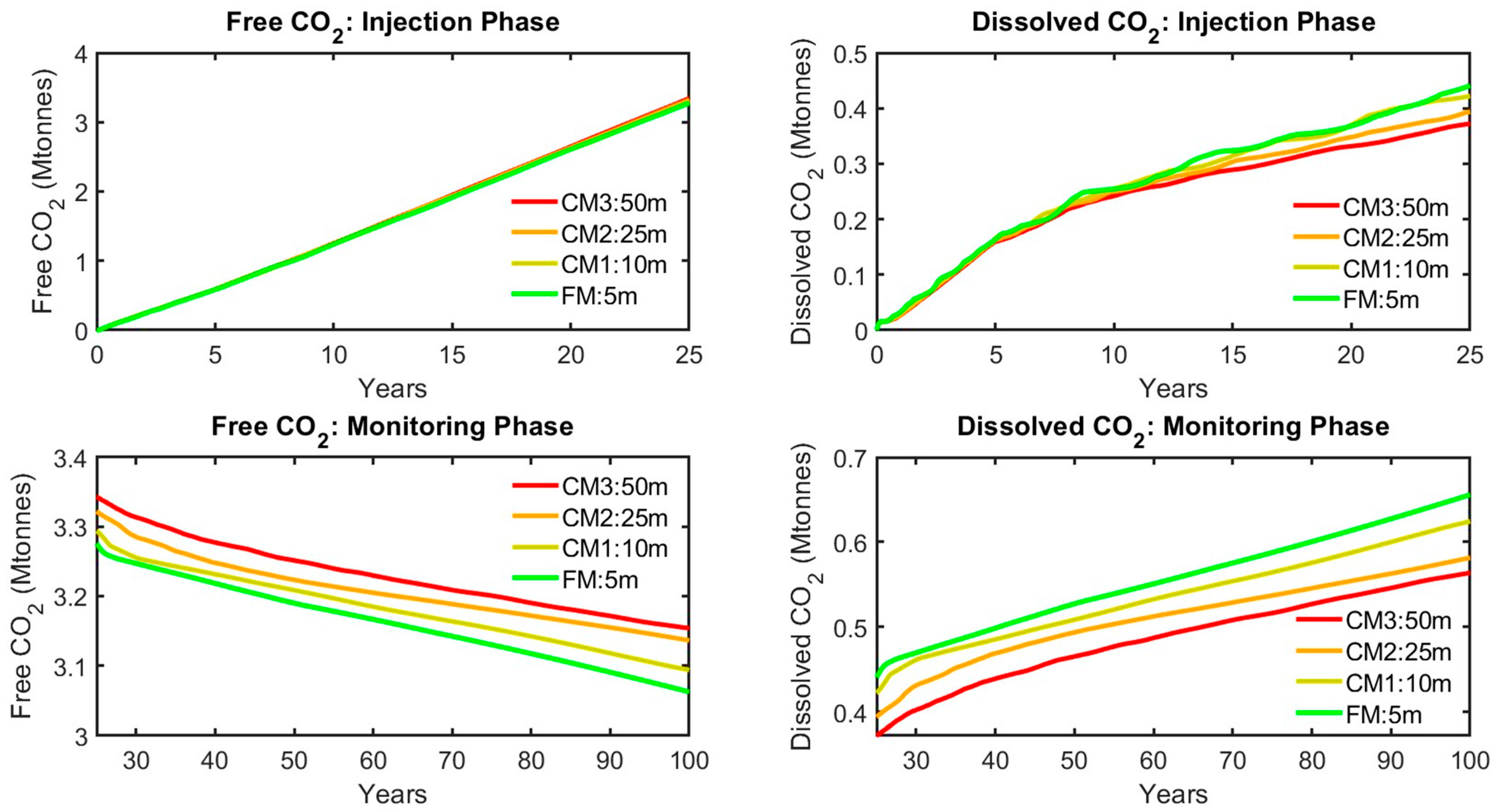
• CO₂ formation volume factor (B_g): Describes the compression and expansion of the free CO₂ phase as pressure changes throughout the different stages of the CCS project (injection, closure, and post-closure monitoring).

These parameters can be expressed mathematically using physical terms as follows:

$$R_s={\displaystyle \frac{V_{dCO2}^{sc}}{V_b^{sc}}}$$

(1)

$$B_b={\displaystyle \frac{V_b^{rc}}{V_b^{sc}}}={\displaystyle \frac{V_{dCO2}^{rc}+V_b^{rc}}{V_b^{sc}}}$$

(2)

where $V_{dCO2}^{sc}$ and $V_{dCO2}^{rc}$ are the volumes of dissolved CO₂ in formation brine at standard and reservoir conditions (P & T), respectively, and $V_b^{sc}$ and $V_b^{rc}$ are the formation brine volume at these conditions.

Rewriting these equations in terms of phase composition/equilibrium properties obtained from a thermodynamic model, the CO₂ solubility and the brine formation volume factor are expressed as:

$$R_s={\displaystyle \frac{V_{dCO2}^{sc}}{V_b^{sc}}}={\displaystyle \frac{{\overline{\rho }}_b^{sc}{x}_{CO2}}{{\overline{\rho }}_{CO2}^{sc}(1-x_{CO2})}}$$

(3)

$$B_b={\displaystyle \frac{V_b^{rc}}{V_b^{sc}}}={\displaystyle \frac{{\rho }_b^{sc}}{{\rho }_b^{rc}(1-{\omega }_{CO2})}}$$

(4)

where ${\overline{\rho }}_b^{sc}$ and ${\overline{\rho }}_{CO2}^{sc}$ are the molar densities of brine formation and CO₂ at standard conditions; $x_{CO2}$ is the CO₂ mole fraction in the aqueous phase; ${\rho }_b^{sc}$ and ${\rho }_b^{rc}$ are the mass densities of formation brine at standard and reservoir conditions, respectively; and ${\omega }_{CO2}$ is the CO₂ mass fraction in the aqueous phase.

Several models have been proposed to compute the aqueous solubility of CO₂, with or without considering water solubility in the CO₂ phase. Kumar (2004) [34] introduced an approach that combines correlations for binary interaction coefficients, volume shifts, and viscosity parameters as functions of temperature and salinity. This model is particularly effective for CO₂–brine systems, as it accounts for the influence of dissolved salts and high-pressure conditions. By proposing these correlations, Kumar’s work highlights the importance of calibrating Equation of State (EoS) parameters to ensure reliable predictions. These correlations enable the adjustment of interaction coefficients for nonidealities introduced by salinity and provide a framework for capturing pressure- and temperature-dependent effects on phase behavior.

Meanwhile, in this work, we employ the methodology outlined by Ismail et al. (2024) [13], which integrates various models to generate PVT data for carbon storage in saline aquifers. Specifically, this includes the work of Spycher et al. (2003, 2005, 2010) [32,35,36], which extends solubility calculations to account for the effects of temperature (up to 300 °C) and brine salinity. The approach by Spycher et al. 2003 [35] reformulates the equality of chemical potentials using “true” equilibrium constants for reactions between phases, incorporating corrections for nonideality in the liquid phase due to dissolved salts. Key parameters, such as the equilibrium constants, are defined as functions of temperature and pressure, with pressure corrections applied for deviations from the standard state. To compute CO₂ solubility in the aqueous phase and H₂O solubility in the CO₂-rich phase in the presence of salts, Spycher and Pruess (2005) [32] expanded their model by including activity coefficients for aqueous CO₂ and corrections to water activity to reflect the influence of salts. This required computation of the fugacity coefficient using an Equation of State (EoS), such as the modified Redlich–Kwong (RK) EoS, which was specifically tuned for H₂O–CO₂ systems. The activity coefficient for aqueous CO₂ was derived using the Duan and Sun (2003) [33] model, which incorporates both temperature and pressure dependencies for a broad range of conditions (temperature up to 260 °C, pressure up to 2000 bars, and varying salinity). Spycher et al. (2010) [36] further refined the model to cover temperatures up to 300 °C by adding expressions for activity coefficients and modifying equilibrium constant regressions for T > 100 °C. This tuning ensured accurate solubility predictions for high-temperature and high-pressure systems, particularly at elevated CO₂ concentrations where activity coefficients deviate from unity. Furthermore, the mixing rules for the RK EoS were adapted to include asymmetric binary interaction parameters for applications above 100 °C. While the Duan and Sun model performed well up to 260 °C, Spycher et al. adopted the Pitzer formalism [37] to address deviations at 300 °C, ensuring consistent accuracy across the extended temperature range. The adopted thermodynamic models—Spycher and Pruess (2005) [32] and Duan and Sun (2003) [33]—have been rigorously validated against experimental data as documented in their original publications, ensuring their reliability for the intended applications in this study.

Within the P–T range of interest (up to 600 bars, 300 °C), the combined approach enables robust and accurate predictions of CO₂ and H₂O phase behavior under conditions relevant to carbon storage in saline aquifers. By integrating these models, a comprehensive framework for analyzing PVT data, accommodating the complex interplay of temperature, pressure, and salinity, is obtained. By integrating Equations (3) and (4) with the thermodynamic model, the necessary PVT data for the BoM—including CO₂ solubility (R_s) and the brine formation volume factor (B_b) as a function of pressure—can be computed. Additional parameters, such as the CO₂ formation volume factor (B_g) and viscosity, are computed by MRST’s “CO2props” function, which covers pressures from 0.1 to 400 MPa and temperatures from 278 to 524 K. Brine properties, including density and viscosity, are derived from the correlations of Rowe and Chou (1970) [38] and Kestin et al. (1981) [39], accounting for salinity.

Finally, it is important to note that the BoM approach in this work focuses on carbon storage in saline aquifers, which offer vast storage capacities and have been utilized in notable projects such as Sleipner and Snøhvit in Norway, as well as the pioneering Northern Lights/Longship project. This method is particularly well-suited for two-phase systems typical in saline aquifer storage. However, for more complex scenarios, such as carbon storage in depleted oil fields where multiple phases (residual oil, hydrocarbon gas, brine, and CO₂) coexist, an extended Black Oil Model is necessary. This model would incorporate additional PVT data to accurately capture interactions between the various phases.

2.2. Comparative Analysis

Compositional modeling, which utilizes Equations of State (EoSs), offers a detailed and precise approach to simulating fluid behavior by accounting for interactions between multiple fluid components. EoSs describe the thermodynamic properties of these components, enabling the calculation of phase equilibria and fluid properties such as density and viscosity under varying conditions. This process involves solving complex nonlinear equations through iterative numerical methods. While this approach provides accurate phase behavior predictions, it must be tuned and demands significant computational resources and time. These computational requirements stem from the need to iteratively solve the equations while managing multiple fluid phases, thus requiring optimization to enhance efficiency, particularly for large-scale simulations.

Recognizing that many reservoir engineers rely on pre-tuned, off-the-shelf thermodynamic tools due to the lack of expertise or data for calibrating an EoS model, this study highlights the practicality of simplified models such as the Black Oil Model (BoM). While fluid models are a significant source of uncertainty, industry practice often prioritizes other uncertainties, such as reservoir size, shape, and relative permeability, particularly during capacity screening. Moreover, experimental PVT data is typically unavailable in the early stages of project development. This underscores the value of the BoM, which not only accelerates simulations but also accurately reproduces key parameters when paired with reliable EoS-derived or site-specific experimental data. In addition to its scientific focus, this work evaluates the strengths and weaknesses of fluid modeling options available in commercial simulation software. By shedding light on these modeling choices, the section aims to guide both practitioners and software developers in optimizing fluid simulation strategies.

In this section, we apply the previously described BoM methodology by generating PVT data for a case-specific aquifer and integrating it into the MRST black oil simulator. This framework simulates a carbon storage development scenario, and we assess the approach by comparing the results with those from three commercial simulators, all of which utilize compositional models with embedded EoSs. This contrasts with the BoM approach, which leverages EoSs offline to predict PVT data. The commercial simulators used for comparison and validation, along with their compositional models, are as follows:

• Eclipse E300 (Slb): Eclipse E300 is a widely used compositional simulator known for its versatility and accuracy in modeling complex fluid interactions. For carbon storage applications, Eclipse E300 employs advanced Equations of State such as the Peng–Robinson (PR) or Soave–Redlich–Kwong (SRK) EoS to model the thermodynamic behavior of CO₂ and reservoir fluids. It provides detailed phase behavior representation, making it highly effective for simulating CO₂ injection, migration, and trapping mechanisms. Eclipse E300 also includes features to model the dissolution of CO₂ in brine and its interactions with hydrocarbons, making it suitable for both saline aquifer and depleted reservoir scenarios.
• tNavigator (Rock Flow Dynamics): tNavigator is specifically designed for complex reservoir processes, including subsurface CO₂ storage. It employs sophisticated thermodynamic models and algorithms to simulate phase behavior and interactions of CO₂ with reservoir fluids. tNavigator is highly capable of handling multiple phases and components, allowing for precise simulations of CO₂ dissolution. Furthermore, tNavigator’s compositional model incorporates temperature and pressure effects on CO₂ solubility and phase behavior, making it a robust tool for CO₂ storage dynamics and risk mitigation.
• CMG-GEM (Computer Modeling Group): CMG-GEM is a leading compositional simulator designed for carbon storage and unconventional reservoirs. For carbon storage applications, CMG-GEM utilizes the Peng–Robinson Equation of State (EoS) to model the thermodynamics of CO₂ and reservoir fluids. One of CMG-GEM’s key features is its integration of geochemical modeling, which simulates mineral reactions and the potential for mineral trapping of CO₂. While Henry’s Law serves as the primary model for CO₂ dissolution in brine, CMG-GEM offers various options for modeling CO₂ solubility. The selection of a specific model is user-dependent and should correspond to the CO₂ stream composition, as well as the aquifer’s conditions and chemistry. This flexibility allows for tailored simulations that account for different geochemical and thermodynamic scenarios. These capabilities enable CMG-GEM to provide detailed simulations of CO₂–brine interactions and the long-term stability of stored CO₂. Additionally, its ability to model complex phase behavior, including CO₂–hydrocarbon interactions, makes CMG-GEM suitable for both saline aquifers and depleted oil and gas fields, ensuring effective and safe long-term CO₂ sequestration.

Under the conditions studied, all compositional simulators consistently predict a single CO₂-rich phase in equilibrium with the brine phase, confirming the validity of the comparison. Additionally, material balance errors were meticulously monitored throughout the simulations and maintained within acceptable thresholds to ensure the reliability and applicability of the results.

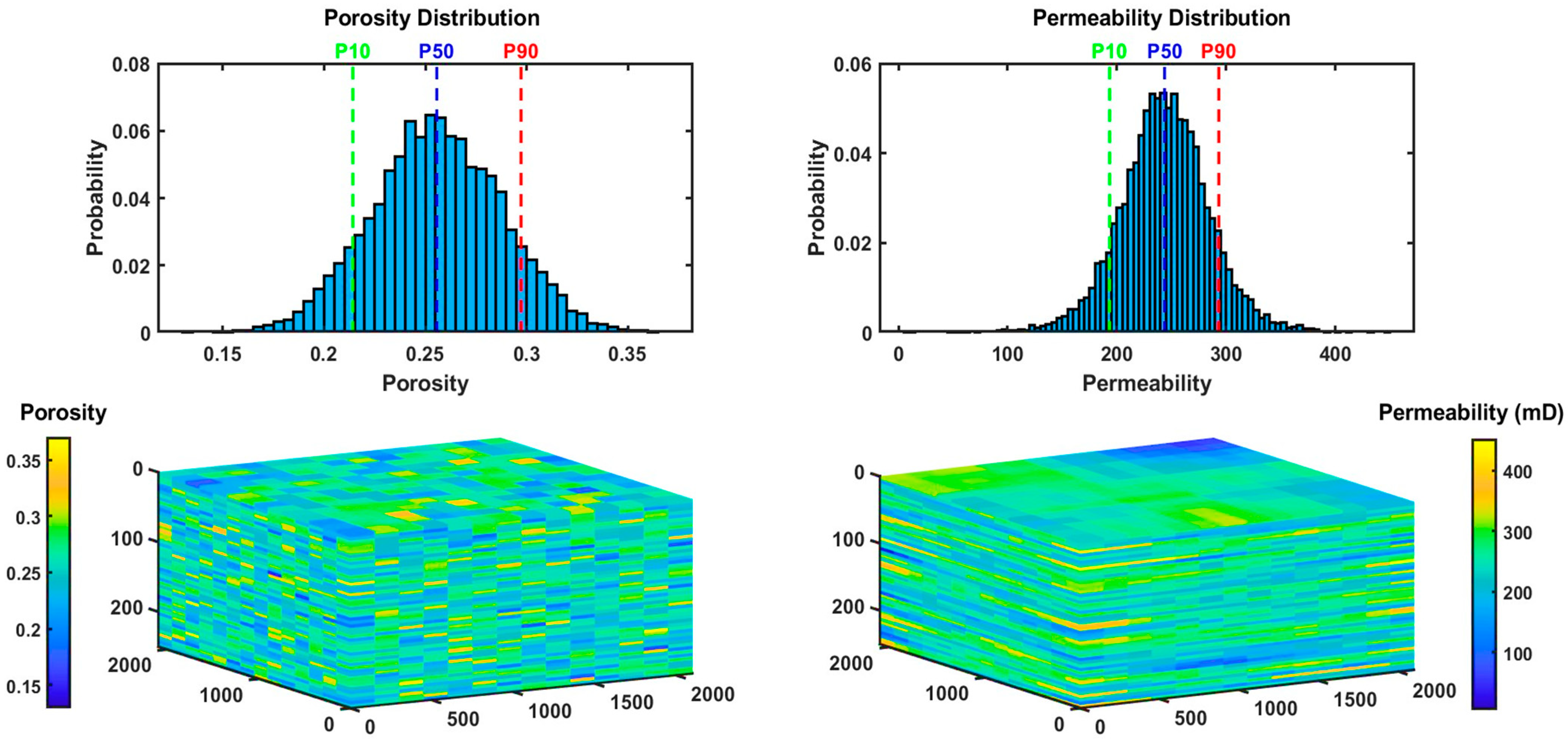
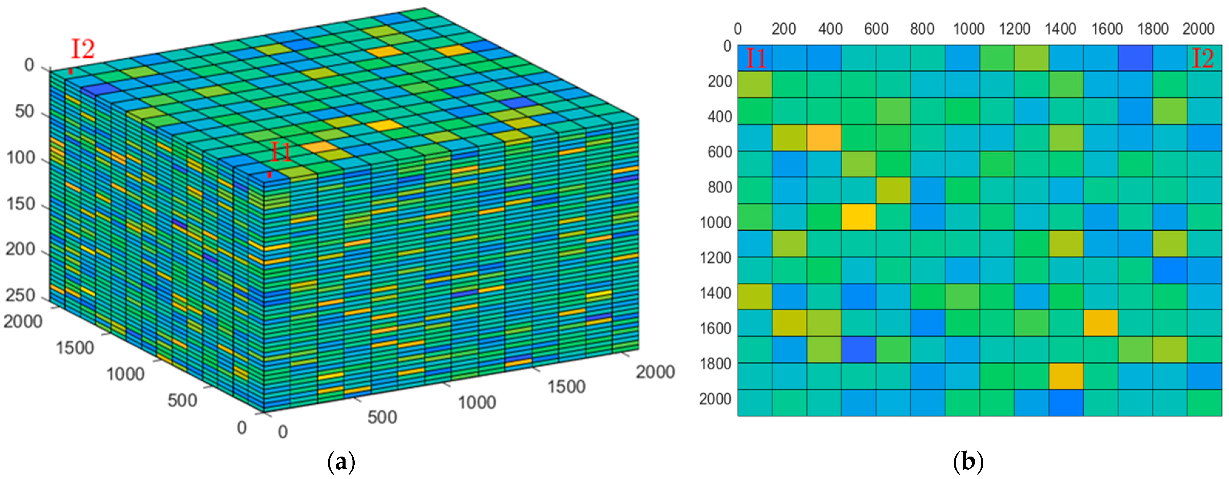
2.2.1. Simulation Setup

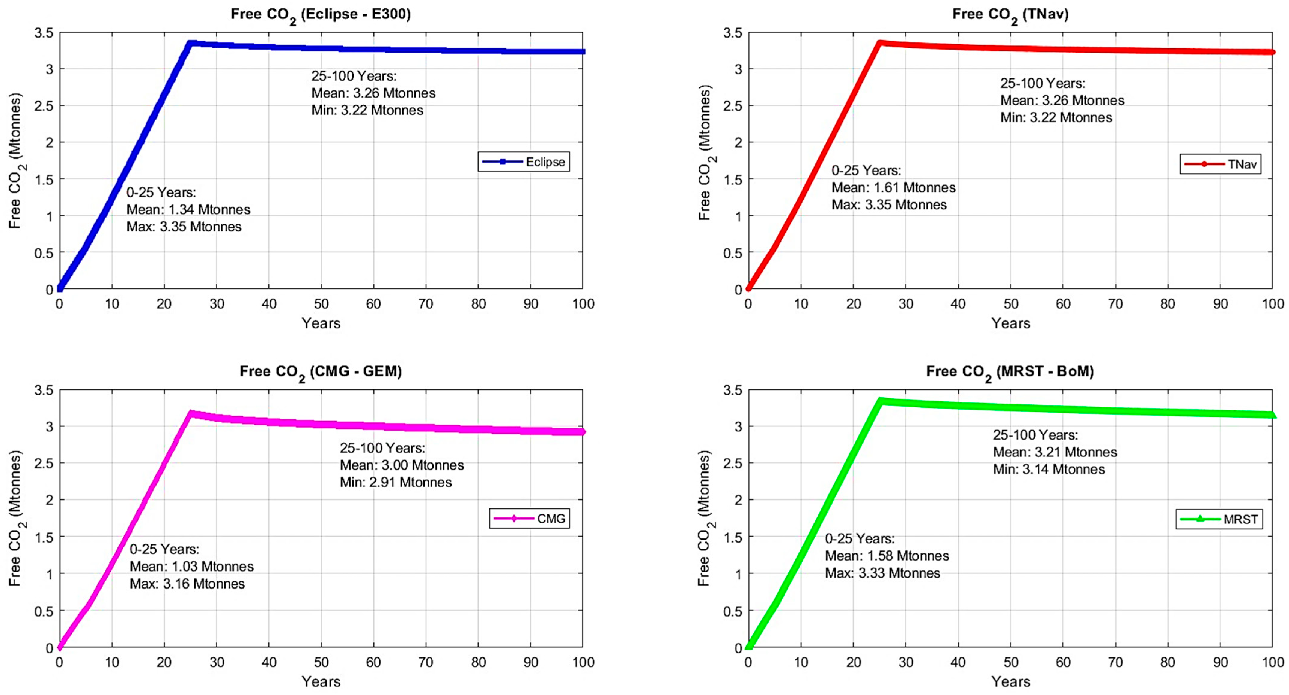
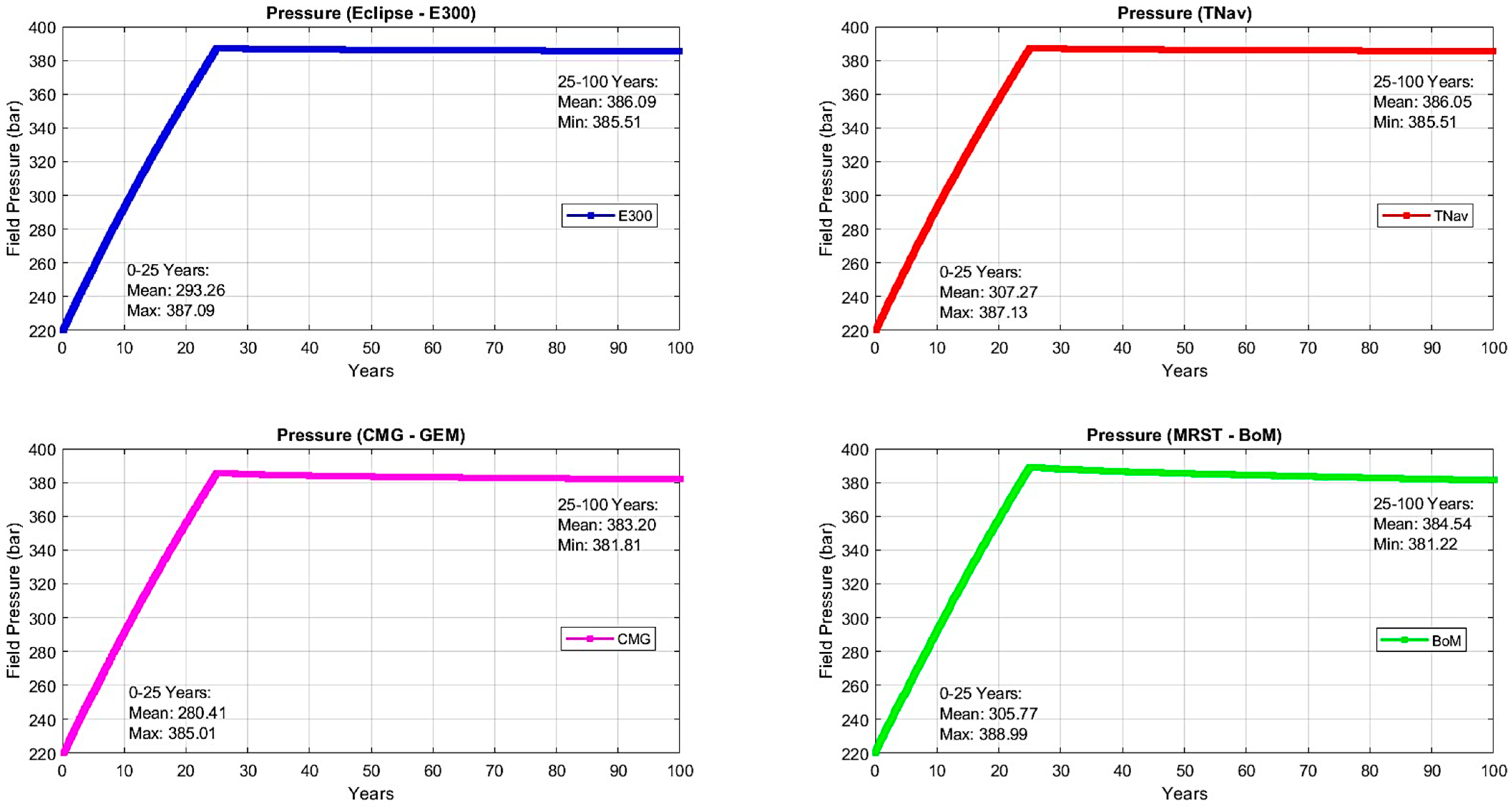
To evaluate the feasibility of applying the Black Oil Model (BoM) for simulating carbon storage in saline aquifer formations, we developed a simplified 3D Cartesian model. This model incorporates characteristics observed in significant commercial CCS projects worldwide, ensuring it represents a comprehensive spectrum of technical subsurface conditions. In building this model, we collected and analyzed data from various prominent CCS projects, assembling an inventory that includes key parameters such as porosity, permeability, thickness, and depth. The result is a model that reflects the full range of technical subsurface data, providing a robust foundation for evaluating the BoM’s performance in real-world scenarios. The simulated aquifer spans 2100 m in both length and width, with a maximum thickness of 250 m. The grid resolution is set to 150 m in the x- and y-directions, and 5 m in the z-direction, resulting in a grid configuration of 14 × 14 × 50 cells. The reservoir features Gaussian-distributed heterogeneity, with porosity values ranging from 13% to 37% and permeability ranging from 5 to 450 millidarcies. These ranges were selected to cover the diversity of subsurface conditions observed across multiple large-scale CCS projects, including values seen in the Sleipner and Snøhvit fields, which represent the forefront of CO₂ storage. The top of the reservoir is positioned at a depth of 1925 m, derived from the weighted average of various case studies, ensuring broad applicability across different geological settings. Figure 1 visualizes the reservoir properties and distribution.

The reservoir is assumed to be horizontally layered and isothermal, with a maximum temperature of 100 °C. Due to limited publicly available salinity data, we adopted a salinity value of 150,000 ppm, informed by data from the Lower Tuscaloosa Sandstone Formation in the SECARB Mississippi Pilot project. The top reservoir pressure is set at 206 bars. For relative permeabilities, we used a connate water saturation of 0.27 and a residual CO₂ saturation of 0.20. These values, applied uniformly across all simulators, were chosen based on industry best practices and validated data sources, further enhancing the relevance of the model for industry applications.

For the BoM case, the primary PVT data—such as the solution gas–oil ratio (modified to the CO₂–brine ratio) and the oil formation volume factor (adjusted to the brine formation volume factor)—were generated as functions of pressure, considering the specified reservoir characteristics (T = 100 °C, salinity = 150,000 ppm). Brine density at standard conditions and reservoir viscosity were determined using established correlations, while additional parameters, including standard density, reservoir viscosity, and the CO₂ formation volume factor, were computed using MRST’s CO2props built-in functions. Figure 2 presents the key PVT parameters generated and subsequently used for simulating carbon storage in this aquifer.

To prevent pressure drawdown from distorting the CO₂ plume’s shape and extent, we included only injection wells without any brine production wells. This setup ensures a closed aquifer system with no pressure relief, allowing for consistent control of the injection rate. A low injection rate was selected to maintain a stable plateau throughout the 25-year injection period (aligned with typical CCS permit durations), while ensuring that the bottom hole pressure did not exceed 500 bars at the injectors. This pressure limit corresponds to the maximum allowable pressure buildup, minimizing the need for simulators to adjust injection rates, which could otherwise impact the validation results. Two injection wells were strategically placed on one side of the reservoir (Inj 1: 1,1 and Inj 2: 1,14), with both configured to be rate-controlled. Figure 3 shows the well location in both 3D and 2D fashion. The wells injected 0.1 and 0.05 million metric tons per annum (Mtpa), respectively, into the last three layers (48–50), representing a 15 m-long perforation. The simulation spanned a 25-year injection period, followed by a 75-year post-closure monitoring phase, resulting in a total simulation time of 100 years.

To ensure consistency in comparing the BoM with compositional EoS modeling techniques, monthly time steps were used throughout all simulations. Although larger time steps could have sufficed during the post-closure equilibrium phase (due to slower changes in pressure and saturation), uniform time steps facilitated comparability between the operational and monitoring phases. The simplified model strikes a balance between capturing essential subsurface properties and avoiding unnecessary complexity. Excessive heterogeneity or intricate boundary conditions could obscure results, making multi-dimensional plume analysis challenging. This approach reflects typical challenges encountered in commercial CCS projects, laying a solid foundation for comparing the BoM with compositional models such as Eclipse E300, tNavigator, and CMG-GEM but also provide a consistent framework for evaluating the impact of grid resolution, as the same model is used for both aspects of this work.

2.2.2. Results

To assess the validity of the Black Oil Model (BoM) for simulating underground carbon storage in saline aquifers, we evaluated the results based on key aspects of carbon storage operations widely adopted in the industry. These aspects include the containment and security of in situ injected CO₂, with a focus on preventing leakage through pathways such as abandoned wells, faults, or open conduit fractures. A crucial component of this assessment is the risk evaluation based on the CO₂ plume’s evolution during the injection phase, post-closure, and the transfer of responsibility from the storage operator to the competent authority. Monitoring plans, corrective measures, financial security, and mechanisms are integral to this process. Therefore, our analysis primarily aimed to track the CO₂ plume’s evolution in terms of its extent and conformation over a 25-year injection period, followed by a 75-year post-closure monitoring phase. In addition to CO₂ plume behavior, we examined other key aspects of storage operations, such as pressure profiles and the characteristics of CO₂ dissolution and free gas-trapping mechanisms. These parameters are essential for understanding CO₂ behavior within the reservoir, which directly impacts storage capacity and integrity, as well as interactions with brine and the effectiveness of trapping mechanisms. Figure 4 compares the performance of the BoM with three commercial simulators—Eclipse E300, CMG-GEM, and TNav—by visualizing CO₂ saturation in the top reservoir layer across various time steps during both the injection and the monitoring phases. Although it would be more useful to select one of the models/simulators as a reference and present the plots of the differences in gas saturation for the others, allowing easier understanding to the reader, we believe that doing so could unintentionally imply a preference for or endorsement of that model. Since the compositional simulators used in this study (e.g., Eclipse, T-Navigator, and CMG-GEM) are well-established commercial tools widely used in industry, assigning one as a reference could inadvertently suggest that it is the most accurate, potentially introducing bias and indirect commercialism. Our aim is to provide a balanced comparison, allowing readers to assess the relative performance of each model without implying that one is superior to the others. This approach ensures the neutrality and objectivity of the study, leaving it to the reader or operator to determine which model aligns best with their specific requirements or field data.

Furthermore, we conducted a quantitative assessment of the consistency between the Black Oil Model and the compositional simulators by calculating the mean absolute error (MAE) in CO₂ saturation across the top reservoir layer. This error was computed at five critical time steps (10, 25, 50, 75, and 100 years), covering both the injection and the post-closure phases. The MAE was expressed as a percentage of the maximum saturation (0.73 considering the connate water saturation) to normalize across models. Rather than designating a single simulator as a ground truth, we adopted a benchmarking strategy whereby each compositional simulator’s results were compared against the corresponding BoM case. This ensured a fair and neutral basis for evaluating the BoM’s fidelity in capturing CO₂ plume dynamics. To offer a more integrative perspective, we also calculated average errors over the injection period (10 and 25 years) as well as the entire CCS project phase, injection, and monitoring timeline. This comparative analysis, summarized in

Table 1. Mean absolute error (%) in CO₂ saturation between the BoM and compositional simulators at key time steps in the injection phase and throughout the entire CCS timeline.

	Injection Phase		Monitoring Phase			Average (Injection Phase and CCS Timeline)
Model	10 Years	25 Years	50 Years	75 Years	100 Years	T1–T25	T1–T100
E300	2.01%	4.13%	4.18%	4.94%	5.50%	3.07%	4.15%
CMG	0.52%	2.38%	4.56%	4.57%	4.81%	1.45%	3.37%
TNav	3.08%	3.41%	3.60%	4.38%	4.94%	3.24%	3.88%

, reveals consistent trends and highlights both the robustness and the limitations of the BoM across different temporal scales and simulator types.

Considering Figure 4, during the initial 10 years of CO₂ injection, the BoM reports a mean saturation value of 0.05, aligning closely with the mean saturation of 0.05, 0.06, and 0.07 for CMG-GEM, E300, and TNav, respectively. Across all models, the CO₂ plume is concentrated in the upper-left region of the reservoir, indicating the BoM’s effectiveness in capturing early-stage CO₂ migration and plume development. The minor variations in saturation values can be attributed to differences in model parameters and assumptions, though they remain within acceptable limits. At the 25-year mark, the BoM’s mean saturation rises to 0.21, comparable to TNav (0.23) and CMG-GEM (0.19), while Eclipse E300 records a higher value of 0.24. This phase illustrates the BoM’s capability to effectively simulate CO₂ injection dynamics, particularly with regard to lateral plume spread and dissolution into brine. Overall, the close alignment of results during the injection period supports the reliability of the BoM technique for modeling CO₂ storage over the project’s injection phase.

As the simulation progresses into the mid- to late monitoring period (50 years)—a phase typically associated with the transfer of responsibility from operators to regulatory authorities, where the reliability of the dynamic model is crucial—the BoM continues to produce results consistent with the commercial compositional simulators. The mean CO₂ saturation in the BoM reaches 0.35, compared to 0.38 for both Eclipse E300 and TNav, and 0.32 for CMG-GEM. Qualitatively, the plume distribution remains similar across the BoM, Eclipse E300, and TNav, while CMG-GEM exhibits slightly lower saturation due to its CO₂ dissolution model based on Henry’s Law. At the 75-year checkpoint, the BoM’s mean saturation stabilizes at 0.40, closely matching those of TNav (0.44) and Eclipse E300 (0.44), while CMG-GEM reports a slightly lower value of 0.37. By the end of the simulation (100 years), the BoM reaches a final saturation of 0.44, slightly lower than those of TNav (0.47) and Eclipse E300 (0.48), but higher than that of CMG-GEM (0.40). The qualitative plume extent remains comparable across all models, reinforcing the BoM’s effectiveness in modeling long-term CO₂ sequestration dynamics.

In addition to comparing the BoM with commercial simulators, it is valuable to assess the differences among the simulators themselves—Eclipse E300, CMG-GEM, and TNav—to provide insights for operators adopting these tools for site characterization and scenario development. While these simulators exhibit broadly similar CO₂ behavior and plume dynamics, slight variations in saturation levels and plume extent emerge due to differences in their tuned Equations of State (EoSs) and solubility models. E300 tends to predict slightly higher saturation values and more extensive CO₂ plumes compared to the other simulators. This can be attributed to its advanced use of tuned EoSs, such as the Peng–Robinson and Soave–Redlich–Kwong models, which offer a detailed representation of phase behavior, leading to higher predicted levels of CO₂ retention in the reservoir. TNav follows closely behind Eclipse E300 in terms of predicted saturation values and plume extent. CMG-GEM reports slightly lower CO₂ saturation levels compared to both Eclipse E300 and TNav. This difference does not reflect a higher or lower accuracy of CMG-GEM but rather stems from the solubility model it employs. Specifically, CMG-GEM uses Henry’s Law for modeling CO₂ dissolution, which predicts higher CO₂ solubility in brine. This leads to greater dissolution and, consequently, smaller CO₂ plumes over time. Despite these slight variations in predicted saturation levels and plume behavior, all the simulators demonstrate a high degree of consistency in their overall performance.

To quantitatively evaluate CO₂ storage performance using the BoM model, we first assessed the mean absolute error (MAE) in CO₂ saturation between the BoM and compositional simulators, focusing on the first layer. Since Table 1 presents the same data as Figure 4 but in a numerical format, we refrained from a separate detailed discussion here. Additionally, the evolution of both free-phase and dissolved CO₂ was examined and is presented in Figure 5 and Figure 6.

Figure 5 and Figure 6 summarize these profiles, providing insights into the capability of the BoM technique describing the behavior of CO₂ during the injection and post-closure monitoring phases.

As shown in Figure 5, during the initial injection phase (0–25 years), all four models display the expected rapid increase in free CO₂. Eclipse E300 and TNav both reach peaks of 3.35 Mt, with mean values over time tracking the shape of the increase in the order of 1.34 Mt and 1.61 Mt, respectively. The MRST BoM demonstrates strong consistency with these models, reaching 3.33 Mt, with a mean value of 1.58 Mt, showing that the BoM closely follows the behavior of well-established simulators in the early injection phase. In contrast, CMG-GEM exhibits a slightly lower peak of 3.16 Mt, with a mean value of 1.03 Mt, due to its use of the different solubility model of Henry’s Law, which in turn affects the availability of free CO₂ in the system. In the post-closure monitoring phase (25–100 years), free CO₂ levels begin to stabilize and gradually decrease as the CO₂ plume propagated further into the reservoir and encountered fresh brine, leading to further dissolution. By the end of the simulation (100 years), Eclipse E300 and TNav both stabilize around 3.22 Mt, with a mean value of 3.26 Mt, while the MRST BoM settles at 3.14 Mt, with a mean of 3.21 Mt. CMG-GEM stabilizes at a slightly lower level of 2.91 Mt, with a mean of 3.00 Mt.

These stabilization trends confirm that the BoM performs consistently with alternative compositional models during the long-term containment phase. The BoM’s ability to track free CO₂ dynamics with only minor differences from compositional models validates its effectiveness in capturing CO₂ behavior over time, supporting its use as a computationally efficient alternative.

The dissolved CO₂ profiles in Figure 6 provide further validation of the BoM’s ability to simulate CO₂ sequestration. During the initial injection phase (0–25 years), Eclipse E300 shows a steady increase in dissolved CO₂, reaching 0.40 Mt, with a mean value of 0.23 Mt. TNav follows a similar trend, also reaching 0.40 Mt, with a mean value of 0.27 Mt. The MRST BoM demonstrates similar behavior, peaking at 0.39 Mt, with a mean value of 0.24 Mt, closely aligning with both Eclipse E300 and TNav. In contrast, CMG-GEM shows a rapid initial increase, leveling off at a higher maximum of 0.88 Mt, with a mean value of 0.31 Mt, reflecting its enhanced solubility model. In the post-closure monitoring phase (25–100 years), Eclipse E300 and TNav continue to show gradual increases in dissolved CO₂, both reaching about 0.49 Mt, with similar mean values. The MRST BoM follows a comparable trend, reaching 0.50 Mt, with a mean of 0.50 Mt. CMG-GEM, however, stabilizes at a higher level of 0.79 Mt, indicating stronger dissolution of CO₂ into the brine. These results demonstrate that the BoM is effective in modeling long-term CO₂ dissolution dynamics, consistent with both Eclipse E300 and TNav, further validating the BoM as a reliable tool for simulating CO₂ behavior.

The combined analysis of free and dissolved CO₂ profiles reveals that while all models effectively simulate CO₂ injection and stabilization, the MRST BoM consistently provides similar results to those of Eclipse E300 and TNav, particularly in terms of plume behavior and storage dynamics. Although minor quantitative differences exist with CMG-GEM, attributed to its different solubility model, the BoM remains well within the expected range of behavior for CO₂ sequestration. This analysis underscores the importance of understanding the specific assumptions and solubility models used by each simulator. By validating the BoM against the compositional models in Eclipse E300, TNav, and CMG-GEM, we demonstrate that the BoM provides an accurate and computationally efficient alternative for simulating CO₂ storage. Its ability to capture the essential dynamics of both free and dissolved CO₂ reinforces its value for long-term simulations, offering operators and regulators a reliable tool for risk evaluation and strategic planning.

To enhance the validation of the BoM as a reliable model, the field pressure profiles during the injection and post-injection phases (as shown in Figure 7) provide critical insights into CO₂ storage performance across the different simulators. During the injection phase, all models exhibit the expected rapid increase in field pressure, demonstrating consistent behavior in response to CO₂ injection. Eclipse E300 records a mean pressure over time in the order of 293.26 bar, peaking at 387.09 bar, while TNav follows closely with a mean of 307.27 bar and a maximum of 387.13 bar. The MRST BoM demonstrates similar behavior, with a mean pressure of 305.77 bar and a peak of 388.99 bar, aligning well with both Eclipse E300 and TNav. CMG-GEM exhibits a slightly lower mean pressure of 280.41 bar and a peak of 385.01 bar due to the pressure-relieving effect of CO₂ dissolution in the brine. These results indicate that the BoM can effectively simulate pressure buildup during CO₂ injection, closely matching the performance of more computationally intensive compositional models.

In the post-closure monitoring phase, field pressure levels for Eclipse E300, TNav, and MRST stabilize, exhibiting minimal fluctuations, primarily due to the continued dissolution of CO₂ into fresh brine. This dissolution reduces the compressible phase in the reservoir, leading to a gradual decrease in pressure levels. Eclipse E300 stabilizes with a mean pressure of 386.09 bar, TNav records 386.05 bar, and the MRST BoM settles at 384.54 bar. CMG-GEM, however, stabilizes at a slightly lower mean pressure of 383.20 bar, reflecting the lower amount of free CO₂ in the system, as discussed earlier. These stable pressure levels during the post-injection phase indicate a balanced reservoir state, which is crucial for the long-term containment of CO₂. The slight variations in pressure stabilization among the models reflect their unique approaches to modeling CO₂ behavior and interactions within the reservoir, particularly in how they account for factors like CO₂ dissolution and phase interactions.

Overall, when considered alongside the earlier results—such as plume extension, conformance predictions, and storage mechanisms—the analysis affirms that the BoM approach is a reliable and effective method for simulating carbon storage in saline aquifers. The consistency of the BoM technique results, both qualitatively and quantitatively, demonstrates its robustness and further validates its application in modeling CO₂ storage further enhancing the deployment of CCS projects.

3. Grid Resolution Impact Assessment

During the injection phase, CO₂ displaces brine, and after injection ceases, it continues to migrate upwards due to buoyancy forces. This bulk-phase movement, combined with various trapping mechanisms, plays a crucial role in determining the extent and dynamics of the CO₂ plume, ultimately impacting all operational aspects of carbon storage. Accurate simulations, often requiring fine-scale modeling, are essential, as they directly influence the effectiveness of monitoring and management strategies designed to ensure safe and efficient CO₂ storage. Fine-scale modeling captures critical geological features such as caprock integrity, plume migration, and dissolution dynamics, providing the level of detail necessary for risk assessment and operational decision-making.

To address the computational challenges posed by fine-scale modeling, operators and storage developers frequently apply upscaling techniques to implement coarser grid resolutions. Upscaling reduces the computational burden by averaging petrophysical properties such as porosity and permeability over larger grid blocks, simplifying the model while maintaining the overall trends in geological features. One benefit of upscaling is the elimination of small-scale features, such as pinch-out cells—zones where the reservoir thickness tapers to zero—which can complicate fluid flow simulations and introduce instability in numerical models. While the removal of such features can streamline computations, it also risks oversimplifying areas of complex geometry, potentially leading to inaccuracies in simulating CO₂ plume migration and trapping mechanisms. The balance between computational efficiency and simulation accuracy is therefore critical. Consequently, understanding how grid resolution affects critical aspects of CO₂ behavior—such as plume extent, trapping mechanisms, and storage site integrity—is essential to ensuring the accuracy and reliability of in situ CO₂ models. Gaining this understanding enhances model fidelity and supports effective project development, monitoring, and, ultimately, compliance with environmental safety and regulatory requirements.

Having verified the validity of the Black Oil Model (BoM) in the previous section, this part of the study focuses on investigating the impact of grid resolution. We compare several upscaled models, adjusted in both the vertical (z) and lateral (x and y) dimensions, against a fine-scale reference model. Through these comparisons, we propose a flexible evaluation criterion applicable to various CCS projects, allowing for the assessment of the effectiveness of upscaled models in real-world scenarios. This section is organized into three parts. First, we discuss the upscaling techniques and coarse models developed for the comparison. Next, we focus on upscaling along the vertical direction (z) and evaluate the performance of upscaled models relative to the fine-scale reference. Finally, we examine the effects of upscaling in the lateral directions (x and y) and compare the performance of the upscaled models with the fine-scale model. The aim of this section is to demonstrate the impact of grid resolution on CO₂ storage simulations, so that project operators and regulators can better assess the trade-offs between computational efficiency and model accuracy. This section aims to inform on the trade-off between computational cost and model accuracy for large-scale CCS simulations. In particular:

1-

Quantifying Impact: This section highlights the acceptable thresholds for coarsening grids while maintaining accuracy, which is critical for large-scale simulations where computational resources are constrained.

2-

Understanding Limitations: It demonstrates that while coarse grids are suitable for some applications, certain scenarios (e.g., monitoring fine-scale plume migration) require higher resolution, emphasizing the need for targeted refinement.

3-

Guidance for Operators: By providing a clear understanding of grid resolution impacts, this section offers practical guidance to operators on optimizing grid design for different simulation objectives.

3.1. Coarse Model Development & Evaluation Criteria

The upscaling of petrophysical properties, specifically porosity and permeability, is essential for adjusting datasets across different modeling scales while preserving the critical geological characteristics of the subsurface. The proposed meshing strategy is based on the Finite Volume Method (FVM), which is widely used in reservoir simulation for its robustness. In this framework, the governing partial differential equations ensure mass, momentum, and energy conservation. By applying both spatial and temporal discretization, the differential equations are turned into a system of non-linear algebraic ones so that at the control volume level (i.e., each cell) pressure varies according to the mass change, which in turn is controlled by the treatment of fluxes across cell interfaces, as dictated by Darcy’s Law. Note that thermal calculations through the application of an energy balance do not apply since the reservoir is isothermal. The resulting algebraic equations at each discretized time step are solved iteratively using a classic Newton–Raphson approach allowing for a balance between numerical accuracy and computational efficiency. This approach was followed to assess the coarse mesh effect and compared against a fine-scale one to evaluate how the physical processes are captured. Uniform upscaling was implemented on purpose to provide a straightforward and consistent approach to isolate and evaluate the influence of grid resolution on critical parameters such as plume migration, dissolution, and pressure distribution. Adopting more complex upscaling methods could introduce additional variables unique to the chosen methodology, potentially complicating the interpretation of results and obscuring the direct relationship between grid resolution and simulation outcomes. Furthermore, for large-scale CCS simulations in saline aquifers—where available geological data is often sparse, and formations are typically approximated as moderately heterogeneous— uniform upscaling remains a practical and widely adopted approach. It facilitates clear and unbiased comparisons across different grid resolutions and simulation models while accommodating the inherent limitations in data availability. Based on that, permeability values (k_x, k_y, k_z) and porosity were extracted as 1D arrays and reshaped into 3D matrices to align with the spatial dimensions of the original rock sample. The finest-scale model, as previously discussed, was represented by a 14 × 14 × 50 cell grid, capturing the detailed heterogeneity of the subsurface environment.

To reduce computational complexity, the 3D matrices were systematically downsampled by averaging values over blocks in both the vertical (z) and lateral (x and y) directions. This approach enabled a reduction in grid resolution while retaining key geological trends and patterns, ensuring that critical subsurface properties influencing CO₂ migration and trapping mechanisms were preserved. For each upscaling direction, progressively coarser models were generated to evaluate how grid resolution impacts the accuracy of simulation results, particularly with regard to CO₂ plume behavior.

For z-direction upscaling, the x and y grid dimensions were held constant at 150 m, while the z-direction grid size was varied. Conversely, for x- and y-direction upscaling, the z-direction grid size was fixed at 5 m to assess the impact of lateral resolution on simulation outcomes. The fine-scale model used in this analysis is the same model discussed in the previous section, with the following details and summarized in

Table 2. Grid model summary.

Model Name	Grid Dimensions	Number of Cells	Z-Direction Grid Size	X-/Y-Direction Grid Size
Fine Model (FM)	14 × 14 × 50	9800	5 m	150 m
Coarse Model (CM1)	14 × 14 × 25	4900	10 m	150 m
Coarse Model 2 (CM2)	14 × 14 × 10	1960	25 m	150 m
Coarse Model 3 (CM3)	14 × 14 × 7	980	50 m	150 m
Coarse Model 4 (CM4)	12 × 12 × 50	7200	5 m	175 m
Coarse Model 5 (CM5)	10 × 10 × 50	5000	5 m	210 m
Coarse Model 6 (CM6)	7 × 7 × 50	2450	5 m	300 m

:

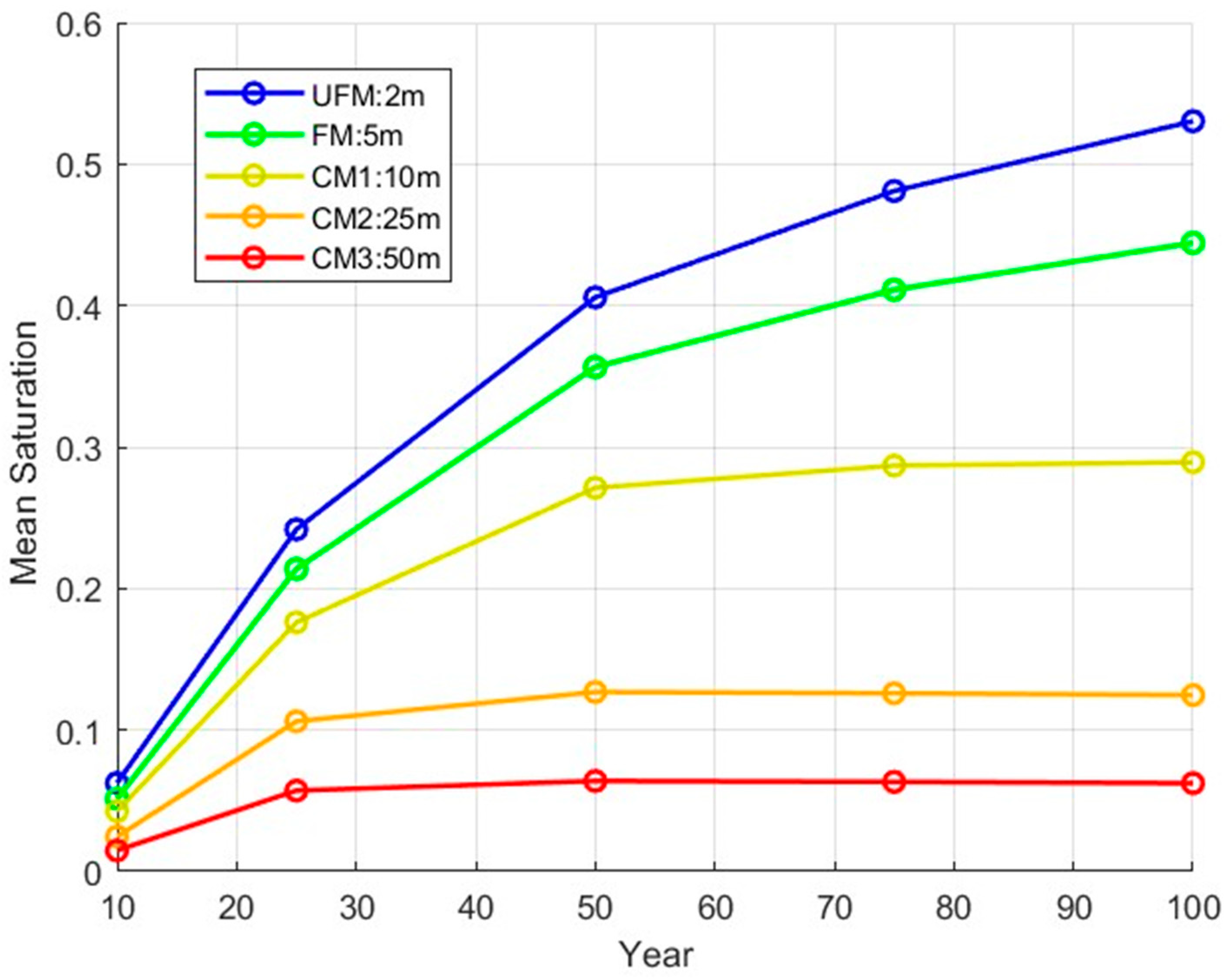
• Fine Model (FM): 14 × 14 × 50 grid—9800 cells—z-direction grid size: 5 m; x, y grid size: 150 m.

The following summarizes the upscaled models generated in the z-direction:

• Coarse Model 1 (CM1): 14 × 14 × 25 grid—4900 cells—z-direction grid size: 10 m; x, y grid size: 150 m.
• Coarse Model 2 (CM2): 14 × 14 × 10 grid—1960 cells—z-direction grid size: 25 m; x, y grid size: 150 m.
• Coarse Model 3 (CM3): 14 × 14 × 7 grid—980 cells—z-direction grid size: 50 m; x, y grid size: 150 m.

For x- and y-direction upscaling, the following models were developed with the z-direction grid size fixed:

• Coarse Model 4 (CM4): 12 × 12 × 50 grid—7200 cells—x, y grid size: 175 m; z-direction grid size: 5 m.
• Coarse Model 5 (CM5): 10 × 10 × 50 grid—5000 cells—x, y grid size: 210 m; z-direction grid size: 5 m.
• Coarse Model 6 (CM6): 7 × 7 × 50 grid—2450 cells—x, y grid size: 300 m; z-direction grid size: 5 m.

To assess the performance of these upscaled models, a hybrid evaluation approach was employed, incorporating both qualitative and quantitative assessments, similar to the methodology used in validating the Black Oil Model as a viable technique for simulating carbon storage in saline aquifers.

The qualitative evaluation focused on the predicted extent and shape of the CO₂ plume. For storage operators, the extent of the plume is critical in guiding injection strategy and assessing project viability. It also impacts risk assessment and monitoring protocols, particularly in determining the scope of the Monitoring, Measurement, and Verification (MMV) plan. This includes decisions on which areas require more intensive monitoring, the duration of monitoring, and the technologies to be employed. For regulators, ensuring that the CO₂ plume remains within the designated storage site is crucial for preventing leakage, which could harm surrounding environments or communities. Furthermore, the plume’s predicted extent influences financial security measures, as operators must allocate funds to cover potential corrective actions if containment fails. The larger the plume or the higher the risk, the greater the financial security required.

The quantitative evaluation considered two critical aspects: the pressure profile of the reservoir and the trapping mechanisms during both the injection and post-closure phases. The pressure profile directly influences several operational and safety factors. For storage operators, accurately modeling the pressure distribution within the storage site is vital for determining the maximum injection rate, overall storage capacity, and injectivity of the reservoir. Misjudging the pressure dynamics can lead to excessive pressure buildup, which might compromise the integrity of the storage formation or the caprock, potentially causing geomechanical issues such as fault reactivation or wellbore integrity problems. From the regulatory perspective, the pressure profile is a critical safety parameter. Ensuring that the pressure remains within safe limits is necessary for maintaining long-term CO₂ containment and preventing breaches that could lead to leakage. Pressure dynamics also have important implications for regulatory oversight, especially regarding the long-term liability of storage sites. Operators are required to demonstrate that pressures will not induce unsafe conditions throughout the project’s lifecycle, ensuring both short-term operational safety and long-term site stability. In addition to pressure dynamics, the evaluation also considered trapping mechanisms involved in CO₂ storage. Understanding how CO₂ is sequestered in the reservoir provides valuable insights into the overall security of the storage process. Free-phase CO₂, which remains mobile, poses a higher risk of leakage and, therefore, requires more rigorous monitoring and intervention strategies. On the other hand, dissolved CO₂, securely trapped in the brine phase, offers much greater assurance of long-term containment and stability. The evolution of these trapping mechanisms is critical for both risk management and operational decision-making. Storage operators need to carefully monitor how the balance between mobile and immobile CO₂ changes over time, particularly during the transition from active injection to the post-closure phase. For regulators, the progression of trapping mechanisms offers insight into the long-term containment security of CO₂, influencing regulatory decisions around monitoring duration, liability periods, and potential remedial actions if containment is compromised.

This comprehensive framework allows for a thorough assessment of the balance between maintaining sufficient accuracy and achieving computational efficiency in CO₂ storage modeling.

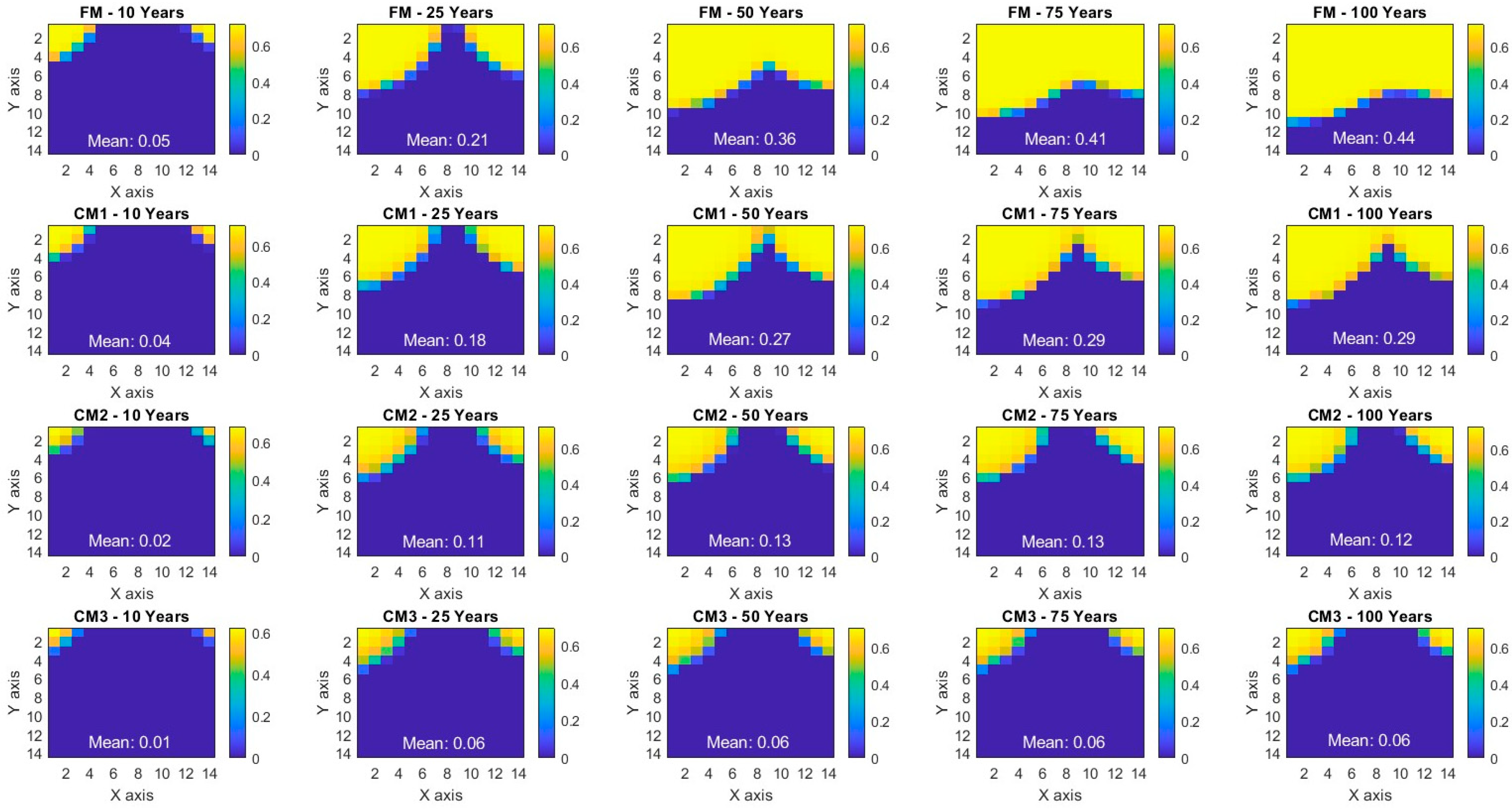
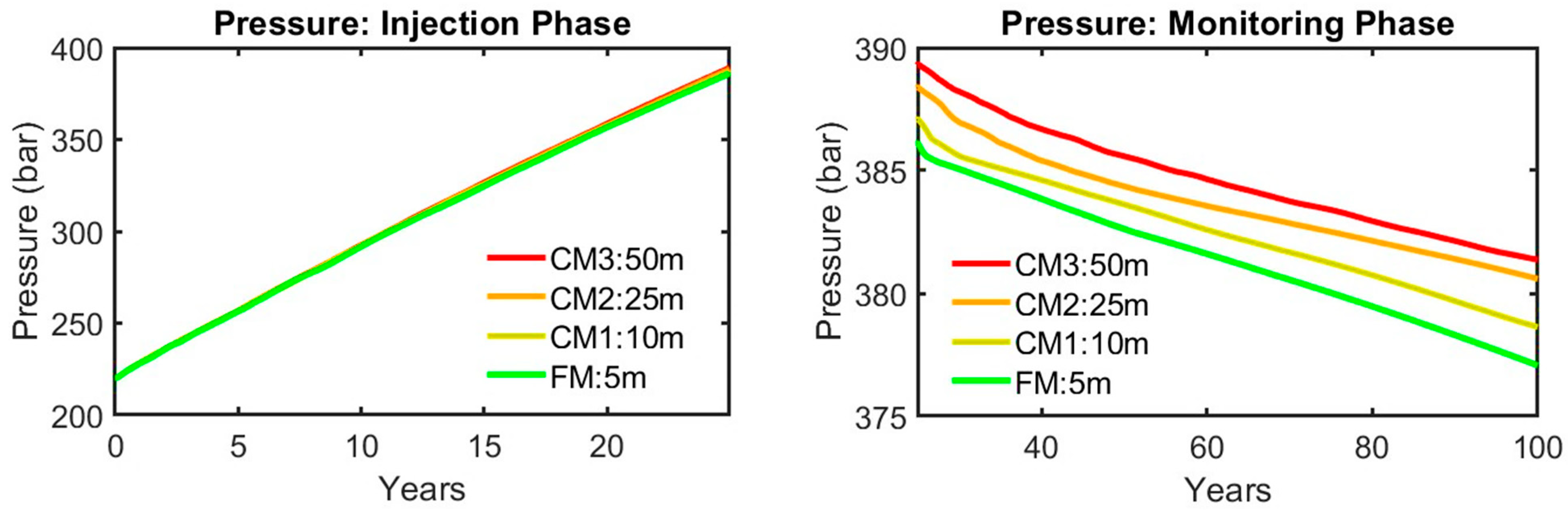
3.2. Vertical Upscaling—Grid Resolution Impact in the Z-Direction

To evaluate the impact of vertical upscaling, the same development and injection scenario previously discussed was adopted, with a slight modification to the injection strategy. Specifically, the perforation of the injection wells was restricted to the lower 50 m of the reservoir. This adjustment was made to accommodate a unique injection scenario along the variations in grid cell thickness across models, ensuring consistency and facilitating a fair comparison between different models.

Figure 8 illustrates the impact of various vertical grid resolutions on the predicted CO₂ plume extent in the top reservoir layer, assessed at multiple time steps during both the operational phase (10 and 25 years) and the post-injection monitoring phase (50, 75, and 100 years). Focusing on the top layer directly beneath the caprock allows for a simplified interpretation of the results, avoiding the complexities of 3D visualization. This layer is particularly critical due to the high buoyancy of the migrating CO₂, making it an ideal choice for assessing the effectiveness of different grid resolutions. During the first 10 years of injection, the Fine Model (FM) captures a small but distinct CO₂ plume, with a mean saturation over the top layer of 0.05. In contrast, Coarse Model 1 (CM1), with a 10 m vertical grid size, shows a slightly smaller plume with a mean saturation of 0.04. Coarse Model 2 (CM2) presents an even smaller plume, with a mean saturation of 0.02, indicating a loss of detail in capturing plume dynamics. Meanwhile, Coarse Model 3 (CM3) exhibits a negligible plume, with a mean saturation of 0.01, highlighting the limitations of excessive upscaling. By the 25-year mark, the FM demonstrates a significant increase in mean saturation to 0.21, illustrating substantial plume growth and pronounced upward migration of CO₂. CM1’s saturation rises to 0.18, reflecting some plume expansion falling slightly short of the FM’s effectiveness. CM2, with a mean saturation of 0.11, further underscores the limitations of coarser resolutions, while CM3’s saturation remains low at 0.06, indicating minimal plume growth and inadequate model performance. These findings underscore the risks of relying on highly coarse grids during the operational phase, as they may significantly underestimate the extent of the CO₂ plume, potentially affecting critical decisions related to injection operations and monitoring protocols.

In the early post-injection monitoring phase, 50 years after injection, the Fine Model (FM) displays a broader CO₂ plume, with a mean saturation of 0.36, indicating effective upward migration and plume development. CM1 shows a mean saturation of 0.27, reflecting continued plume expansion, though less extensive and more discontinuous compared to the FM. In contrast, CM2’s mean saturation is limited to 0.13, indicating inaccurate plume growth, while CM3 remains stagnant at 0.06, highlighting its inefficacy in capturing plume dynamics even at this stage. At 75 years, the FM reaches a mean saturation of 0.41, reflecting sustained plume growth. CM1’s saturation holds at 0.29, and although the plume continues to develop, it falls short of the FM’s accuracy in representing plume shape and extent. CM2 remains limited, with a mean saturation of 0.13, while CM3 continues at 0.06, underscoring its inability to model the evolving plume dynamics. By the 100-year mark, the FM demonstrates a mean saturation of 0.44, with CM1 showing 0.29, further indicating the limitations of coarser models in accurately representing long-term plume behavior. CM2 and CM3 remain at 0.12 and 0.06, respectively. The results clearly illustrate the significant impact of grid resolution on modeling accuracy during the post-injection monitoring phases, underscoring the necessity for careful consideration of grid resolution in CO₂ storage modeling.

Overall, by comparing the Fine Model (FM) to Coarse Model 1 (CM1), it can be concluded that the differences in plume shape and extent are minimal during the injection phase (10 and 25 years). The relative average error between the two models for mean saturation in the top layer is approximately 17%, indicating that CM1 provides a reasonable approximation during the early stages of injection. However, as the simulation progresses into the monitoring phase, the discrepancies between the FM and CM1 become more pronounced in plume shape and conformation. The relative mean saturation error grows to approx. 25% at 50 years, 30.23% at 75 years, and 34.9% at 100 years, as summarized in

Table 3. Mean absolute error (%) in CO₂ saturation between the FM and coarser models in the vertical direction at key time steps in the injection phase and throughout the entire CCS timeline.

	Injection Phase		Monitoring Phase			Average (Injection Phase and CCS Timeline)
Model	10 Years	25 Years	50 Years	75 Years	100 Years	T1–T25	T1–T100
CM1	17.23%	17.64%	23.95%	30.23%	34.9%	17.44%	24.79%
CM2	52.02%	50.36%	64.42%	69.36%	71.94%	51.19%	61.62%
CM3	71.18%	73.26%	82.06%	84.6%	85.96%	72.22%	79.41%

. This increasing disparity highlights that while a slightly coarser model like CM1 can deliver acceptable predictions during the injection period, the divergence in accuracy over time becomes significant. This is particularly critical for monitoring in situ CO₂ behavior post-closure and when responsibility transitions from the operator to the regulator.

To further investigate and substantiate these findings, an even finer model—Ultra Fine Model (UFM)—was developed with a vertical grid resolution of 2 m, using a 14 × 14 × 125 grid (24,500 cells). The UFM was specifically adopted to examine the impact of grid resolution on long-term CO₂ behavior, particularly with respect to plume containment. Figure 9 presents the top-layer mean saturation results across different models with various grid resolutions and time steps, including the UFM.

The results in Figure 9 indicate that the CM1 and CM2 models predict the plume with reasonable accuracy during the injection phase (10 and 25 years) compared to the results of both the FM and the UFM. However, the findings confirm a significant difference in mean saturation during the post-closure monitoring phase (beyond 25 years) between the models, with the disparity becoming more pronounced over time. Additionally, while the FM, with its 5 m grid size, still shows a gap in post-closure predictions compared to the UFM, the divergence remains minor relative to the CM1 results. The increasing differences observed during the post-closure and monitoring period are primarily attributed to the dominance of gravitational forces during this phase, which require extremely fine models to accurately capture the gravity effect. Unlike the injection phase, where viscous and gravitational forces play a more balanced role, the post-injection behavior of CO₂ is largely governed by gravitational segregation. This shift underscores the necessity for a more refined model to ensure accurate simulation of long-term CO₂ plume behavior.

In addition to the above, it can be concluded that while the geological setting in this model is relatively simple, with moderate heterogeneity represented by a Gaussian distribution, ultra-fine scale modeling—particularly at a resolution of 2 m—remains crucial for accurately capturing CO₂ plume development during the post-closure and monitoring phases. In real-world storage sites, which often feature more complex geology and higher degrees of heterogeneity, the necessity for even finer grid resolutions becomes increasingly evident. In such cases, where subsurface conditions exhibit significant variability, grid resolutions as fine as 1 m or less may be required to effectively model CO₂ migration and ensure accurate predictions, particularly during the critical monitoring and transfer of responsibility phases.

When evaluating the quantitative impact of vertical grid resolution on in situ CO₂ modeling, Figure 10 presents the profiles of both free and dissolved CO₂ over time during the operation and monitoring phases, analyzed across various grid resolutions.

During the injection phase (first 25 years), the free CO₂ profile (Figure 10, top left) indicates that both the FM (5 m grid) and the coarser models yield nearly identical results, with free CO₂ levels steadily increasing to around 3.3 Mt by the end of the injection period. The close similarity between the FM and coarser models suggests that vertical grid resolution has a minimal impact on the prevailing free CO₂ predictions during the initial injection phase. However, while the dissolved CO₂ (Figure 10, top right) is complementary to the free CO₂, satisfying the material balance, it reveals a more detailed picture. The FM model, with its finer grid resolution, predicts the highest level of dissolved CO₂ at around 0.43 Mt. In contrast, coarser models show progressively lower amounts of dissolved CO₂, with CM3 (50 m grid) reaching approximately 0.37 Mt. Although this represents a roughly 14% difference, the impact remains minor relative to the larger volumes of free CO₂. This discrepancy can be linked to the earlier plume extension results, where the CO₂ plume’s vertical extent in the reservoir was more pronounced in the finer grid models. The finer grid resolution of the FM allows for a more detailed representation of the plume’s interaction with fresh (virgin) brine, thereby enhancing the dissolution process.

On the other hand, the analysis during the monitoring phase (25–100 years) underscores the role of grid resolution in predicting long-term CO₂ behavior. The free CO₂ profile (Figure 10, bottom left) shows a consistent decline across all models, indicating ongoing CO₂ dissolution and vertical migration. However, finer grids like the FM and CM1 (10 m grid) predict a more rapid decline in free CO₂ compared to CM2 and CM3. The steeper slope in the finer grids corresponds to the greater plume extent and more continuous shape seen in Figure 8, which allows for more interaction with fresh brine, enhancing dissolution compared to coarser grids like CM2 and CM3. The complementary dissolved CO₂ profile (Figure 10, bottom right) confirms this trend, with the FM and CM1 models continuing to show the highest rates of dissolved CO₂ accumulation, with the FM reaching approximately 0.65 Mt by the end of the monitoring phase. In contrast, coarser grids like CM3 show a slower increase, with dissolved CO₂ reaching only around 0.55 Mt by year 100 (a 15% difference with the FM). This further suggests that coarser grids may not fully capture the movement of the plume, thus underestimating the transition of CO₂ from the free phase to dissolved states, resulting in lower predicted amounts of dissolved CO₂ over time.

Overall, although there are noticeable differences between the finer and coarser grid models in terms of free and dissolved CO₂ during both the injection and the monitoring phases, these differences are not as significant as those observed in earlier plume extent results, with plume extent being the backbone input information for risk assessment, MMV planning, and similar processes. While finer grids like the FM and CM1 provide a more detailed and accurate representation of CO₂ dynamics—particularly during the post-injection period, when dissolution processes become more dominant—coarser models still offer a reasonable approximation. The discrepancies, particularly in dissolved CO₂ and free CO₂ decline, remain within an acceptable range. However, attention should be paid when modeling large-scale projects, as such differences could become more pronounced and may have a significant impact depending on the final objective of the prediction.

Figure 11 presents the field pressure evolution profiles during both the operation phase and the monitoring phase across various grid resolutions. The pressure profile shown in Figure 11 closely aligns with the free CO₂ behavior observed in Figure 10, where the bulk of CO₂ remains in the free phase and primarily drives the pressure buildup within the reservoir. While CO₂ dissolution contributes to pressure reduction, its impact remains smaller in comparison to the free CO₂ phase, which dominates system compressibility and the subsequent pressure increase. Overall, the trend indicates that vertical grid resolution has a minor influence on pressure predictions during the injection phase, with slight overestimation of pressure observed among the coarser grid models during the monitoring phase.

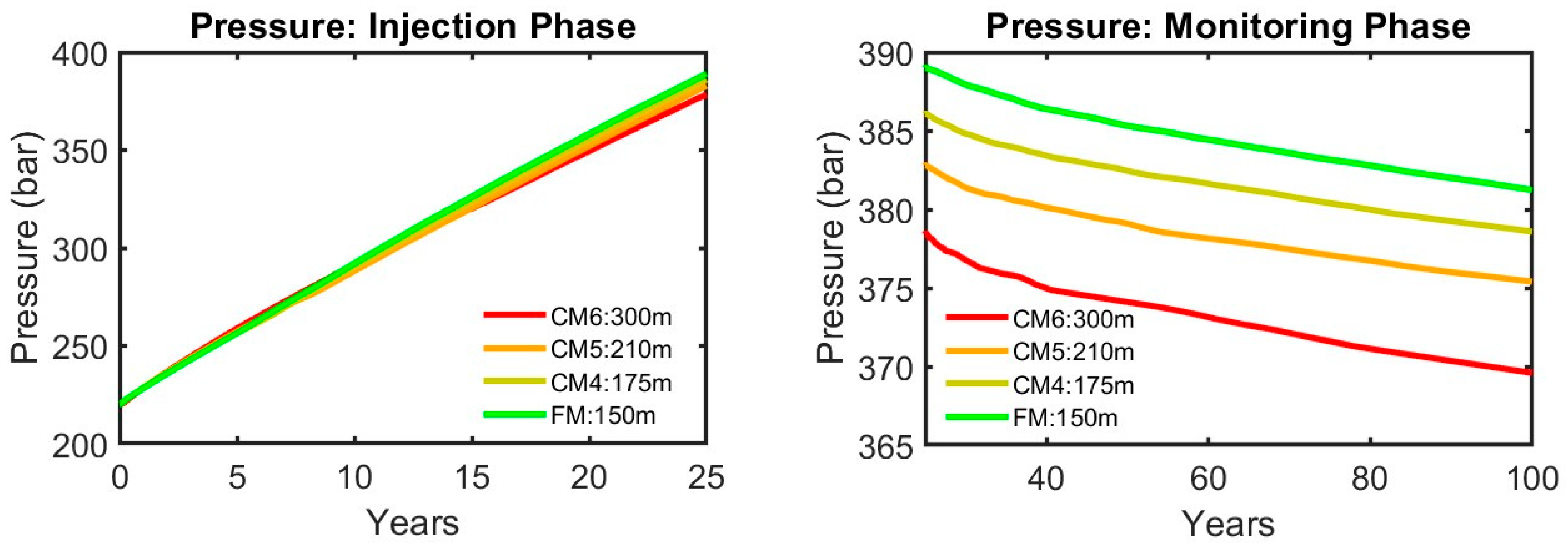
3.3. Lateral Upscaling Impact (X- and Y-Directions)

To evaluate the impact of lateral upscaling (x/y), the same development and injection scenario was used as in Section 3.2, with the injection wells perforated in the lower 50 m of the reservoir. The models tested include Coarse CM4, CM5, and CM6, all with a vertical grid size of 5 m. Additionally, for clarity in tracking plume dynamics, the results are plotted using metric distances rather than grid coordinates. Figure 12 illustrates the effect of varying lateral grid resolutions on the predicted CO₂ plume extent in the top reservoir layer. This layer is critical, as it represents the zone where CO₂ accumulates below the caprock, forming the largest extent of the plume. The analysis was conducted at multiple time steps during both the injection phase (10 and 25 years) and the post-injection monitoring phase (50, 75, and 100 years).

During the injection phase, the overall plume extent is relatively similar across the different lateral grid block sizes, with only a modest loss of detail as the block size increases. The FM model (X/Y: 150 m grid) captures the most detailed and expansive plume, with a mean top layer CO₂ saturation of 0.05 at 10 years and 0.21 at 25 years. This model provides a clear and accurate depiction of early CO₂ migration, showcasing well-defined plume boundaries and a broad spread across the top layer of the reservoir. As we move to coarser grid block sizes, such as CM4 and CM5 (210 m), the plume shape and extent remain largely similar, though there is a slight reduction in the level of detail.

At 10 years, CM4 and CM5 exhibit mean saturations of 0.03 and 0.02, respectively, and by 25 years, their mean saturations increase to 0.19 and 0.16. Despite the reduced detail, the overall plume extent is well-preserved, suggesting that CM4 and CM5 are still capable of providing a reliable prediction during the injection phase. The modest differences observed imply that lateral upscaling to these grid sizes may be acceptable for simulations without significantly compromising accuracy, though some detail is lost. However, the results from CM6 (300 m grid) reveal more substantial limitations. By 10 years, the plume is fully absent, and at 25 years, the plume is underpredicted, with a mean saturation of only 0.07. The CM6 model clearly lacks the resolution needed to capture the plume’s development, indicating that a grid size of 300 m is too coarse for accurately simulating CO₂ migration during the injection phase.

As the system transitions into the monitoring phase, the discrepancies between the models become slightly more pronounced, but overall, the impact of lateral upscaling remains moderate. By 50 years, the FM model continues to offer the most detailed representation of the plume, with a mean saturation of 0.35. The FM’s finer grid resolution allows it to better capture the long-term migration and expansion of the plume as it continues to spread and interact with the top layer. In CM4 (175 m) and CM5 (210 m), the plume’s overall shape and extent remain similar to that of the FM, with lower but still similar mean saturations of 0.33 and 0.30, respectively. The reduction in detail compared to that of the FM is more apparent at this stage, but the overall plume dynamics are still captured reasonably well. This suggests that while CM4 and CM5 grids result in some loss of resolution, they can still be reliably used in simulations, particularly for long-term monitoring, as the differences remain within an acceptable range. However, CM6 (300 m grid) continues to struggle in predicting the plume’s full extent. By 50 years, its mean saturation is only 0.18, and while there is a slight increase by 100 years to 0.23, the plume remains poorly represented compared to the finer grids, making it unsuitable for long-term CO₂ storage simulations, where accurate monitoring is crucial.

Furthermore,

Table 4. Mean absolute error (%) in CO₂ saturation between the FM and coarser models in the lateral directions at key time steps in the injection phase and throughout the entire CCS timeline.

	Injection Phase		Monitoring Phase			Average (Injection Phase and CCS Timeline)
Model	10 Years	25 Years	50 Years	75 Years	100 Years	T1–T25	T1–T100
CM4	37.74%	9.15%	5.26%	4.8%	4.96%	23.44%	12.38%
CM5	56.57%	23.95%	13.75%	13.22%	13.62%	40.26%	24.22%
CM6	100%	65.59%	49%	46.4%	47.57%	82.79%	61.71%

summarizes the mean absolute error (MAE) in CO₂ saturation between the Fine Model (FM) and the coarser laterally upscaled models (CM4, CM5, CM6) across key time steps, covering both the injection and the monitoring phase, as well as the full CCS timeline. While the primary analysis is presented through Figure 12 and the accompanying discussion, Table 4 provides a concise quantitative comparison of model accuracy relative to the FM benchmark. To avoid repetition, we do not further elaborate on the table here, as it reflects the same trends already discussed and visualized.

Overall, the analysis provides a clear picture of how lateral upscaling (x-/y-direction) influences CO₂ plume predictions in the top reservoir layer. While finer grids like the FM (150 m) offer the most detailed representations, coarser models such as CM4 (175 m) and CM5 (210 m) remain effective, showing only minor losses in detail. These coarser grids provide a reliable approximation of plume behavior, making them suitable for both injection and long-term monitoring simulations, with differences that remain within an acceptable margin. Figure 13 further reinforces these findings by illustrating the top-layer mean CO₂ saturation trends over time for each grid resolution. It shows clear convergence among the FM, CM4, and CM5 models, underscoring that these grid resolutions are sufficient to capture the key dynamics of CO₂ migration and storage. The close alignment of CM4 and CM5 with the FM confirms that these models can be adopted with minimal compromise to accuracy, especially for long-term assessments. On the other hand, CM6 (300 m) diverges significantly from the other models. The lower mean saturations and less detailed plume representation in CM6 suggest that this model is inadequate for accurately predicting plume migration and saturation over time. The coarse block size fails to capture the complexities of CO₂ behavior, leading to the underestimation of the plume extent and dynamics. The results indicate that grid convergence is already achieved at the resolutions tested, even for relatively coarser lateral grids (e.g., 175 m). The differences between results from finer and coarser grids are minimal, and further refinement would not provide additional insights. This suggests that the lateral grid resolution is sufficient to accurately represent the spatial distribution and migration dynamics of the CO₂ plume.

In summary, lateral upscaling shows a more moderate impact on CO₂ plume prediction compared to the vertical one. While the CM4 and CM5 grids result in some loss of detail, they still provide acceptable results within a reasonable range. However, CM6, with its very coarse grid resolution, is inadequate for accurate long-term simulations. The selection of grid size must therefore balance computational efficiency with the need for accuracy, particularly when assessing long-term CO₂ storage and migration behavior.

When evaluating the quantitative impact of lateral grid resolution on in situ CO₂ modeling, Figure 14 illustrates the behavior of free and dissolved CO₂ over time, comparing various lateral grid resolutions during both the injection phase and the monitoring phase. These profiles support the understanding on how lateral upscaling influences the CO₂ distribution between its free and dissolved states in the reservoir.

In the free CO₂ profile (top left), all models predict very close results during the injection phase. By year 25, they all converge at around 3.3 Mt of free CO₂, with minimal variation between them. The difference between the FM (150 m) and CM6 (300 m) models is less than 1%, indicating that lateral grid resolution has an insignificant impact on free CO₂ predictions during the injection period. Meanwhile, a more nuanced picture emerges when examining the dissolved CO₂ profile (top right). The dissolved CO₂ profile shows slightly larger differences, though still within a reasonable range. At year 25, the FM (150 m) predicts about 0.40 Mt of dissolved CO₂, whereas CM6 (300 m) predicts a higher value of approximately 0.61 Mt—a difference of 50%. CM4 (175 m) and CM5 (210 m) show results closer to those of the FM; however; it appears that coarser grids tend to slightly overestimate CO₂ dissolution during the injection phase, but the difference remains acceptable for CM4 and CM5. However, CM6 shows signs of divergence from the overall trend overestimating dissolution to a greater degree.

During the post-injection monitoring phase, the free CO₂ profile (bottom left) begins to show more noticeable differences between the models. By year 100, the FM predicts about 3.18 Mt of free CO₂, while CM6 shows a steeper decline, reaching only 2.85 Mt—representing a difference of around 10%. Meanwhile, CM4 and CM5 show free CO₂ values of approximately 3.1 Mt and 3.00 Mt, respectively, reflecting differences in the range of 3% compared to the FM. These results indicate that while lateral grid resolution affects long-term free CO₂ predictions, the impact is relatively minor for CM4 and CM5 but becomes more pronounced for CM6, which deviates significantly from the other models. The dissolved CO₂ profile (bottom right) highlights further divergence in model predictions during the monitoring phase. By year 100, the FM estimates around 0.57 Mt of dissolved CO₂, while CM6 predicts about 0.81 Mt, reflecting a 40% increase. CM4 and CM5 predict dissolved CO₂ values of around 0.62 Mt and 0.70 Mt, respectively—differences in the range of 10% from the FM. This suggests that while CM4 and CM5 remain reasonably close to the FM in terms of capturing CO₂ dissolution trends, CM6 continues to overestimate dissolution, diverging significantly from the finer grid models.

The analysis highlights that lateral grid resolution has a relatively minor impact on free CO₂ predictions during the injection phase, with differences of less than 1% between the finest grid (FM: 150 m) and the coarsest grid (CM6: 300 m). However, in the dissolved CO₂ profile during the injection phase, coarser grids like CM6 show a more significant overestimation, with differences of up to 50% compared to the FM. During the monitoring phase, the divergence becomes more pronounced, particularly for CM6. The free CO₂ differences between the FM and CM6 increase to around 10%, while dissolved CO₂ differences reach up to 40%. CM4 and CM5 remain close to the FM, with differences of 3–5% for free CO₂ and 10–20% for dissolved CO₂, making them reliable alternatives. In conclusion, CM4 and CM5 offer acceptable results, with resolutions that could be adopted for both injection and monitoring phases, while CM6 introduces considerable errors and should be avoided in scenarios where precision is required.

Figure 15 illustrates the pressure evolution in the reservoir during both the injection phase (left) and the monitoring phase (right), comparing different lateral grid resolutions.

During the injection phase, the pressure buildup across all models is nearly identical, with pressure steadily increasing from around 220 bar to 395 bar by year 25. The differences between the grid resolutions are minimal, with less than a 3% variation between the FM and CM6, which is consistent with the earlier observation that free CO₂ predictions are nearly identical during this phase. This indicates that lateral grid resolution has a negligible impact on pressure evolution during the injection period, as the majority of CO₂ remains in the free phase and uniformly drives pressure increases in all models. In the monitoring phase, the pressure decline begins to show a slight increase in the differences between the models, mirroring the trends observed in the free CO₂ profile. The FM (150 m) predicts the most gradual pressure decline, with pressure decreasing from about 390 bar to 380 bar over the course of 75 years. CM4 and CM5 also show similar pressure trends, with slight but acceptable differences, reflecting the relatively modest impact of lateral grid resolution on long-term pressure predictions. However, CM6 (300 m) exhibits a much steeper pressure decline, with pressure falling to around 370 bar by year 100—approximately 10 bar lower than the FM. This 2.6% difference in pressure is directly correlated with the 10% lower free CO₂ levels predicted by CM6 during the same time frame. The more rapid reduction in free CO₂ leads to a faster loss of pressure, as free CO₂ is the primary source of compressibility in the system.

Overall, the analysis of free CO₂, dissolved CO₂, and pressure profiles shows that coarser grid models tend to exhibit certain biases in their predictions. While the finest grid (FM) offers the most precise predictions, CM4 and CM5 grid resolutions, up to 200 m in moderately heterogeneous reservoirs, can be considered reliable alternatives, with only minor overestimations of CO₂ dissolution and minor underestimations of pressure. However, for highly heterogeneous reservoirs, a 150 m grid resolution would be a safer option to ensure more accurate predictions.

4. Discussion

The selection of a simulation framework for CO₂ storage in saline aquifers is not merely a technical decision but also one that carries substantial regulatory, economic, and operational consequences. As CCS projects evolve from conceptual design to full-scale deployment and post-injection monitoring, the modeling tools employed must reflect both the physical realism required by the problem and the confidence levels acceptable to stakeholders and regulators.

In early-stage development—particularly in frontier basins where data is sparse and decisions must often be made under uncertainty—the Black Oil Model (BoM) provides a pragmatic entry point. Its relative simplicity, computational efficiency, and conservative estimates of CO₂ plume extent and pressure buildup make it valuable for bounding scenarios and defining initial monitoring zones. Importantly, the BoM implementation used in this study builds on an Equation of state (EOS)-tuned framework, where dissolution is not strictly neglected but rather captured indirectly through calibrated pseudo-components. This adaptation allows it to approximate key storage behaviors while remaining tractable for large-scale or uncertainty-based analyses such as Design of Experiment (DoE) or sensitivity runs.

Meanwhile, to avoid introducing bias by selecting a single “reference” simulator, this study adopts a multi-model benchmarking strategy, comparing the BoM with compositional simulators incorporating various EOS-based solubility models. This approach reflects the current lack of field-validated ground truth and highlights the importance of cross-validation in model evaluation. Notably, the BoM consistently aligns closely with all benchmarked models, even without defining a single reference, reinforcing its credibility for early- to mid-stage CCS assessments. While this lends confidence to its predictive performance, particularly for large-scale sensitivity studies, we acknowledge that definitive validation against laboratory or field data remains essential. Future work should therefore prioritize empirical comparisons to further constrain uncertainties and refine the model’s long-term reliability.

Furthermore, the BoM’s utility diminishes when the simulation must address regulatory processes involving crediting, mass accounting, or liability transfer. These later stages require detailed tracking of solubility trapping, impurity effects, and phase evolution—all of which demand a detailed representation of phase behavior, and therefore a compositional approach. Tools like CMG-GEM, governed by EOS formulations and capable of handling complex phase behavior (to the extent that the EoS and brine fugacity models utilized are accurate), become indispensable under such conditions. Furthermore, compositional simulations are essential when non-condensable gases or acid components are present in the injected CO₂ stream, which substantially alters phase behavior and storage performance. While EU regulations mandate that the CO₂ stream be “overwhelmingly” composed of CO₂—with only minor, justified impurities allowed for monitoring purposes—the mere presence of these components necessitates more sophisticated modeling.

From a regulatory standpoint, a hybrid or bracketing approach—using both BoM and compositional simulations—may offer the most robust pathway. The BoM can define conservative envelopes and screen scenarios, while compositional models refine understanding for permitting, optimization, and post-injection monitoring.

To clarify the respective strengths and limitations of these modeling paradigms,

Table 5. Comparison of the Black Oil Model vs. compositional models in CO₂ storage simulation contexts.

Criteria	Black Oil Model (BoM)	Compositional Models (e.g., GEM)
CO2 phase treatment	CO2 treated as pseudo-oil or pseudo-gas; simplified representation	Full thermodynamic equilibrium between phases using EoS
Dissolution handling	Indirect (via tuning/solubility model); no explicit mass transfer between phases	Explicit solubility trapping governed by EoS & equilibrium constraints
Impurity effects	Cannot capture non-ideal behavior from impurities unless thermodynamic model is tuned	Captures multi-component, non-ideal phase behavior if EoS is appropriately tuned
Computational cost	Low; suitable for large-scale screening runs and prospecting tasks	High; especially with multiple components and fine resolution
Data requirements	Moderate; fewer fluid-specific inputs	High; requires PVT data, EOS tuning, and phase-behavior characterization
Regulatory use—early stage	Acceptable, with caveats and sensitivity analyses (e.g., DoE)	Preferred but not always required (case specific)
Regulatory use—liability transfer	Insufficient for mass accounting, dissolution tracking, and MRV compliance	Essential for regulatory compliance and long-term liability transfer

summarizes their performance across key simulation and regulatory dimensions.

Furthermore, it is worth noting that the solubility model integrated in this work has been experimentally validated up to 600 bar and 300 °C, extending its technical applicability beyond typical carbon storage conditions. While this broad thermodynamic envelope allows for potential use in CO₂ Plume Geothermal (CPG) systems or other hybrid storage–utilization concepts, the present study focuses on conditions most representative of saline aquifer storage. In practice, CCS sites are intentionally selected to operate just above the CO₂ critical point (31.1 °C and 73.8 bar), typically within 35–120 °C and 300–350 bar, to ensure supercritical behavior and maximize storage efficiency. Although the current BoM parameterization is consistent with these conditions, the same modeling framework—while promising—remains to be rigorously validated and verified for CPG applications or geothermal–CCS hybrid systems, where additional coupled thermal and flow processes may become dominant.

In addition, it is important to acknowledge that the current modeling framework assumes a two-phase system (aqueous brine and CO₂) and neglects the vaporization of water into the CO₂-rich phase. This simplification is justified under the typical temperature and pressure conditions of most CO₂ storage reservoirs, where water vaporization is minimal and has a negligible impact on overall mass balance or storage efficiency. However, under certain scenarios—such as near wellbore regions, shallow formations, or higher-temperature regimes—the vaporization of brine and subsequent effects like salt precipitation and dry-out may become non-negligible. These processes can affect local injectivity and porosity, and their modeling may require a fully compositional approach with thermophysical coupling. Such extensions are especially relevant in hybrid CO₂ storage–utilization concepts like CPG, where thermal gradients and dry CO₂ injection are more pronounced. While these effects are outside the scope of the current study and were not assessed, they represent important considerations for detailed site-specific assessments or late-stage regulatory evaluations.

Moreover, the brine properties in this study are modeled using the Rowe & Chou (1970) [38] and Kestin et al. (1981) [39] correlations, which remain widely used in reservoir simulation due to their simplicity and reasonable accuracy within moderate salinity (<150,000 ppm) and temperature (<150 °C) ranges. However, under more extreme thermodynamic conditions—such as hypersaline environments or high-temperature systems relevant to CO₂ Plume Geothermal (CPG) applications—these empirical models may become less reliable. In such cases, more recent correlations or advanced thermodynamic frameworks like Pitzer or eNRTL could enhance the accuracy of brine property predictions. For future work focused on geothermal–CCS hybrids or high-fidelity site-specific modeling, the adoption of these models is recommended to ensure better physical consistency in fluid property estimations.

It is important to note that while the BoM employed in this study does not explicitly account for capillary pressure–saturation relationships, it indirectly captures the effects of capillary trapping using residual gas saturation (Sgr) and relative permeability hysteresis. These parameters effectively approximate the immobilization of CO₂ by capillary forces, offering a simplified but practical representation of capillary trapping, especially when laboratory core-flood data or field estimates are not available. This approach is consistent with common practices for early-stage screening and sector modeling, where more detailed capillary pressure functions may not be necessary. However, it is critical to acknowledge that capillary trapping is a dynamic process driven by pore-scale displacement and hysteresis effects. Such models would be particularly beneficial during post-injection phases, where redistribution and residual trapping are more significant. Thus, while our BoM-based approach is shown to be suitable for initial CCS appraisal, it should be recognized that for more precise assessments, particularly those aimed at long-term storage security, higher-fidelity models that integrate capillary pressure and saturation relationships or even pore-scale simulations may be necessary.

5. Conclusions

Climate change remains one of the defining challenges of our era, demanding deep and sustained reductions in greenhouse gas emissions to meet global climate targets. Among the available mitigation strategies, Carbon Capture and Storage (CCS) stands out as a critical pillar—particularly for decarbonizing hard-to-abate industrial sectors such as cement, steel, and refining. CCS enables the permanent storage of CO₂ in deep geological formations, offering a scalable pathway to reduce emissions from existing infrastructure and to facilitate negative emission strategies.

However, the success of CCS depends heavily on the reliability and efficiency of subsurface modeling tools used to predict CO₂ behavior under a range of geological and operational conditions. In this context, the present study contributes to two key areas: first, by validating the Black Oil Model (BoM) as a streamlined yet robust alternative to fully compositional simulators; and second, by evaluating the sensitivity of CCS model performance to spatial grid resolution—a factor with direct implications for reservoir characterization, monitoring strategy, risk assessment, and regulatory compliance.

To assess the viability of the BoM, its results were benchmarked against three well-established compositional simulators—Eclipse E300, CMG-GEM, and TNavigator—using an industry-representative, heterogeneous 3D saline aquifer model. The BoM was found to reliably reproduce CO₂ plume migration, shape, and saturation profiles, with mean deviations across all compositional models of 2.6% during the injection phase and 4.6% during post-closure monitoring, and an overall average deviation of 3.8% along the entire CCS project period. Free gas predictions at the end of the injection period (25 years) deviated by less than 0.6% relative to Eclipse and TNavigator, and by 5.4% compared to CMG-GEM. At the end of the monitoring period (100 years), deviations remained modest—around 2.5% for Eclipse and TNavigator, and 7.9% for CMG-GEM.

Regarding dissolved CO₂, the BoM aligned well with Eclipse and TNavigator, with deviations of 2.5% at the end of injection and 9.4% at the end of monitoring. However, it showed significantly higher deviations from CMG-GEM (38.1% and 34.1%, respectively), attributable to GEM’s use of Henry’s Law for modeling CO₂ solubility. Pressure predictions across all simulators showed strong agreement, with deviations consistently below 1.2%.

These results confirm the BoM as a computationally efficient and reliable alternative for CO₂ storage simulation in saline aquifers, particularly during early-phase feasibility studies where rapid, large-scale assessments are required without compromising accuracy.

The study also rigorously investigated the impact of spatial grid resolution, a critical factor for accurately simulating plume dynamics. Vertical resolution proved especially influential during the post-injection phase, with 2 m grids capturing plume shape, gravitational segregation, and dissolution behavior effectively. In contrast, coarser grids led to significant underestimation of plume extent near the reservoir top, with mean CO₂ saturation deviations during the monitoring period reaching 15% for 5 m, 40% for 10 m, 73% for 25 m, and 86% for 50 m grids. Such discrepancies could substantially impact the design of monitoring plans, corrective action strategies, and long-term liability frameworks.

Lateral resolution had greater influence during the injection phase, affecting injection strategy, storage efficiency, and overall site performance. A lateral grid size of 150 m was found to balance accuracy with computational efficiency, while 200 m remained acceptable in scenarios with limited computational resources. Beyond this, coarser grids failed to capture the in situ behavior of CO₂ accurately, particularly during injection.

Based on these findings, the study recommends a vertical grid resolution of 2 m or finer, and a lateral resolution in the range of 150–200 m for modeling CO₂ storage in moderately heterogeneous saline aquifers. Nevertheless, future work should assess the impact of local grid refinement near critical features—such as wellbores, caprocks, and high-permeability pathways—where detailed flow dynamics must be resolved, especially for regulatory compliance and risk-informed monitoring.

The applicability of these guidelines, while robust for reservoirs with Gaussian-distributed heterogeneity, should be extended to more complex geological settings. These include fractured reservoirs with discrete flow conduits, formations with strong vertical heterogeneity or barriers, and those with significant anisotropy (Kv/Kh > 10:1) or non-Gaussian heterogeneity, such as channelized systems or diagenetically altered zones. In such cases, finer vertical grids (≤1 m), discrete feature modeling, or multiscale simulation approaches may be required.

Additionally, the selection of the BoM must be informed by the CO₂ stream composition. In this study, the BoM was tuned to a pure CO₂ stream using a customized Equation of State (EoS). However, for injection streams containing impurities such as N₂, O₂, or SO₂, compositional simulators may be necessary to capture the multiphase and reactive behavior of these mixtures. Alternatively, further research could adapt the BoM by tuning its EoS to account for such impurities. These distinctions affect CO₂ solubility, phase behavior, and reservoir pressure responses—ultimately impacting well design, monitoring strategy, and regulatory reporting.

In conclusion, this study affirms the Black Oil Model as a viable and efficient tool for simulating CO₂ storage in saline aquifers and provides practical guidance on optimal grid resolution. However, the findings also highlight the need for site-specific adaptations—whether through compositional modeling, localized grid refinement, or hybrid approaches—to ensure technically robust and regulatory-compliant CCS deployment across diverse geological environments.

References

1. International Energy Agency (IEA). Global Energy Review: CO2 Emissions in 2022. 2022. Available online: https://iea.blob.core.windows.net/assets/3c8fa115-35c4-4474-b237-1b00424c8844/CO2Emissionsin2022.pdf (accessed on 15 November 2024).
2. International Energy Agency (IEA) and Cement Sustainability Initiative (CSI). Technology Roadmap: Low-Carbon Transition in the Cement Industry. 2018. Available online: https://iea.blob.core.windows.net/assets/cbaa3da1-fd61-4c2a-8719-31538f59b54f/TechnologyRoadmapLowCarbonTransitionintheCementIndustry.pdf (accessed on 15 November 2024).
3. Intergovernmental Panel on Climate Change (IPCC). Sixth Assessment Report (AR6)—Working Group III: Mitigation of Climate Change. 2022. Available online: https://www.ipcc.ch/report/ar6/wg3/downloads/report/IPCC_AR6_WGIII_FullReport.pdf (accessed on 15 November 2024).
4. European Commission. A New Circular Economy Action Plan: For a Cleaner and More Competitive Europe. 2020. Available online: https://eur-lex.europa.eu/legal-content/EN/TXT/HTML/?uri=CELEX:52020DC0098 (accessed on 15 November 2024).
5. Global CCS Institute. Global Status of CCS 2021. 2021. Available online: https://www.globalccsinstitute.com/wp-content/uploads/2023/01/Global-Status-of-CCS-2021-Global-CCS-Institute-1121-1-1.pdf (accessed on 15 November 2024).
6. Benson, S.M.; Cole, D.R. CO2 Sequestration in Deep Sedimentary Formations. Elements 2008, 4, 325–331. [Google Scholar] [CrossRef]
7. Ji, X.; Zhu, C. CO2 Storage in Deep Saline Aquifers. In Novel Materials for Carbon Dioxide Mitigation Technology; Elsevier: Amsterdam, The Netherlands, 2015; pp. 299–332. [Google Scholar] [CrossRef]
8. Hannis, S.; Lu, J.; Chadwick, A.; Hovorka, S.; Kirk, K.; Romanak, K.; Pearce, J. CO2 Storage in Depleted or Depleting Oil and Gas Fields: What can We Learn from Existing Projects? Energy Procedia 2017, 114, 5680–5690. [Google Scholar] [CrossRef]
9. Gassara, O.; Estublier, A.; Garcia, B.; Noirez, S.; Cerepi, A.; Loisy, C.; Le Roux, O.; Petit, A.; Rossi, L.; Kennedy, S.; et al. The Aquifer-CO2Leak project: Numerical modeling for the design of a CO2 injection experiment in the saturated zone of the Saint-Emilion (France) site. Int. J. Greenh. Gas Control. 2021, 104, 103196. [Google Scholar] [CrossRef]
10. Ismail, I.; Gaganis, V. Carbon Capture, Utilization, and Storage in Saline Aquifers: Subsurface Policies, Development Plans, Well Control Strategies and Optimization Approaches—A Review. Clean Technol. 2023, 5, 609–637. [Google Scholar] [CrossRef]
11. Pruess, K.; García, J.; Kovscek, T.; Oldenburg, C.; Rutqvist, J.; Steefel, C.; Xu, T. Code intercomparison builds confidence in numerical simulation models for geologic disposal of CO2. Energy 2004, 29, 1431–1444. [Google Scholar] [CrossRef]
12. Class, H.; Ebigbo, A.; Helmig, R.; Dahle, H.K.; Nordbotten, J.M.; Celia, M.A.; Audigane, P.; Darcis, M.; Ennis-King, J.; Fan, Y.; et al. A benchmark study on problems related to CO2 storage in geologic formations. Comput. Geosci. 2009, 13, 409–434. [Google Scholar] [CrossRef]
13. Ismail, I.; Fotias, S.P.; Avgoulas, D.; Gaganis, V. Integrated Black Oil Modeling for Efficient Simulation and Optimization of Carbon Storage in Saline Aquifers. Energies 2024, 17, 1914. [Google Scholar] [CrossRef]
14. Aziz, K.; Settari, A. Petroleum Reservoir Simulation; Elseviers: Amsterdam, The Netherlands, 1979. [Google Scholar]
15. Peaceman, D.W. Fundamentals of Numerical Reservoir Simulation; Elsevier: Amsterdam, The Netherlands, 1977. [Google Scholar]
16. Blair, L.M.; Quinn, J.A. Measurement of Small Density Differences: Solutions of Slightly Soluble Gases. Rev. Sci. Instrum. 1968, 39, 75–77. [Google Scholar] [CrossRef]
17. Sayegh, S.G.; Najman, J. Phase behavior measurements of CO2-SO2-brine mixtures. Can. J. Chem. Eng. 1987, 65, 314–320. [Google Scholar] [CrossRef]
18. Ennis-King, J.; Paterson, L. Role of Convective Mixing in the Long-Term Storage of Carbon Dioxide in Deep Saline Formations. In Proceedings of the SPE Annual Technical Conference and Exhibition, Denver, CO, USA, 5–8 October 2003. [Google Scholar] [CrossRef]
19. Hassanzadeh, H.; Pooladi-Darvish, M.; Keith, D.W. Modelling of Convective Mixing in CO2 Storage. J. Can. Pet. Technol. 2005, 44, PETSOC-05-10-04. [Google Scholar] [CrossRef]
20. Coats, K.H. An Equation of State Compositional Model. Soc. Pet. Eng. J. 1980, 20, 363–376. [Google Scholar] [CrossRef]
21. Young, L.C.; Stephenson, R.E. A Generalized Compositional Approach for Reservoir Simulation. Soc. Pet. Eng. J. 1983, 23, 727–742. [Google Scholar] [CrossRef]
22. Yang, Z.-L.; Yu, H.-Y.; Chen, Z.-W.; Cheng, S.-Q.; Su, J.-Z. A compositional model for CO2 flooding including CO2 equilibria between water and oil using the Peng–Robinson equation of state with the Wong–Sandler mixing rule. Pet Sci. 2019, 16, 874–889. [Google Scholar] [CrossRef]
23. Li, H.; Durlofsky, L.J. Ensemble level upscaling for compositional flow simulation. Comput. Geosci. 2016, 20, 525–540. [Google Scholar] [CrossRef]
24. He, C.; Durlofsky, L.J. Structured flow-based gridding and upscaling for modeling subsurface flow. Adv. Water Resour. 2006, 29, 1876–1892. [Google Scholar] [CrossRef]
25. Ringrose, P.; Bentley, M. Reservoir Model Design; Springer: Cham, Switzerland, 2021. [Google Scholar] [CrossRef]
26. Pickup, G.E.; Kiatsakulphan, M.; Mills, J.R. Analysis of Grid Resolution for Simulations of CO2 Storage in Deep Saline Aquifers. In Proceedings of the ECMOR XII—12th European Conference on the Mathematics of Oil Recovery, Oxford, UK, 6–9 September 2010. [Google Scholar] [CrossRef]
27. Rabinovich, A.; Itthisawatpan, K.; Durlofsky, L.J. Upscaling of CO2 injection into brine with capillary heterogeneity effects. J. Pet. Sci. Eng. 2015, 134, 60–75. [Google Scholar] [CrossRef]
28. Ismail, I.; Fotias, S.P.; Tartaras, E.; Stefatos, A.; Gaganis, V. Impact of Grid Resolution on Accuracy of In-Situ CO2 Modeling for Improved CCS Project Design and Implementation. In Proceedings of the Mediterranean Offshore Conference, Alexandria, Egypt, 20–22 October 2024. [Google Scholar] [CrossRef]
29. Mo, S.; Akervoll, I. Modeling Long-Term CO2 Storage in Aquifer with a Black-Oil Reservoir Simulator. In Proceedings of the SPE/EPA/DOE Exploration and Production Environmental Conference, Galveston, TX, USA, 7–9 March 2005. [Google Scholar] [CrossRef]
30. Hassanzadeh, H.; Pooladi-Darvish, M.; Elsharkawy, A.M.; Keith, D.W.; Leonenko, Y. Predicting PVT data for CO2–brine mixtures for black-oil simulation of CO2 geological storage. Int. J. Greenh. Gas Control. 2008, 2, 65–77. [Google Scholar] [CrossRef]
31. Pour, S.S.; Pickup, G.E.; Mackay, E.J.; Heinemann, N. Flow Simulation of CO2 Storage in Saline Aquifers Using Black Oil Simulator. In Proceedings of the Carbon Management Technology Conference, Orlando, FL, USA, 7–9 February 2012. [Google Scholar] [CrossRef]
32. Spycher, N.; Pruess, K. CO2-H2O mixtures in the geological sequestration of CO2. II. Partitioning in chloride brines at 12–100 °C and up to 600 bar. Geochim. Cosmochim Acta 2005, 69, 3309–3320. [Google Scholar] [CrossRef]
33. Duan, Z.; Sun, R. An improved model calculating CO2 solubility in pure water and aqueous NaCl solutions from 273 to 533 K and from 0 to 2000 bar. Chem. Geol. 2003, 193, 257–271. [Google Scholar] [CrossRef]
34. Kumar, A. A Simulation Study of Carbon Sequestration in Deep Saline Aquifers. Master’s Thesis, The University of Texas at Austin, Austin, TX, USA, 2004. [Google Scholar]
35. Spycher, N.; Pruess, K.; Ennis-King, J. CO2-H2O mixtures in the geological sequestration of CO2. I. Assessment and calculation of mutual solubilities from 12 to 100 °C and up to 600 bar. Geochim. Cosmochim. Acta 2003, 67, 3015–3031. [Google Scholar] [CrossRef]
36. Spycher, N.; Pruess, K. A Phase-Partitioning Model for CO2–Brine Mixtures at Elevated Temperatures and Pressures: Application to CO2-Enhanced Geothermal Systems. Transp. Porous Media 2010, 82, 173–196. [Google Scholar] [CrossRef]
37. Duan, Z.; Sun, R.; Zhu, C.; Chou, I.-M. An improved model for the calculation of CO2 solubility in aqueous solutions containing Na+, K+, Ca2+, Mg2+, Cl, and SO42−. Mar. Chem. 2006, 98, 131–139. [Google Scholar] [CrossRef]
38. Rowe, A.M.; Chou, J.C.S. Pressure-volume-temperature-concentration relation of aqueous sodium chloride solutions. J. Chem. Eng. Data 1970, 15, 61–66. [Google Scholar] [CrossRef]
39. Kestin, J.; Khalifa, H.E.; Correics, R.J. Tables of the Dynamic and Kinematic Viscosity of Aqueous NaCl Solution in the Temperature Range 20-150 C and the Pressure Range 0.1–35 MPa. J. Phys. Chem. Ref. Data 1981, 10, 71–88. [Google Scholar] [CrossRef]
Figure 1. Reservoir properties and distribution.
Processes 13 01901 g001
Figure 2. PVT dataset adopted in the BoM simulation (a): Brine formation volume factor (FVF) and solubility, (b): Brine viscosity, (c): CO2 FVF, and (d): CO2 viscosity.
Processes 13 01901 g002
Figure 3. Well locations (I1 and I2): (a) 3D view and (b) 2D view (top layer).
Processes 13 01901 g003
Figure 4. CO2 saturation in the top layer at different time steps (injection: 10, 25 years & Monitoring: 50–100 years) for all model simulations.
Processes 13 01901 g004
Figure 5. Free CO2 profiles across the injection and post-closure monitoring phases for all simulation models.
Processes 13 01901 g005
Figure 6. Dissolved CO2 profiles across the injection and post-closure monitoring phases for all simulation models.
Processes 13 01901 g006
Figure 7. Field pressure profile across the injection and post-closure monitoring phases for all simulation models.
Processes 13 01901 g007
Figure 8. Comparison of CO2 plume extent and shape at the top layer across different vertical grid resolutions at various time steps.
Processes 13 01901 g008
Figure 9. Mean saturation comparison across different years for various vertical grid resolutions.
Processes 13 01901 g009
Figure 10. Profiles of free and dissolved CO2 over time during the operation phase and the monitoring phase, analyzed across different vertical grid resolution models.
Processes 13 01901 g010
Figure 11. Field pressure evolution during both the operation phase and the monitoring phase across different vertical resolution models.
Processes 13 01901 g011
Figure 12. Comparison of CO2 plume extent and shape at the top layer across different lateral grid resolutions at various time steps.
Processes 13 01901 g012
Figure 13. Mean saturation comparison across different years for various lateral grid resolutions.
Processes 13 01901 g013
Figure 14. Profiles of free and dissolved CO2 over time during the operation phase and the monitoring phase, analyzed across different lateral grid resolutions.
Processes 13 01901 g014
Figure 15. Field pressure evolution during both the operation phase and the monitoring phase across different lateral resolution models.
Processes 13 01901 g015