Research on Self-Healing Distribution Network Operation Optimization Method Considering Carbon Emission Reduction

Abstract

To improve the consumption rate of distributed energy and enhance the self-healing performance of distribution networks, this paper proposes a distribution network optimization method considering carbon emissions and dynamic reconfiguration. Firstly, various measures such as dynamic reconfiguration and distributed energy scheduling are used in upper-level optimization to reduce the network loss and solar curtailment cost of the system and to realize the optimal economic operation of the distribution network. Secondly, based on carbon emission flow theory in lower-level optimization, a low-carbon demand response model with a dynamic carbon emission factor as the guiding signal is established to promote carbon emission reduction on the user side. Then, the second-order cone planning and improved dung beetle optimization algorithm are used to solve the model. Finally, it is verified on the test system that the method can effectively reduce the risk of voltage overruns and enhance the low-carbonization and economy of distribution network operation.

1. Introduction

As the installed capacity of distributed energy sources such as wind power and photovoltaics (PV) gradually increases, there is a great challenge to the safe and stable operation of distribution networks, and traditional control methods are no longer applicable [1,2,3,4]. The concept of active distribution networks (ADNs) provides a new way to operate and control distribution networks [5,6]. ADNs have a flexible network structure, utilize distributed energy, demand-side response, energy storage systems (ESSs), and other controllable resources, and are able to effectively cope with the impact of distributed energy grid connection [7,8,9].

A large number of scholars have studied the optimized operation of ADNs. In [10], the temporal and spatial distribution characteristics of EVs were considered to accurately predict EV loads, based on which a joint optimization model considering the dynamic reconfiguration of ADNs was established which effectively reduces system operation cost and voltage fluctuation. In [11], the distributed accelerated alternating direction multiplier method was used for zonal optimization of the scheduling of an ADN containing distributed energy, and the results show that the method can effectively promote local consumption of distributed energy and reduce the impact of grid connections on higher-level grids. In [12], a coordinated optimization strategy for an ADN based on model predictive control was proposed which could improve system economy and voltage quality. The above studies focused on the economy of ADN operation and lacked analysis of the low carbonization of systems.

Power systems are one of the main sources of carbon emissions, and their low carbonization has received widespread attention. In [13,14], a carbon trading mechanism was utilized to realize the economy and low carbonization of the power system. In [15], a total carbon emission constraint was added to the generation units output problem to realize the distributed low-carbonization scheduling of the system. In [16], considering the operation characteristics of carbon capture power plants, wind power, thermal power, nuclear power, and carbon capture power plants were jointly optimized. The above studies mainly promoted carbon emission reduction by means of carbon quotas as well as optimal scheduling, without considering the impact of user electricity consumption behavior on carbon emission reduction. Carbon emission flow theory can accurately describe the carbon emissions of all links in a power system, providing a theoretical basis for guiding users to directly participate in carbon emission reduction [17,18,19]. In [20], a new mechanism of demand response of the power system with dynamic carbon emission factor as the guiding signal was proposed. In [21,22,23], different types of loads were refined and categorized, and matching demand response strategies were formulated, but active power loss generated in the transmission process as well as the node voltage safety range were neglected. Performance comparison of different methods is shown in

Table 1. Performance comparison of different methods.

	Low-Carbon Characteristics	Economic Efficiency	Demand Response and Dynamic Reconfiguration
[15]	Low	Low	×
[16]	Medium	Medium	×
[20]	High	Medium	×
This paper	High	High	√

.

Based on previous research, this paper analyzes the characteristics of carbon emission flows in ADNs containing distributed energy and proposes a novel optimization strategy. The upper-level optimization model is the optimal economic scheduling model for ADNs, and combines dynamic reconfiguration of ADNs with active management measures of distributed energy to achieve the lowest network loss and cost of solar curtailment with consideration of the security constraints of ADNs such as line current, voltage magnitude, etc. The lower-level optimization model calculates carbon emission flow based on the optimized power flow result of the upper-level model and adjusts the system load curve with the optimization objective of minimizing the scheduling cost and total carbon emission so as to enhance the promotion effect of the user-side response on carbon emission reduction. The second-order cone planning and improved dung beetle optimizer (IDBO) algorithm are used to solve the above model [24]. Simulations based on the improved IEEE 33 node system are conducted to verify the economy and low carbonization performance of the proposed method.

2. Demand Response Modeling Considering Carbon Emissions

The traditional price-based demand response generally has peak and valley times of price based on load height, and with the increasing penetration of PV in ADNs the system share of PV power generation at different moments is different, resulting in the carbon emissions of distribution networks showing temporal variability. Therefore, based on the dynamic carbon emission factor (DCEF) [25], this paper divides the moments of high-carbon, flat-carbon, and low-carbon electricity consumption, establishes an elastic demand response model, guides users to adjust their electricity consumption behavior, changes the load distribution of the ADN, promotes the consumption of renewable energy, and reduces system carbon emissions.

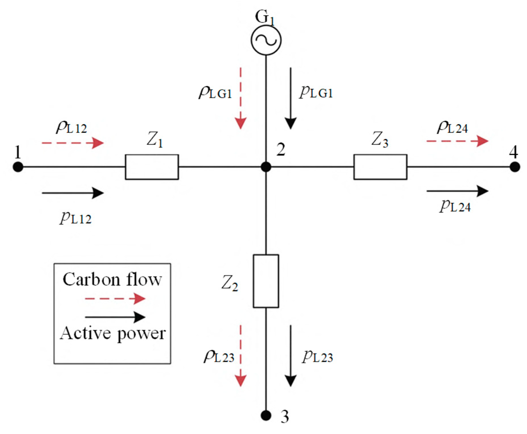
2.1. Carbon Emission Flow of ADN

The carbon emission flow of a power system is a virtual network flow that depends on the system trend and follows the trend in the network. In this paper, we take the ADN shown in Figure 1 as an example to analyze the distribution characteristics of carbon emission flow in an ADN.

According to the principle of shared proportionality [26], in any branch flow out of a node, there exists a component of the branch flow into the node, and thus the carbon flow rate of a branch flow out of the node shall be the sum of the contributions of all the branches flowing into the node and the carbon flow rate of the outgoing branch. Therefore, the carbon flow density of the branch 24 is

$${\rho }_{\mathrm{L}24}={\displaystyle \frac{{{\displaystyle \sum }}_{i\in {\xi }^{+}}{P}_{\mathrm{L}24}\frac{P_{\mathrm{L}i}}{{{\displaystyle \sum }}_{s\in {\xi }^{+}}{P}_{\mathrm{L}s}}{\rho }_{\mathrm{L}i}}{P_{\mathrm{L}2}}}={\displaystyle \frac{{{\displaystyle \sum }}_{i\in {\xi }^{+}}{P}_{\mathrm{L}}{\rho }_{\mathrm{L}i}}{{{\displaystyle \sum }}_{s\in {\xi }^{+}}{P}_{\mathrm{L}s}}}={\displaystyle \frac{{{\displaystyle \sum }}_{s\in {\xi }^{+}}{L}_{\mathrm{L}s}^{\mathrm{CEF}}}{{{\displaystyle \sum }}_{s\in {\xi }^{+}}{P}_{\mathrm{L}s}}}=w_j=w_2$$

(1)

where ${\xi }^{+}$ is the set of all branches with active power flowing into node $j$; ${\rho }_{\mathrm{L}i}$ is the carbon flow density of the branch $i$, whose value is the ratio of the carbon flow rate $L_{\mathrm{L}s}^{\mathrm{CEF}}$ of the branch to the active power $P_{\mathrm{Ls}}$; and $w_j$ is the carbon potential of node $j$.

From (1), the carbon flow density of the branch of the outgoing current is equal to the carbon potential of the upstream node of that branch. Distribution networks generally do not have circulating power, so for passive distribution networks, the injected power of any node is only provided by the unique upstream node of the network; in this case, the carbon potentials of all nodes are kept the same and are equal to the carbon potentials of the upstream nodes. When distributed power is connected in the ADN, the distributed power will affect the carbon potential of the node where it is located, and even the upstream node. Therefore, the carbon flow distribution of the whole ADN can be calculated when the current distribution of the system, the network structure and the carbon potential of the upstream node are known.

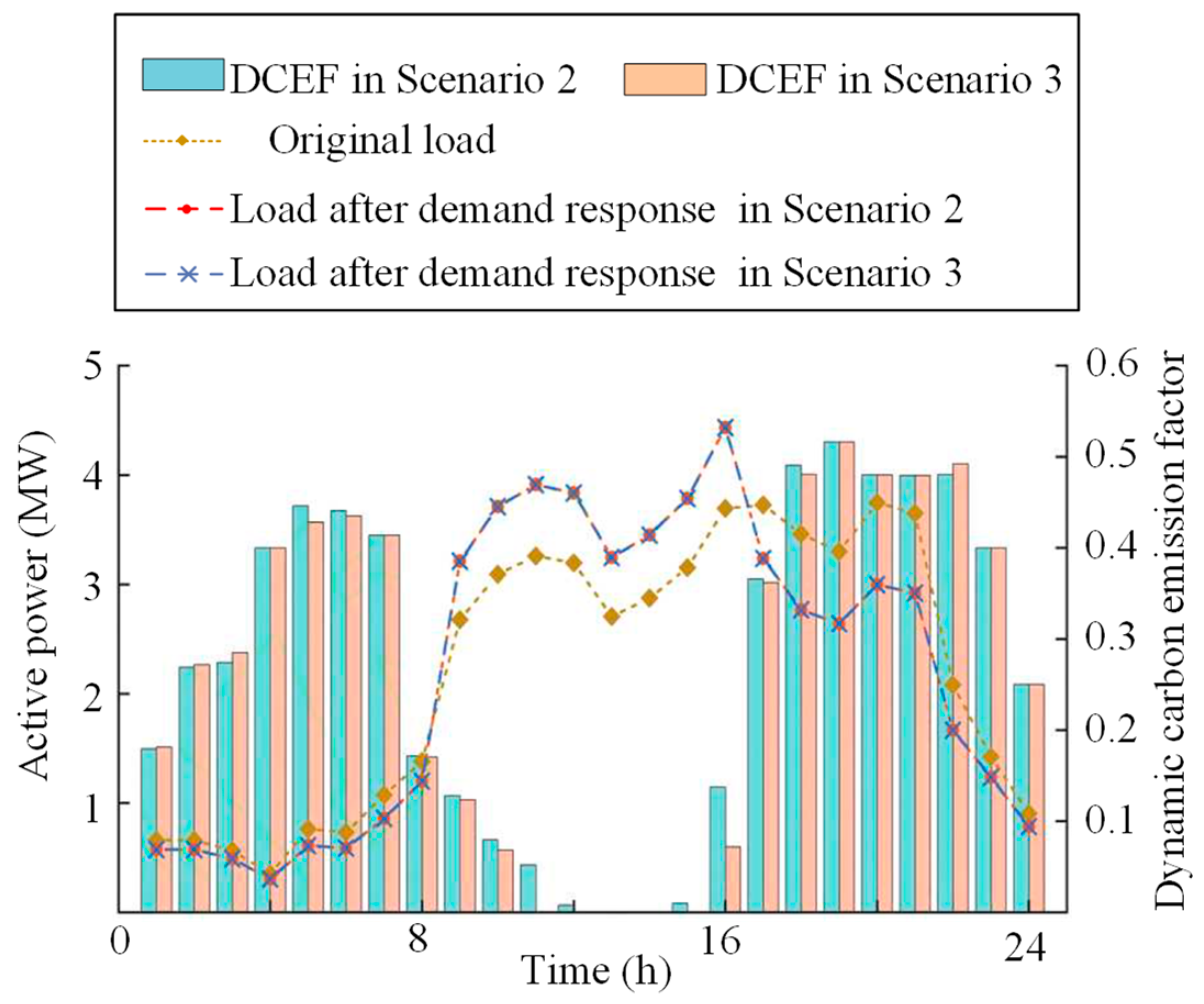
2.2. Dynamic Demand Response Model

The DCEF reflects the carbon emissions corresponding to the electricity consumption behavior of users at different moments in the scheduling cycle, and its mathematical model is

$$D_{{\mathrm{CO}}_2,t}=\left({\displaystyle \sum }_{j=1}^{N_n}{P}_{j,t}^{\mathrm{load}}{w}_{j,t}\right)/\left({\displaystyle \sum }_{j=1}^{N_n}{P}_{j,t}^{\mathrm{load}}\right)$$

(2)

where $N_n$ is the total number of nodes, $D_{{\mathrm{CO}}_2,t}$ is the DCEF of ADN at time $t$, and $P_{j,t}^{\mathrm{load}}$ is the active load of node $j$ at time $t$.

Price-based demand response is generally through the adjustment of the price of electricity to change the original electricity consumption plan. The degree of load response and the amount of price change is often expressed by the elasticity coefficient $\lambda$:

$$\lambda ={\displaystyle \frac{\mathsf{\Delta }P/P}{\mathsf{\Delta }C/C}}$$

(3)

where $P$ and $\mathsf{\Delta }P$ are electricity consumption and change in electricity consumption, and $C$ and $\mathsf{\Delta }C$ are electricity price and change in electricity price. The elasticity coefficient can be written in the following matrix form:

$$\mathit{H}=\left[\begin{array}{ccc}{\lambda }_{ll}& {\lambda }_{ln}& {\lambda }_{lh}\\ {\lambda }_{nl}& {\lambda }_{nn}& {\lambda }_{nh}\\ {\lambda }_{hl}& {\lambda }_{hn}& {\lambda }_{hh}\end{array}\right]$$

(4)

where ${\lambda }_{ll}, {\lambda }_{nn}$, and ${\lambda }_{hh}$ are the auto-elasticity coefficients for low-carbon, flat-carbon, and high-carbon time periods, respectively. ${\lambda }_{ln}, {\lambda }_{ll}, {\lambda }_{nl}, {\lambda }_{nh}, {\lambda }_{hl}$, and ${\lambda }_{nn}$ are the mutual elasticity coefficients, respectively.

The load demand after implementing demand response can be expressed as

$$\left.\begin{array}{c}\left[\begin{array}{c}{P}_{1,1}\\ ⋮\\ P_{1,t}\\ ⋮\\ P_{1,T}\end{array}\right]=\left[\begin{array}{c}{P}_{0,1}\\ ⋮\\ P_{0,t}\\ ⋮\\ P_{0,T}\end{array}\right]+\left[\begin{array}{ccccc}{P}_{0,1}& & & & \\ & \ddots & & & \\ & & P_{0,t}& & \\ & & & \ddots & \\ & & & & P_{0,T}\end{array}\right]\\ \mathit{E}\\ \\ \\ \mathsf{\Delta }{C}_1/C_{0,1}\\ ⋮\\ \mathsf{\Delta }{C}_t/C_{0,t}\\ ⋮\\ \mathsf{\Delta }{C}_T/C_{0,T}\end{array}\right]$$

(5)

where $P_{0,t}$ and $P_{1,t}$ are the load demand before and after the implementation of demand response at time $t$, and $\mathsf{\Delta }{C}_t/C_{0,t}$ is the rate of change of electricity price at time $t$. The $\mathit{E}$ matrix is extended from the elasticity matrix $\mathit{H}$, and $T$ is the scheduling period.

Taking one day as the scheduling cycle, according to the DCEF changes, the introduction of large and small fuzzy affiliation functions determines the high-carbon time period and low-carbon time period, and the rest of the time period is the flat-carbon time period; that is

$$\left\{\begin{array}{l}{u}_{\mathrm{A}}={\displaystyle \frac{D_{{\mathrm{CO}}_2,t}-D_{{\mathrm{CO}}_2,\min }}{D_{{\mathrm{CO}}_2,\max }-D_{{\mathrm{CO}}_2,\min }}}\hfill \\ u_{\mathrm{B}}={\displaystyle \frac{D_{{\mathrm{CO}}_2,\max }-D_{{\mathrm{CO}}_2,t}}{D_{{\mathrm{CO}}_2,\max }-D_{{\mathrm{CO}}_2,\min }}}\hfill \end{array}\right.$$

(6)

where $u_{\mathrm{A}}$ and $u_{\mathrm{B}}$ are the high-carbon affiliation and low-carbon affiliation, and $D_{{\mathrm{CO}}_2,\max }$ and $D_{{\mathrm{CO}}_2,\min }$ are the maximum DCEF and the minimum DCEF.

3. Double-Level Optimization Model

The ADN optimization model proposed in this paper is a two-level optimization operation model. The upper-level model is the optimal economic scheduling model. The upper-level model is solved to obtain the optimal scheduling of PV and storage, the switch action of each time period, and the distribution of the system power flow. Based on the results of the upper-level model, the carbon potential and DCEF of each node are calculated and substituted into the lower-level-demand response model. The load data is updated according to the lower-level-demand response results and substituted into the upper-level economic scheduling model.

3.1. Upper-Level Optimization Model

3.1.1. Objective Function

The upper-level model has its objective function to minimize the sum of network losses and solar curtailment penalty cost $F_1$, i.e.,

$$\min F_1={\displaystyle \sum }_{t=1}^T{\displaystyle \sum }_{ij\in {\xi }^{\mathrm{Line}}}{C}_{\mathrm{loss}}{I}_{ij,t}^2{R}_{ij}\mathsf{\Delta }t+{\displaystyle \sum }_{t=1}^T{\displaystyle \sum }_{i\in {\xi }^{\mathrm{PV}}}{C}_{\mathrm{pvloss}}\left(P_{i,t}^{\mathrm{PV},\mathrm{Pre}}-P_{i,t}^{\mathrm{PV}}\right)\mathsf{\Delta }t$$

(7)

where ${\xi }^{\mathrm{Line}}$ is the set of all branches; ${\xi }^{\mathrm{PV}}$ is the set of nodes accessing PV in the ADN; $C_{\mathrm{loss}}$ and $C_{\mathrm{pvloss}}$ are the network loss and solar curtailment cost; $P_{i,t}^{\mathrm{PV},\mathrm{Pre}}$ and $P_{i,t}^{\mathrm{PV}}$ are the predicted PV active power of node $i$ and the active power actually injected into node $i$ at time t; and $I_{ij,t}$ is the current RMS value of branch $ij$ at time $t$.

3.1.2. Constraints

(a)

DistFlow constraints

The DistFlow model takes the branch power as the object of study and is commonly used in AC distribution networks with the mathematical model [27]:

$${\displaystyle \sum }_{k\in \alpha \left(j\right)}{P}_{jk,t}-{\displaystyle \sum }_{i\in \beta \left(j\right)}\left(P_{ij,t}-I_{ij,t}^2{R}_{ij}\right)=P_{j,t}^{\mathrm{in}}$$

(8)

$${\displaystyle \sum }_{k\in \alpha \left(j\right)}{Q}_{jk,t}-{\displaystyle \sum }_{i\in \beta \left(j\right)}\left(Q_{ij,t}-I_{ij,t}^2{X}_{ij}\right)=Q_{j,t}^{\mathrm{in}}$$

(9)

$$U_{j,t}^2=U_{i,t}^2-2\left(R_{ij}{P}_{ij,t}+X_{ij}{Q}_{ij,t}\right)+\left(R_{ij}^2+X_{ij}^2\right)I_{ij,t}^2$$

(10)

$$I_{ij,t}^2{U}_{i,t}^2=P_{ij,t}^2+Q_{ij,t}^2$$

(11)

$$P_{j,t}^{in}=P_{j,t}^{sub}+P_{j,t}^{PV}+P_{j,t}^{ESS,dch}-P_{j,t}^{ESS,ch}-P_{j,t}^{load}$$

(12)

$$Q_{j,t}^{in}=Q_{j,t}^{sub}-Q_{j,t}^{ioad}$$

(13)

where $\alpha \left(j\right)$ is the set of downstream nodes with node $j$ as the upstream node of the branch; $\beta \left(j\right)$ is the set of upstream nodes with node $j$ as the downstream node of the branch; $P_{ij,t}$ and $Q_{ij,t}$ are the active and reactive power flowing through branch $ij$ at time t; $P_{jk,t}$ and $Q_{jk,t}$ are the active and reactive power flowing through the downstream branch with node $j$ as the upstream node at time t; $P_{j,t}^{\mathrm{in}}$ and $Q_{j,t}^{\mathrm{in}}$ are the active and reactive power injected into the node $j$ at time t; $P_{j,t}^{\mathrm{ESS},\mathrm{dch}}$ and $P_{j,t}^{\mathrm{ESS},\mathrm{ch}}$ are the charging and discharging power of the energy storage device of node j at time t; $P_{j,t}^{\mathrm{sub}}$ and $Q_{j,t}^{\mathrm{sub}}$ are the active and reactive power injected at node $j$ at time $t$; $Q_{j,t}^{\mathrm{Ioad}}$ is the reactive power load of node $j$ at time $t$; $U_{j,t}$ is the voltage RMS value of node $j$ at time $t$; and $R_{ij}$ and $X_{ij}$ are the equivalent resistance and reactance of branch $ij$.

Due to the presence of nonlinear terms in the above equations, which are generally difficult to solve directly. They are linearly transformed using intermediate variables as well as second order cone relaxation [28]. Let $I_{ij,t}^{\mathrm{sqrt}}=I_{ij,t}^2,U_{j,t}^{\mathrm{sqrt}}=U_{j,t}^2$ replace the squared term in (8)~(11), i.e.,

$${\displaystyle \sum }_{k\in \alpha \left(j\right)}{P}_{jk,t}-{\displaystyle \sum }_{i\in \beta \left(j\right)}\left(P_{ij,t}-I_{ij,t}^{\mathrm{sqrt}}{R}_{ij}\right)=P_{j,t}^{\mathrm{in}}$$

(14)

$${\displaystyle \sum }_{k\in \alpha \left(j\right)}{Q}_{jk,t}-{\displaystyle \sum }_{i\in \beta \left(j\right)}\left(Q_{ij,t}-I_{ij,t}^{\mathrm{sqrt}}{X}_{ij}\right)=Q_{j,t}^{\mathrm{in}}$$

(15)

$$U_{j,t}^{\mathrm{sqrt}}=U_{i,t}^{\mathrm{sqrtt}}-2\left(R_{ij}{P}_{ij,t}+X_{ij}{Q}_{ij,t}\right)+\left(R_{ij}^2+X_{ij}^2\right)I_{ij,t}^{\mathrm{sqrt}}$$

(16)

$$I_{ij,t}^{\mathrm{sqrt}}{U}_{i,t}^{\mathrm{sqrt}}=P_{ij,t}^2+Q_{ij,t}^2$$

(17)

There is a nonlinear term in (17), which is converted to a second-order cone constraint using the second-order cone relaxation method, i.e.,

$$I_{ij,t}^{\mathrm{sqrt}}{U}_{i,t}^{\mathrm{sqrt}}⩾P_{ij,t}^2+Q_{ij,t}^2\iff {‖\begin{array}{l}2P_{ij,t}\\ 2Q_{ij,t}\\ I_{ij,t}^{\mathrm{sqrt}}-U_{i,t}^{\mathrm{sqrt}}\end{array}‖}_2⩽I_{ij,t}^{\mathrm{sqrt}}+U_{i,t}^{\mathrm{sqrt}}$$

(18)

After performing ADN dynamic reconfiguration, not all the branches satisfy (16), as some of them are in disconnected states, so (16) is further converted using the large M method [7]:

$$U_{j,t}^{\mathrm{sqrt}}-U_{i,t}^{\mathrm{sqrt}}⩽M{a}_{ij,t}-2\left(R_{ij}{P}_{ij,t}+X_{ij}{Q}_{ij,t}\right)+\left(R_{ij}^2+X_{ij}^2\right)I_{ij,t}^{\mathrm{sqrt}}$$

(19)

$$U_{j,t}^{\mathrm{sqrt}}-U_{i,t}^{\mathrm{sqrt}}⩾-M{a}_{ij,t}-2\left(R_{ij}{P}_{ij,t}+X_{ij}{Q}_{ij,t}\right)+\left(R_{ij}^2+X_{ij}^2\right)I_{ij,t}^{\mathrm{sqrt}}$$

(20)

where $M$ is a large enough positive number and $a_{ij,t}$ is a Boolean variable indicating the connected and disconnected status of branch $ij$ at time $t$. When $a_{ij,t}=0$, branch $ij$ is connected, and when $a_{ij,t}=1$, branch $ij$ is disconnected.

(b)

Node voltage and branch current constraints

To satisfy ADN operational safety, the node voltages and branch currents must be limited within specified ranges, i.e.,

$$U_{j,\min }^2⩽U_{j,t}^{\mathrm{sqrt}}⩽U_{j,\max }^2$$

(21)

$$0⩽I_{ij,t}^{\mathrm{sqrt}}⩽I_{ij,\max }^2$$

(22)

where $U_{j,\max }$ and $U_{j,\min }$ are the maximum and minimum voltages of node $j$ and $I_{ij,\max }$ is the maximum current flow through branch $ij$.

(c)

PV Output Constraints

Considering the different characteristics of PV outputs, different upper limits are set to constrain the PV outputs, which are constrained as

$$0⩽P_{j,t}^{\mathrm{PV}}⩽P_{j,t}^{\mathrm{PV},\max }$$

(23)

where, $P_{j,t}^{\mathrm{PV},\max }$ is the maximum PV power of node $j$ at time $t$.

(d)

ESS operational constraints

To smooth the fluctuation of PV output and increase the PV consumption rate, ESS is usually configured in the ADN system, and the charging and discharging process of ESS needs to be limited in terms of charging and discharging states and power, with the following constraints:

$$0⩽{\epsilon }_{j,t}^{\mathrm{ESS},\mathrm{ch}}+{\epsilon }_{j,t}^{\mathrm{ESS},\mathrm{dch}}⩽1$$

(24)

$${\epsilon }_{j,t}^{\mathrm{ESS},\mathrm{ch}}{P}_{t,\min }^{\mathrm{ESS},\mathrm{ch}}⩽P_{j,t}^{\mathrm{ESS},\mathrm{ch}}⩽{\epsilon }_{j,t}^{\mathrm{ESS},\mathrm{ch}}{P}_{t,\max }^{\mathrm{ESS},\mathrm{ch}}$$

(25)

$${\epsilon }_{j,t}^{\mathrm{ESS},\mathrm{dch}}{P}_{t,\min }^{\mathrm{ESS},\mathrm{dch}}⩽P_{j,t}^{\mathrm{ESS},\mathrm{dch}}⩽{\epsilon }_{j,t}^{\mathrm{ESS},\mathrm{dch}}{P}_{t,\max }^{\mathrm{ESS},\mathrm{dch}}$$

(26)

$$E_{j,t+1}^{\mathrm{ESS}}=E_{j,t}^{\mathrm{ESS}}+{\eta }_{\mathrm{ch}}^{\mathrm{ESS}}{P}_{j,t}^{\mathrm{ESS},\mathrm{ch}}-{\eta }_{\mathrm{dch}}^{\mathrm{ESS}}{P}_{j,t}^{\mathrm{ESS},\mathrm{dch}}$$

(27)

$$E_{\min }^{\mathrm{ESS}}⩽E_{j,t+1}^{\mathrm{ESS}}⩽E_{\max }^{\mathrm{ESS}}$$

(28)

where ${\epsilon }_{j,t}^{\mathrm{ESS},\mathrm{ch}}$ and ${\epsilon }_{j,t}^{\mathrm{ESS},\mathrm{dch}}$ are the charging and discharging state of the ESS of node $j$ at time $t$, which are used to restrict the ESS to be only in the charging or discharging state; $P_{t,\max }^{\mathrm{ESS}}$ and $P_{t,\min }^{\mathrm{ESS},\mathrm{ch}}$ are the maximum and minimum charging power of the ESS at time $t$; $P_{t,\max }^{\mathrm{ESS},\mathrm{dch}}$ and $P_{t,\min }^{\mathrm{ESS},\mathrm{dch}}$ are the maximum and minimum discharging power of the ESS at time $t$; $E_{j,t}^{\mathrm{ESS}}$ is the capacity of the ESS of node $j$ at time $t$; $E_{\max }^{\mathrm{ESS}}$ and $E_{\min }^{\mathrm{ESS}}$ are the maximum and minimum ESS capacities; and ${\eta }_{\mathrm{ch}}^{\mathrm{ESS}}$ and ${\eta }_{\mathrm{dch}}^{\mathrm{ESS}}$ are the ESS charging and discharging efficiency coefficients.

(e)

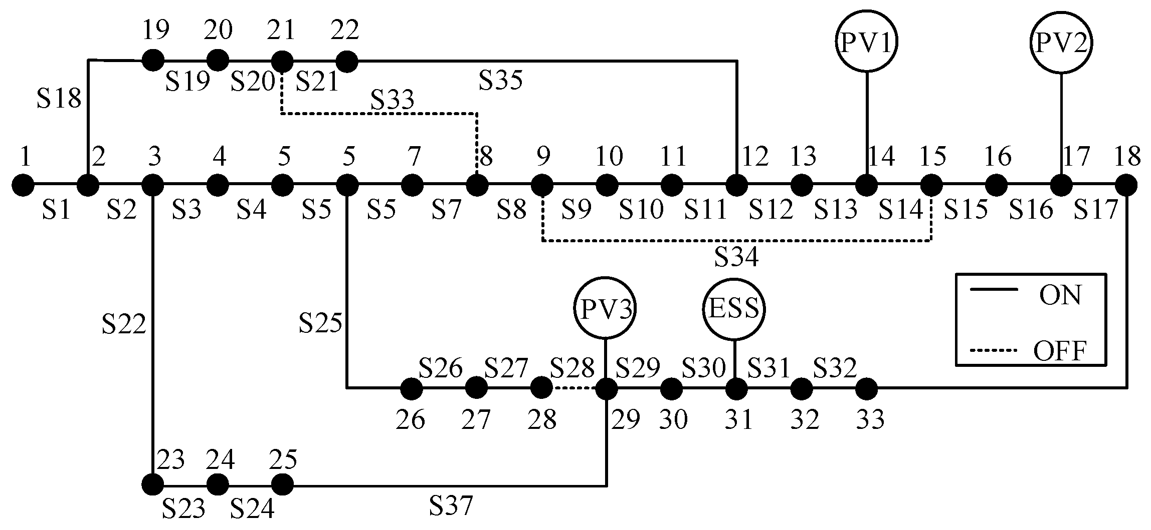
Topology constraints

In the upper-level optimization problem, it is necessary to ensure that the reconfigured ADN satisfies the radial structure; i.e., there are no islands and loops. In this paper, we adopt the radial topology constraint method [21], which is modeled as follows:

$${\displaystyle \sum }_{ij\in {\psi }_k}{a}_{ij}+{\displaystyle \sum }_{r\in {\psi }_k}{b}_r=1$$

(29)

$${\displaystyle \sum }_{r\in {\partial }_n}{b}_r⩽1$$

(30)

$${\displaystyle \sum }_{r\in {\partial }_n}{b}_r={\displaystyle \sum }_{ij\in {\partial }_n}{a}_{ij}$$

(31)

$${\displaystyle \sum }_{r\in {\phi }_m}{b}_r<N_{{\phi }_m}$$

(32)

where ${\psi }_k$ is the set of branches in the first $k$ basic loop; ${\partial }_n$ is the set of common branch loops in neighboring basic loops, i.e., ${\partial }_n={\psi }_{k1}\cap {\psi }_{k2}$; $b_r$ is the intermediate variable that replaces the common branch variable $a_{ij}$ in the neighboring basic loops so that the switches from each basic loop are independent of each other; $r$ is the branch corresponding to the converted intermediate variable $b_r$; ${\phi }_m$ and $N_{{\phi }_m}$ are the set of cutsets corresponding to node degree greater than or equal to three in the network and the number of branches in the corresponding cutsets.

3.2. Lower-Level Optimization Model

3.2.1. Objective Function

The lower-level model is based on the objective function of minimizing carbon emission on the load side as well as minimizing the cost of demand response scheduling.

Minimizing the total carbon emission

$$\min E_{{\mathrm{CO}}_2}=\min {\displaystyle \sum }_{t=1}^T{\displaystyle \sum }_{j=1}^{N_n}{P}_{j,t}^{\mathrm{load},\mathrm{DR}}{w}_{j,t}$$

(33)

where $P_{j,t}^{\mathrm{load},\mathrm{DR}}$ is the load level of node $j$ after demand response at time $t$.

Minimizing the demand response scheduling cost

$$\min C_{\mathrm{DR}}=\min {\displaystyle \sum }_{t=1}^T\left(P_{0,t}{C}_{0,t}-P_{1,t}{C}_{1,t}\right)$$

(34)

For the above multi-objective function, the weighting combination is used to transform it into a single-objective problem. Because of the different sizes of the two scales, the weighting needs to be normalized before processing, and ultimately results in the lower model objective function

$$\min F_2=\left(1-\alpha \right)E_{{\mathrm{CO}}_2}^{\prime }+\alpha C_{\mathrm{DR}}^{\prime }$$

(35)

where $\alpha$ is the weight factor.

3.2.2. Constraints

(a)

Total day-ahead load constraints

To satisfy the customer electricity demand, in the implementation of the demand response process it is required that the total amount of load remains unchanged during the scheduling cycle, i.e.,

$${\displaystyle \sum }_{t=1}^T{P}_{0,t}={\displaystyle \sum }_{t=1}^T{P}_{1,t}$$

(36)

(b)

Load-response constraints

The amount of load regulation during the scheduling cycle is subject to the following limitation:

$$\mathsf{\Delta }{P}_{t,\min }⩽P_{1,t}-P_{0,t}⩽\mathsf{\Delta }{P}_{t,\max }$$

(37)

where $\mathsf{\Delta }{P}_{t,\max }$ and $\mathsf{\Delta }{P}_{t,\min }$ are the upper and lower limits of adjustable load at time $t$.

(c)

Electricity price constraints

Electricity price should be set within limits:

$$C_{t,\min }⩽C_{1,t}⩽C_{t,\max }$$

(38)

where $C_{t,\max }$ and $C_{t,\min }$ are the upper and lower limits of the electricity price at time $t$.

(d)

User electricity cost constraints

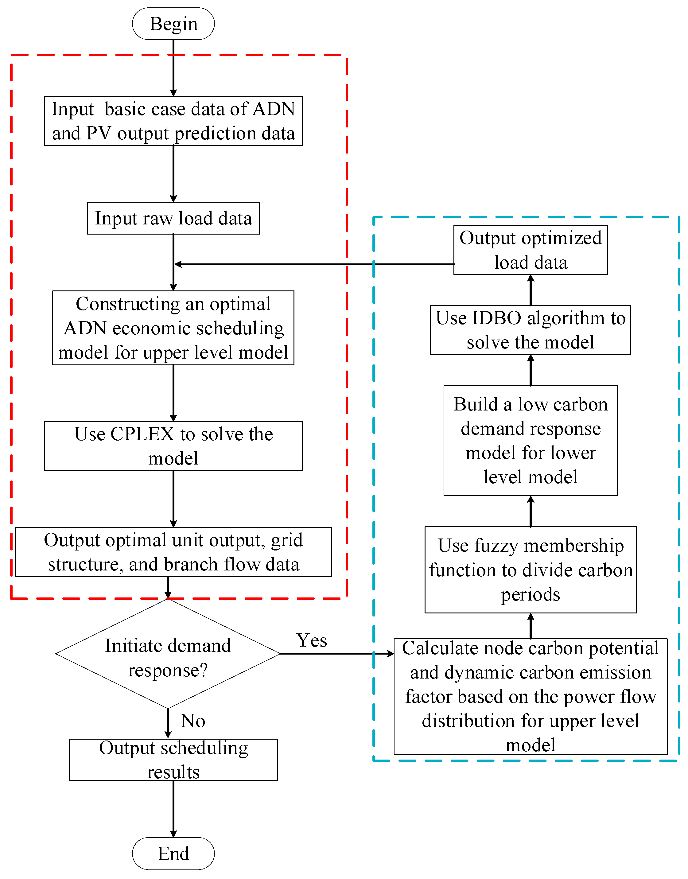
To ensure that customers are motivated to participate in demand response as well as benefit from it, it is required that the cost of electricity consumption after demand response is less than before demand response:

$${\displaystyle \sum }_{t=1}^T{P}_{0,t}{C}_{0,t}⩾{\displaystyle \sum }_{t=1}^T{P}_{1,t}{C}_{1,t}$$

(39)

4. Solution Method

4.1. Improved DBO Algorithmization

The dung beetle optimizer (DBO) algorithm is a new heuristic optimization algorithm based on the social behaviors of dung beetles, which not only has the characteristics of simple structure and strong optimization searching ability, but also suffers from local and global imbalance problems [24]. Therefore, to improve the search performance of the DBO algorithm, this paper adopts various strategies to improve it.

4.1.1. Chebyshev Maps the Initial Population

The random initialization of population method is used in the DBO algorithm, which leads to uneven distribution of dung beetles in the solution space and affects its convergence speed and accuracy. In this paper, Chebyshev chaotic mapping is added in the initialization of population in the DBO algorithm, which enhances the diversity of the initial population and makes its distribution more even in the whole solution space, as is shown below:

$$x_{n+1}=\cos \left(k\arccos x_n\right)$$

(40)

where $k$ is the order and $x_n$ is the position of the population individual at the iteration $n$, $x_n\in \left[-1,1\right]$.

4.1.2. Adaptive Weight and Variable Spiral Searching

To further improve the optimization performance of DBO, an adaptive variable spiral search strategy is introduced to improve the position of the dung beetle and adaptive inertia weights are added. The position of the improved theft phase is updated as

$${\eta }^{*}={\mathrm{e}}^{\gamma \cos \left(\pi t/S_{\max }^{\mathrm{Iter}})\right.}$$

(41)

$$\omega ={\omega }_{\min }+\left({\omega }_{\max }-{\omega }_{\min }\right)\arctan \left(\pi t/2S_{\max }^{\mathrm{Iter}}\right)$$

(42)

$$x_i^{t+1}=\omega x_{\mathrm{gbest}}^t+{\mathrm{e}}^{l{\eta }^{*}}\cos \left(2\pi l\right)\left(\left|x_i^t-x_{\mathrm{gbest}}^t\right|+\left|x_i^t-x_{\mathrm{lbest}}^t\right|\right)$$

(43)

where ${\eta }^{*}$ is the variable helix parameter; $\gamma$ is the adjustment factor; $S_{\max }^{\mathrm{Iter}}$ is the maximum number of iterations; $l$ is the random number $l\in \left[-1,1\right]$; $\omega$ is the weight coefficient; and $x_{\mathrm{gbest}}^t$ and $x_{\mathrm{lbest}}^t$ are the global and local optimal positions of the iteration $t$.

4.1.3. Optimal Positional Perturbation Strategy

The DBO algorithm gradually approaches the optimal individual in the later iterations, leading to a decrease in the diversity of the population. To reduce the possibility of its falling into local optimality, this paper perturbs the optimal dung beetle individuals through two perturbation strategies, namely, equal probability alternating selection of Cauchy mutation and refractive inverse learning, as is shown below:

$$x_{\mathrm{new},\mathrm{gbest}}^t=\left\{\begin{array}{l}{\displaystyle \frac{l_b+u_b}{2}}+{\displaystyle \frac{l_b+u_b}{2\delta }}-{\displaystyle \frac{x_{\mathrm{gbest}}^t}{\delta }},\mathrm{rand}()<0.5\\ x_{\mathrm{gbest}}^t+\mathrm{Cauchy}\left(0,1\right)x_{\mathrm{gbest}}^t,\mathrm{rand}()⩾0.5\end{array}\right.$$

(44)

where $x_{\mathrm{new},\mathrm{gbest}}^t$ is the new individual after perturbation; $l_b$ and $u_b$ are the upper and lower bounds of the variables; and $\delta$ is the refractive index of light, which varies with the number of iterations. Cauchy $\left(0,1\right)$ is the standard Cauchy distribution.

Since it is not possible to confirm that the mutated optimal fitness is better than the original fitness, this paper chooses whether to update the position or not by a greedy strategy.

4.2. Model Solving

The model solution flow is shown in Figure 2.

The upper ADN operation optimization model is converted into a mixed integer second-order cone planning model after linear transformation and second-order cone relaxation, which can be solved by CPLEX commercial solver, and there are both continuous and discrete variables in its decision variables. Theoretically, the switch state at each moment in the scheduling cycle should be defined as a variable. However, as the time period increases, the number of discrete variables and the search space of the solution also increase greatly, which greatly affects the solution efficiency, and the number of dynamic reconfigurations should be limited in order to ensure that the service life of the switch is within the normal range in practice. Therefore, this paper adopts the time period division method based on improved recursive ordered clustering to divide the discrete equipment regulation cycle, and the dynamic reconstruction only occurs at the initial moment of each time period.

The lower-level optimization model is solved using IDBO. Since the load levels change after the demand response, it is necessary to correct the load data in the upper-level model and re-solve the economic scheduling model.

5. Case Study

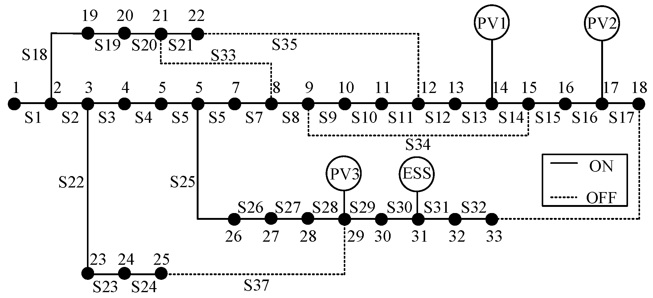
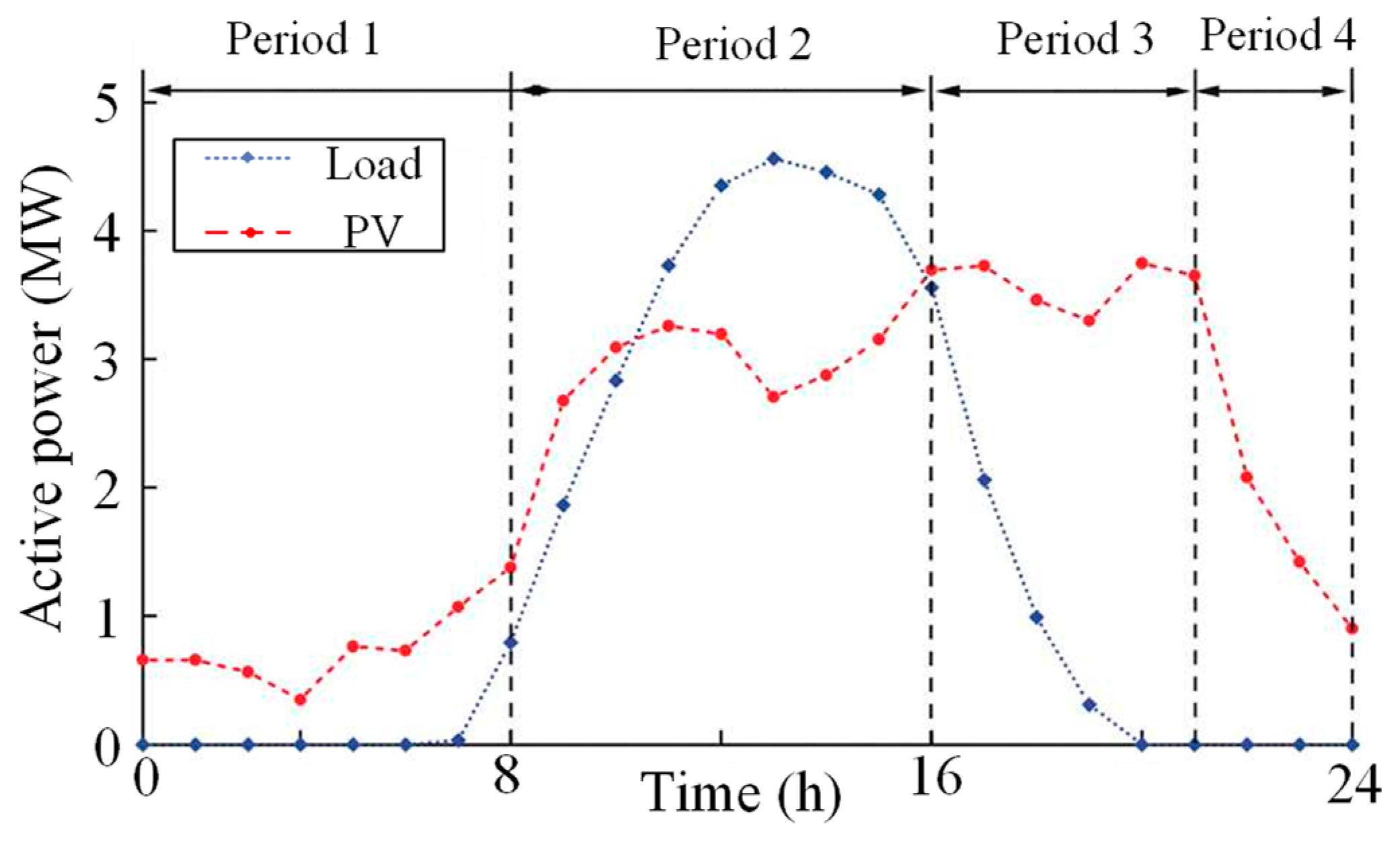
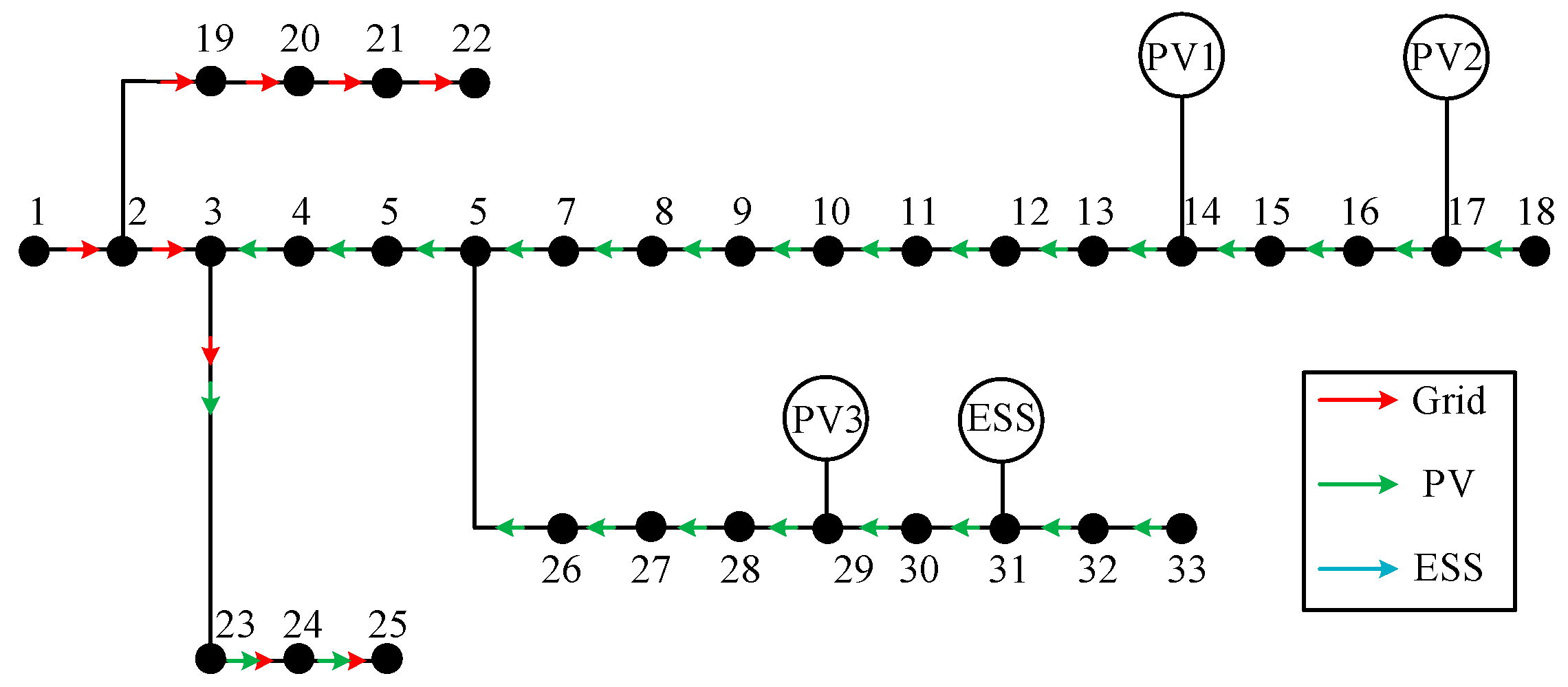
5.1. Simulation Setup

To verify the effectiveness of the method proposed in this paper, simulations are performed based on the improved IEEE 33 node system [29]. The network topology is shown in Figure 3. On this basis, PV arrays PV₁, PV₂, and PV₃ with rated capacities of 1500 kW are accessed for nodes 14, 17, and 29, respectively. The ESS with a rated capacity of 1000 kWh is accessed at node 31, which has a rated charging and discharging power of 150 kW and maximum charging and discharging efficiencies of 0.9. The day-ahead predicted load power of each node at each time slot is obtained based on the load ratio and load distribution in [30]. PV power curves are calculated with reference to [30] and shown in Figure 4, along with the reconfiguration time slot division results and load. The network loss and solar curtailment penalty referred to [31] and the tariff elasticity matrix data referred to [26]. The ideal operating voltage is set as [0.95, 1.05]. The scheduling period is 24 h with a step size of 1 h, and three different scenarios are set up: Scenario 1 is the traditional ADN optimization. Scenario 2 is ADN optimization using demand response. Scenario 3 is ADN optimization using dynamic reconfiguration with demand response.

5.2. Scheduling Results Analysis

5.2.1. Economics in Different Scenarios

Compared to Scenario 1 and Scenario 2, Scenario 3 uses a low-carbon-demand response, so the load curve will change compared to the original curve. The DCEF can be calculated from the upper optimization result. On this basis, the fuzzy genus function is used to adjust the small segments, and the 24 h in a cycle is divided into three electricity consumption periods of high carbon, flat carbon, and low carbon, with each period lasting 8 h. The specific time period division results are shown in

Table 2. Results of the division of high- and low-carbon time periods.

Time Slot Type	Time Division
High carbon	5:00–7:00, 18:00–22:00
Flat carbon	1:00–4:00, 7:00–8:00, 17:00–18:00, 23:00–24:00
Low carbon	9:00–16:00

, and the load curve and the DCEF are shown in Figure 5.

As can be seen in Figure 5, after considering the low-carbon-demand response, the load is shifted from the high-carbon period to the low-carbon period and the load is reduced during the flat carbon period, which not only reduces the peak-to-valley difference of the load and improves the balance of the ADN, but also increases the consumption of renewable energy sources because of the shifting of the variable load electricity consumption time and the use of low carbon energy sources as much as possible. The direction of ADN carbon flow for Scenario 2 is shown in Figure 6, the system topology after dynamic reconfiguration for Scenario 3 is shown in Figure 7, and the comparison of economic performance in different scenarios is shown in

Table 3. Scheduling results for the three different scenarios.

Scenario	Time	OFF Branch	O&M Cost ($)	Network Loss Cost ($)	Solar Curtailment Cost ($)	Scheduling Cost ($)	Carbon Emission (kg)
1	All hours	S33, S34, S35, S36, S37	1696.82	595.04	1101.78	0	13,408.56
2	All hours	S33, S34, S35, S36, S37	1562.46	587.76	718.26	256.44	12,704.71
3	1:00–8:00	S7, S9, S16, S28, S34	1054.89	304.53	493.92	256.44	11,500.96
	9:00–16:00	S7, S9, S16, S26, S33
	17:00–21:00	S7, S9, S16, S28, S34
	22:00–24:00	S7, S9, S14, S32, S37

. O&M cost equals the sum of network loss cost, solar curvature cost, and scheduling cost.

As can be seen from Table 3, Scenario 1 adopts the traditional scheduling strategy and does not consider the impact of carbon emissions, which results in high network losses, solar curtailment cost, and system carbon emissions. Compared with Scenario 1, the use of the low-carbon demand response in Scenario 2 results in a reduction of 34.81% in the solar curtailment cost from USD 101.78 to USD 718.26, a decrease of 34.81%, a slight reduction in network loss, and a reduction of 7.92% in the total system operating cost from USD 1696.82 to USD 1562.46, and a reduction of 5.24% in carbon emissions from 13,408.56 kg to 12,704.71 kg. Comparing Scenario 2 and Scenario 3, it can be seen that considering dynamic reconfiguration, the network loss as well as the cost of discarding PV is reduced by 48.19% and 31.23%, while the carbon emissions of the system are reduced by 9.47% by cooperating with the mutual action of some switches. The above results show that the joint optimization proposed in this paper effectively improves ADN operation and has a good effect on improving the economy of ADN as well as promoting renewable energy consumption.

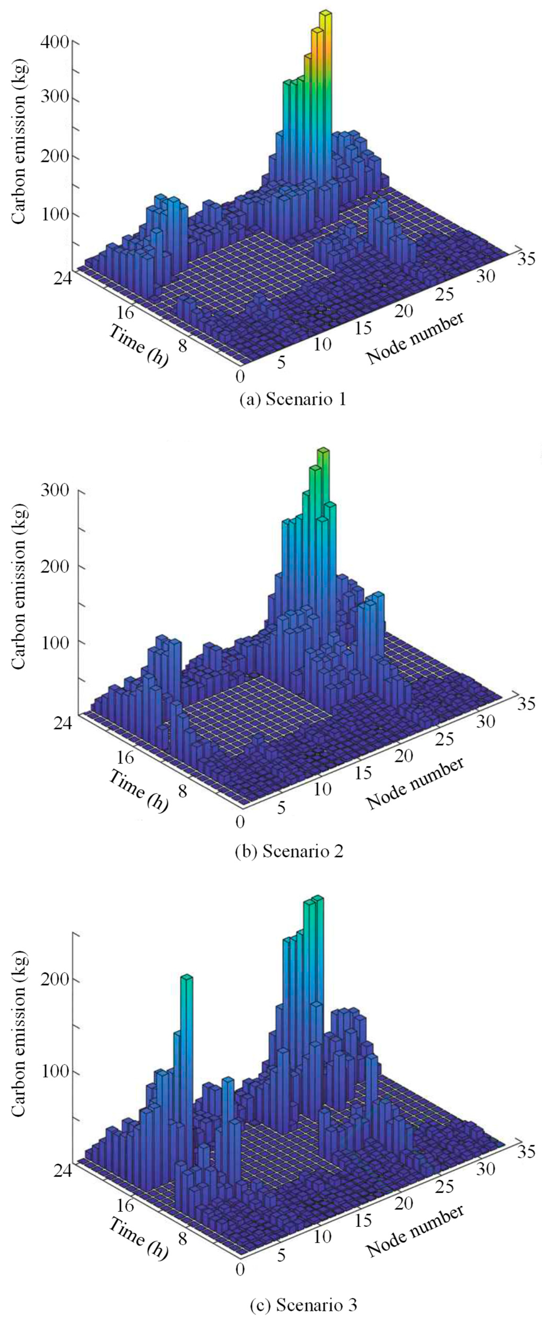
5.2.2. Carbon Emissions in Different Scenarios

The node carbon emissions for the three different scenarios are shown in Figure 8.

As can be seen from Figure 8, the main difference between Scenario 2, Scenario 3, and Scenario 1 is that the nodal carbon emissions reduce in the periods from 5:00 to 7:00 and from 18:00 to 22:00, because the implementation of price-based demand response guided by the DCEF changes user’s electricity consumption habits on the time scale, and some of the loads in the high-carbon time period with a large DCEF are shifted to the low-carbon time period with a small DCEF. However, in some moments the total load is larger than the PV output and the carbon emissions in some nodes increase in order to prevent voltage overruns. The shift of some loads from the high-carbon period with a large dynamic carbon factor to the low-carbon period with a small dynamic carbon factor, however, resulted in higher carbon emissions at some nodes in some moments when the total load after the shift was larger than the PV output and in order to prevent voltage overruns. Nevertheless, the overall carbon emissions were still reduced in the overall view. Comparing Scenario 2 with Scenario 3, the main difference was that in Scenario 3, during the period from 9:00 to 16:00, the carbon emissions of node 3~7 increased, but the carbon emissions of node 20~25 greatly reduced, because Scenario 3 considered dynamic reconfiguration to change the topology of the network, which consumed the PV output power cut due to voltage overrun, reduced the node carbon emissions, and at the same time changed the range of the PV energy supply.

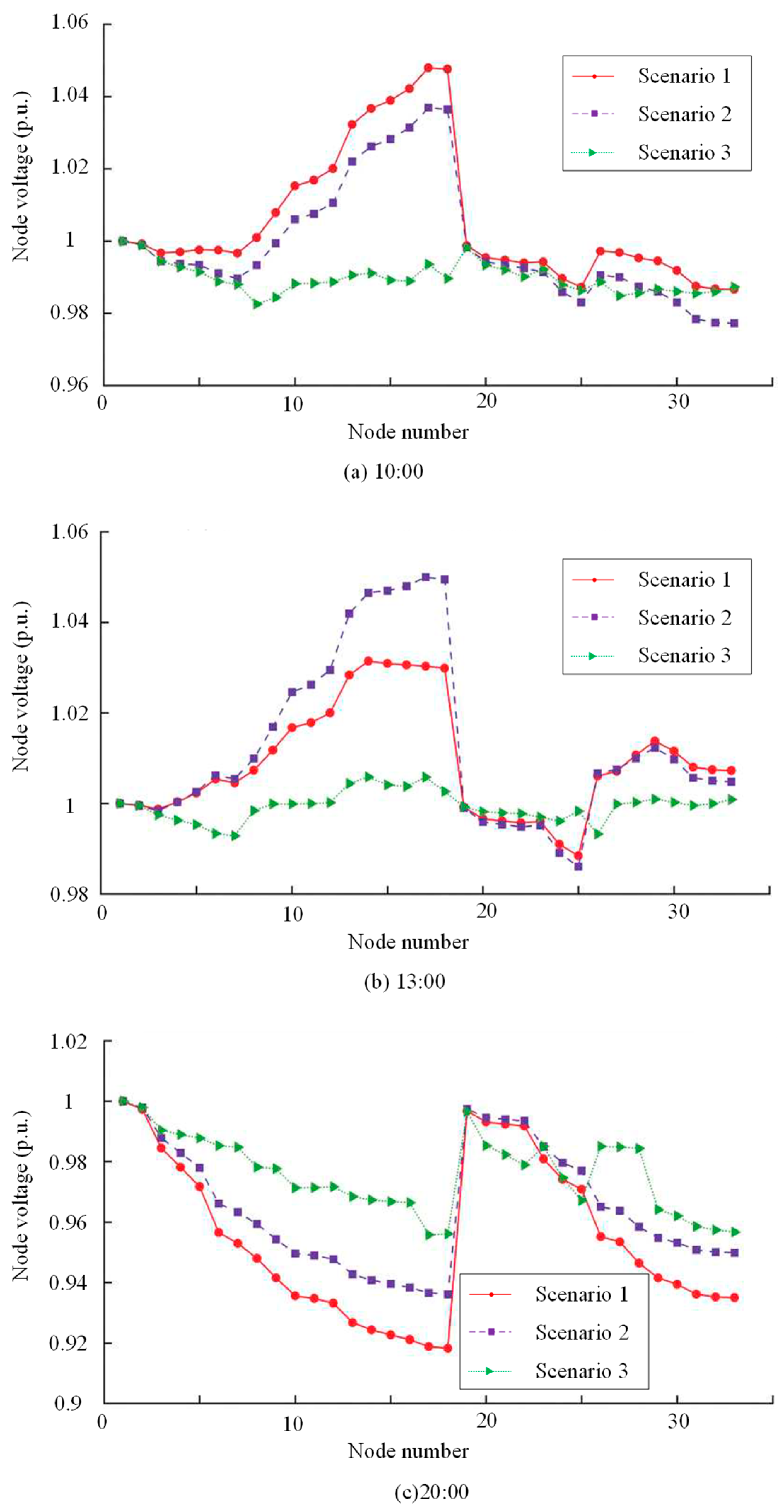
5.2.3. Node Voltage in Different Scenarios

The results of the effect of different scheduling strategies on the system voltage are shown in

Table 4. System voltage offsets for different scenarios.

Scenario	Total Voltage Offset
1	0.4006
2	0.3518
3	0.2281

, and the results are used as standardized values.

To further verify the enhancement of the proposed method on the system voltage control level, three typical moments are selected, which are the moment when the PV output prediction value is similar to the load level ($10:00$), the moment when the PV output prediction value is larger and the load level is lower ($13:00$), and the moment when the PV has no output and the load level is larger ($20:00$). The voltage distributions at different moments are shown in Figure 9.

Figure 9a shows that when the PV output is similar to the load level, the highest voltage in Scenario 1 occurs at node 17, reaching 1.048. This value approaches the upper operational limit, posing a risk of overvoltage. After incorporating a low-carbon demand response in Scenario 2, the maximum voltage drops to 1.036. This reduction occurs because the total load level increases under a low-carbon demand response, while the PV output has already reached its maximum before demand response activation. Figure 9b reveals that during periods of high PV output and relatively low load, the maximum voltage in Scenario 1 is 1.030. However, in Scenario 2 with low-carbon-demand response, the load level increases and the PV output increases correspondingly, causing the system voltage to rise to 1.050. This reaches the upper operational limit, creating an overvoltage risk, necessitating PV output curtailment. Figure 9c demonstrates that when there is no PV output and the load level is high, the minimum voltage in Scenario 1 drops to 0.918, significantly deviating below the lower operational limit. Implementing a low-carbon-demand response raises the minimum voltage to 0.937. This improvement arises because the demand response reduces the total system load, thereby increasing the overall voltage profile, although it remains below the ideal operating voltage.

Critically, under all conditions, Scenario 3, which further incorporates dynamic reconfiguration, achieves a substantial improvement in node voltage quality. This effectively mitigates the risk of power accidents caused by voltage limit violations and ensures that the secure operation requirements of the distribution network are met.

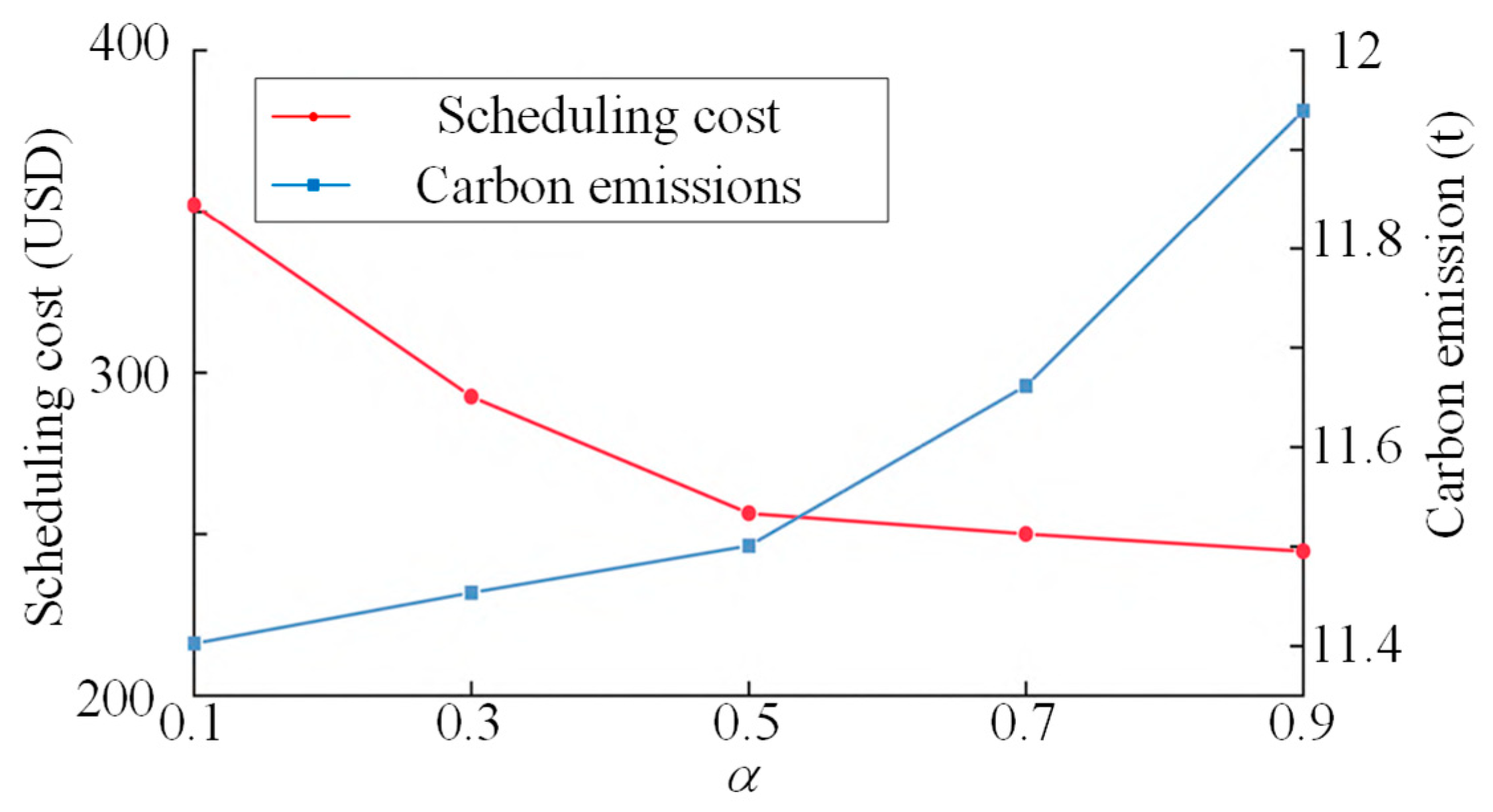
5.2.4. Optimization Results with Different Weights

The impact of different weights in the lower tier demand response on the optimization results is shown in Figure 10, which shows that as the weight $\alpha$ rises, the overall trend in the scheduling cost required to implement demand response decreases, and the trend in the decrease in scheduling cost is more moderate when $\alpha \in \left[0.5,1\right]$ is used. On the contrary, the total system carbon emissions gradually increase. Due to the conflict between the two, in order to take into account the scheduling cost and the total carbon emissions of the system, the fuzzy decision-making method is used to select a compromise solution [26], and the final value of $\alpha$ is taken as 0.5.

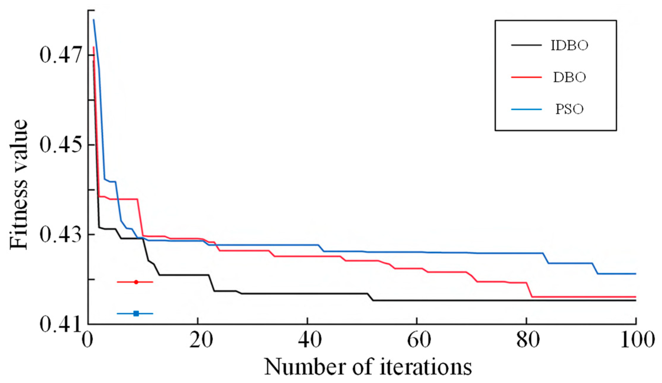
5.3. Performance Analysis of IDBO Algorithm

In order to verify the performance of the IDBO algorithm proposed in this paper, the particle swarm optimization (PSO) algorithm [19], DBO algorithm, and IDBO algorithm are used to jointly solve the ADN optimization scheduling problem in Scenario 3. For example, the population size is set to be 30 and the number of iterations is 100, in which the PSO learning factors c₁ and c₂ are both 1.5, the DBO parameters refer to [24], the proportion of rolling, breeding, fed, and stealing dung beetles in IDBO are 20%, 20%, 25%, and 35%, respectively, k is 0.1, b is 0.3, ${\omega }_{\max }$ is 0.89, and ${\omega }_{\min }$ is 0.1. The iteration curves are shown in Figure 11 and the fitness is weighted by normalization.

As can be seen from Figure 11, the PSO algorithm has weak convergence as well as a weak global search capability for the same number of populations and iterations. In contrast, IDBO improves DBO by incorporating multiple strategies to enhance its convergence performance; IDBO converges to the minimum objective function after 49 iterations, while DBO converges to the minimum objective function after 81 iterations. In terms of global search capability, DBO and IDBO perform similarly. In summary, IDBO has better convergence as well as global search ability. The comparison of calculation time for different methods is shown in Table 4. IDBO has the fastest computing speed, about 1.5 times that of DBO and 2 times that of PSO.

Table 5. Solution time for different methods.

Method	Solution Time (s)
IDBO	13.22
DBO	20.52
PSO	26.13

shows that the method proposed in this paper has good computational performance and has the potential to be extended to large-scale systems.

6. Conclusions

This paper proposes a novel optimization strategy for the operation of distribution networks in terms of economy, security, and low carbon. The following conclusions are obtained through case studies:

• The method in this paper changes the network topology through reasonable regulation of ESS, PV, and dynamic reconfiguration, which can equalize the distribution of the current, effectively reducing the network loss, solar curtailment cost, and system operating cost, and at the same time solving the ADN voltage overrun problem.
• The simulation results based on the 33 node testing system show that, based on the theory of carbon emission flow, under the premise of not changing the total load demand and using the DCEF as a guiding signal, the system load is reasonably adjusted on the time scale, which can promote coordinated interaction between the supply side and the demand side, promote the consumption of new energy, reduce the operating costs of the power system, and significantly reduce the total carbon emissions of the system.
• The proposed IDBO optimization algorithm possesses good convergence and global search capability, which can effectively solve the demand response model in this paper.

References

1. Liu, K.; Ye, X.; Kang, T.; Li, Z.; Jia, D. A Fast Dynamic Simulation Method of an Active Distribution Network with Distributed Generations Based on Decomposition and Coordination. Energies 2024, 17, 287. [Google Scholar] [CrossRef]
2. Liu, K.; Li, Z.; Cui, Z.; Jia, D.; Ye, X.; Su, J. A Finite State Machine Model for Business Flow in Active Distribution Networks Considering the Multi-Flow Fusion Process. J. Sci. Ind. Res. 2024, 83, 517. [Google Scholar]
3. Man, Y.; Liu, M.; Wang, K. A Review and Prospect of Research on Situational Awareness Technology in Active Distribution Network. Electron. Sci. Technol. 2024, 37, 6. [Google Scholar]
4. Spampinato, C.; La Magna, P.; Valastro, S.; Smecca, E.; Arena, V.; Bongiorno, C.; Mannino, G.; Fazio, E.; Corsaro, C.; Neri, F. Infiltration of CsPbI3: EuI2 Perovskites into TiO2 Spongy Layers Deposited by Gig-Lox Sputtering Processes. Proc. Sol. 2023, 3, 347–361. [Google Scholar] [CrossRef]
5. Ungerland, J.; Poshiya, N.; Biener, W.; Lens, H. A Voltage Sensitivity Based Equivalent for Active Distribution Networks Containing Grid Forming Converters. IEEE Trans. Smart Grid 2023, 14, 2825. [Google Scholar] [CrossRef]
6. Liu, X.; Lin, X.; Qiu, H.; Li, Y.; Huang, T. Optimal Aggregation And Disaggregation for Coordinated Operation of Virtual Power Plant with Distribution Network Operator. Appl. Energy 2024, 376, 124142. [Google Scholar] [CrossRef]
7. Sun, X.; Sheng, Y.; Wu, C.; Cai, Q.; Lai, X. Comprehensive Evaluation of Interval Equalization of Power Quality in Active Distribution Network Based on CVAE-TS. J. Electr. Eng. Technol. 2023, 19, 83. [Google Scholar] [CrossRef]
8. Xu, L.; Fan, S.; Zhang, H.; Xiong, J.; Liu, C.; Mo, S. Enhancing Resilience and Reliability of Active Distribution Networks through Accurate Fault Location and Novel Pilot Protection Method. Energies 2023, 16, 7547. [Google Scholar] [CrossRef]
9. Li, X.; Han, X.; Yang, M. Risk-Based Reserve Scheduling for Active Distribution Networks Based on an Improved Proximal Policy Optimization Algorithm. IEEE Access 2023, 11, 15211. [Google Scholar] [CrossRef]
10. El-Sayed, W.T.; Awad, A.S.A.; Azzouz, M.A.; Shaaban, M.F. A New Economic Dispatch for Coupled Transmission and Active Distribution Networks via Hierarchical Communication Structure. IEEE Syst. J. 2023, 17, 6226. [Google Scholar] [CrossRef]
11. Athanasiadis, C.L.; Papadopoulos, T.A.; Kryonidis, G.C.; Pippi, K.D. A Benchmarking Testbed for Low-Voltage Active Distribution Network Studies. IEEE Open Access J. Power Energy 2023, 10, 104. [Google Scholar] [CrossRef]
12. Dutta, A.; Ganguly, S.; Kumar, C. MPC-Based Coordinated Voltage Control in Active Distribution Networks Incorporating CVR and DR. IEEE Trans. Ind. Appl. 2022, 58, 4309. [Google Scholar] [CrossRef]
13. Wang, R.; Wen, X.; Wang, X.; Fu, Y.; Zhang, Y. Low Carbon Optimal Operation of Integrated Energy System Based on Carbon Capture Technology, LCA Carbon Emissions and Ladder-Type Carbon Trading. Appl. Energy 2022, 311, 118664. [Google Scholar] [CrossRef]
14. Zhou, Y. Worldwide Carbon Neutrality Transition? Energy Efficiency, Renewable, Carbon Trading and Advanced Energy Policies. Energy Rev. 2023, 2, 100026. [Google Scholar] [CrossRef]
15. Yang, X.; Meng, L.; Gao, X.; Ma, W.; Fan, L.; Yang, Y. Low-Carbon Economic Scheduling Strategy for Active Distribution Network Considering Carbon Emissions Trading and Source-Load Side Uncertainty. Electr. Power Syst. Res. 2023, 223, 109672. [Google Scholar] [CrossRef]
16. Mostafaeipour, A.; Bidokhti, A.; Fakhrzad, M.-B.; Sadegheih, A.; Mehrjerdi, Y.Z. A New Model for the Use of Renewable Electricity to Reduce Carbon Dioxide Emissions. Energy 2022, 238, 121602. [Google Scholar] [CrossRef]
17. Jiang, C.; Lin, Z.; Liu, C.; Chen, F.; Shao, Z. Shao MADDPG-Based Active Distribution Network Dynamic Reconfiguration with Renewable Energy. Prot. Control. Mod. Power Syst. 2024, 9, 143. [Google Scholar] [CrossRef]
18. Azizi, A.; Vahidi, B.; Nematollahi, A.F. Nematollahi Reconfiguration of Active Distribution Networks Equipped with Soft Open Points Considering Protection Constraints. J. Mod. Power Syst. Clean Energy 2023, 11, 212. [Google Scholar] [CrossRef]
19. Yan, R.; Yuan, Y.; Wang, Z.; Geng, G.; Jiang, Q. Active Distribution System Synthesis via Unbalanced Graph Generative Adversarial Network. IEEE Trans. Power Syst. 2023, 38, 4293. [Google Scholar] [CrossRef]
20. Mehrbakhsh, A.; Javadi, S.; Aliabadi, M.H.; Radmanesh, H. A Robust Optimization Framework for Scheduling of Active Distribution Networks Considering DER Units and Demand Response Program. Sustain. Energy Grids Netw. 2022, 31, 100708. [Google Scholar] [CrossRef]
21. Mahmoodi, S.; Tarimoradi, H. A Novel Partitioning Approach in Active Distribution Networks for Voltage Sag Mitigation. IEEE Access 2024, 12, 149206. [Google Scholar] [CrossRef]
22. Gorbachev, S.; Mani, A.; Li, L.; Zhang, Y. Zhang Distributed Energy Resources Based Two-Layer Delay-Independent Voltage Coordinated Control in Active Distribution Network. IEEE Trans. Ind. Inform. 2024, 20, 1220. [Google Scholar] [CrossRef]
23. Zhang, Z.; Dou, C.; Yue, D.; Zhang, Y.; Zhang, B.; Li, B. Regional Coordinated Voltage Regulation in Active Distribution Networks With PV-BESS. IEEE Trans. Circuits Syst. II Express Briefs 2023, 70, 596. [Google Scholar] [CrossRef]
24. Xue, J.; Shen, B. Dung Beetle Optimizer: A New Meta-Heuristic Algorithm for Global Optimization. J. Supercomput. 2023, 79, 7305. [Google Scholar] [CrossRef]
25. Huo, T.; Xu, L.; Feng, W.; Cai, W.; Liu, B. Dynamic Scenario Simulations of Carbon Emission Peak in China’s City-Scale Urban Residential Building Sector through 2050. Energy Policy 2021, 159, 112612. [Google Scholar] [CrossRef]
26. Egidy, S. Proportionality and Procedure of Monetary Policy-Making. Int. J. Const. Law 2021, 19, 285–308. [Google Scholar] [CrossRef]
27. Rigo-Mariani, R.; Vai, V. An Iterative Linear Distflow for Dynamic Optimization in Distributed Generation Planning Studies. Int. J. Electr. Power Energy Syst. 2022, 138, 107936. [Google Scholar] [CrossRef]
28. Cao, X.; Wang, J.; Zeng, B. A Study on the Strong Duality of Second-Order Conic Relaxation of AC Optimal Power Flow in Radial Networks. IEEE Trans. Power Syst. 2021, 37, 443–455. [Google Scholar] [CrossRef]
29. Abid, M.S.; Apon, H.J.; Morshed, K.A.; Ahmed, A. Optimal Planning of Multiple Renewable Energy-Integrated Distribution System with Uncertainties Using Artificial Hummingbird Algorithm. IEEE Access 2022, 10, 40716–40730. [Google Scholar] [CrossRef]
30. Sahu, S.K.; Kumari, S.; Ghosh, D.; Dutta, S. Dutta Estimation of Photovoltaic Hosting Capacity Due to the Presence of Diverse Harmonics in an Active Distribution Network. IEEE Access 2024, 12, 47868–47879. [Google Scholar] [CrossRef]
31. Klaes, M.; Zwartscholten, J.; Narayan, A.; Lehnhoff, S.; Rehtanz, C. Impact of ICT Latency, Data Loss and Data Corruption on Active Distribution Network Control. IEEE Access 2023, 11, 14693–14701. [Google Scholar] [CrossRef]
Figure 1. Schematic diagram of the carbon flow of an ADN.
Processes 13 01850 g001
Figure 2. Flowchart of the two-level model solution.
Processes 13 01850 g002
Figure 3. Improved IEEE 33 node system.
Processes 13 01850 g003
Figure 4. Graph of PV output and raw load profile.
Processes 13 01850 g004
Figure 5. DCEFs and load profiles before and after demand response.
Processes 13 01850 g005
Figure 6. Direction of ADN carbon flow at 10:00 in Scenario 2.
Processes 13 01850 g006
Figure 7. System topology after dynamic reconfiguration for Scenario 3.
Processes 13 01850 g007
Figure 8. Carbon emissions in different scenarios.
Processes 13 01850 g008
Figure 9. Voltage profiles at three typical moments. (a) Voltage amplitude at 10: 00; (b) Voltage amplitude at 13: 00; (c) Voltage amplitude at 20: 00.
Processes 13 01850 g009
Figure 10. Scheduling costs and total system carbon emissions at different weights.
Processes 13 01850 g010
Figure 11. Convergence curves of different algorithms.
Processes 13 01850 g011