Adsorption Column Performance Analysis for Volatile Organic Compound (VOC) Emissions Abatement in the Pharma Industry

Abstract

Volatile Organic Compounds (VOCs) are essential for primary pharmaceutical manufacturing. Their permissible emission levels are strictly regulated due to their toxic effects both on human health and the environment. Activated carbon adsorption columns are used in industry to treat VOC gaseous waste streams from industrial plants, but their process efficiency suffers from quick and unpredictable saturation of the adsorbent material. This study presents the application of a validated, non-isothermal, multicomponent adsorption model using the Langmuir Isotherm and the Linear Driving Force model to examine multicomponent VOC mixture breakthrough. Specifically, three binary mixtures (hexane–acetone, hexane–dichloromethane, hexane–toluene) are simulated for four different bed lengths (0.25, 0.50, 0.75, 1 m) and six different superficial velocities (0.1, 0.2, 0.3, 0.5, 0.7, 0.9 m s⁻¹). Key breakthrough metrics reveal preferential adsorption of acetone and toluene over hexane, and hexane over dichloromethane, as well as breakthrough onset patterns. Temperature peaks are moderate while pressure drops increase for longer column lengths and higher flow rates. A new breakthrough onset metric is introduced, paving the way to improved operating regimes for more efficient industrial VOC capture bed utilisation via altering multicomponent mixture composition, feed flowrate, and column length.

1. Introduction

Volatile organic compounds (VOC) are essential in life-saving medicine synthesis. As the pharmaceutical market experiences remarkable growth worldwide [1], the need for sustainable production increases alongside the demand for larger medicine volumes and the enforcing of stringent environmental regulations. Organic solvents are ubiquitous in reactions and separations for the production of active pharmaceutical ingredients, accounting for 56% of the overall mass balances [2,3]. The production of 1 kg of API requires on average the contribution of 46 kg of materials [3,4]. Since approximately 56% of the total process material required to produce APIs are solvents, almost 26 kg of solvents are required for the production of 1 kg of API. However, their emissions contribute to tropospheric ozone formation [5] and have adverse effects on human health [6]. Figure 1 illustrates the contribution of the pharmaceutical industry to VOC emissions in comparison with the overall VOC emissions by the industrial sector in China between 2013 and 2019 [7]; thus, for over a decade, a significant 6–9% originates from pharma manufacturing.

The design of more sustainable production processes and/or the use of “greener” solvents, although desirable, is more easily targeted than achieved. Henderson et al. stress that there is no silver bullet for solvent substitution [3]; although efforts such as solvent selection guides are widely used in the R&D phase for new products, the situation for established products is very complicated due to increased regulatory approval risks. Thus, end-of-pipe measures can ensure safe gas waste treatment.

In the field of industrial VOC emissions control, adsorption by activated carbon is the dominant method. This technology improves plant capability to filter gaseous trace pollutants from large-volume waste streams, with low operating costs and easy maintenance. Activated carbon is selected as adsorption material for VOCs [8] due to its unique hydrophobic and organophilic properties [9]. The VOC-laden air flow from preceding process unit vents is variable in concentration and mixture components, but also intermittent due to the several batch operation recipes carried out by these upstream units. Due to competitive adsorption between VOCs in a bed feed [10], a component’s bed outlet concentration may prematurely exceed the legal VOC emissions limit and thus require this industrial bed to be taken off-line for the adsorbent to be replaced. Thus, competitive adsorption results in the quick and unpredictable saturation of the adsorbent material which retains VOCs, thus requiring more frequent, expensive adsorbent changeovers.

Although adsorption beds are often operated in a cyclic manner (Temperature Swing Adsorption/TSA, Pressure Swing Adsorption/PSA, or more complex patterns), to ensure adsorbent regeneration and reuse, in many industrial settings where they constitute a counter-pollution measure instead of a production unit, adsorbent regeneration is outsourced, and thus beds are operated in a linear manner, until VOC emissions limits are reached on the column exit. In those situations, adsorbent saturation and time on stream until breakthrough onset drive operational decisions. Maximising time on stream before a changeover is necessary not only to ensure higher adsorbent utilisation, but also lower operating costs and overall carbon footprint due to outsourced material changeovers.

Over the years, adsorption has been widely studied, both on an experimental and computational level. Research on several parameters affecting adsorption bed operation, e.g., humidity [11,12,13,14], different adsorbents [15,16,17,18], and cyclic operation regimes [19,20,21], has enriched our understanding of the adsorption process [22,23] and helped address many operational pitfalls. Nevertheless, only a few experimental and modeling studies so far have explored adsorption in larger, industrial-length equipment, especially for varying feed flowrates and multicomponent VOC mixtures under realistic conditions [24,25,26].

This paper demonstrates the application of a validated, dynamic, non-isothermal, multicomponent adsorption model to investigate the effects of superficial velocity and column length on volatile organic compound (VOC) mixture adsorption. Specifically, the adsorption of three binary mixtures (with air as the carrier gas) is studied on four activated carbon fixed-bed columns, ranging from laboratory- to industrial-scale lengths (L = 0.25, 0.50, 0.75, 1 m), under six superficial velocities (V_s = 0.1, 0.2, 0.3, 0.5, 0.7, 0.9 m s⁻¹). Firstly, the simulation results regarding the breakthrough characteristics, temperature, and pressure drop trends of the mixtures of hexane–acetone, hexane–dichloromethane, and hexane–toluene are presented and analyzed for three superficial velocities (V_s = 0.1, 0.5, 0.9 m s⁻¹) and two bed lengths (L = 0.25, 1 m). Moreover, a new metric for bed design is introduced, based on the effect of the operating superficial velocity (V_s = 0.1, 0.2, 0.3, 0.5, 0.7, 0.9 m s⁻¹) on breakthrough onset times for different bed lengths (L = 0.25, 0.50, 0.75, 1 m), toward effective adsorption bed usage for multicomponent VOC mixtures.

2. Dynamic Model Development

The validated [25] fixed-bed, multicomponent, non-isothermal adsorption model considering mass and energy balances in the axial dimension is employed to describe binary VOC mixture adsorption under industrially relevant conditions. Mass transfer between the gas phase and solid particles, and heat transfer from the column to the environment, are described via lumped equations. The model relies on the on the next assumptions:

• Radial concentration and temperature gradients are negligible [10].
• The gas phase and adsorbent particles are in thermal equilibrium [10].
• Wall temperature is constant and equal to the ambient temperature [10].
• The ideal gas law applies and carrier gas adsorption is negligible [10].
• Adsorbent properties of beaded activated carbon (BAC) match those in [22].
• Initially (t = 0 s), the VOC adsorption column only contains carrier gas [9].
• Equilibrium obeys the Extended Langmuir model for mixtures [22].

Considering these assumptions, the overall and component mass balances (i: component) are as follows:

$${\displaystyle \frac{{\partial C}_t}{\partial t}}=-{\displaystyle \frac{\partial \left(u{C}_t\right)}{\partial z}}-{\displaystyle \frac{\left(1-{\epsilon }_b\right)}{{\epsilon }_b}}{\rho }_p\sum {\displaystyle \frac{\partial q_i}{\partial t}}$$

(1)

$${\displaystyle \frac{\partial C_i}{\partial t}}=D_{z,i}{\displaystyle \frac{{\partial }^2{C}_i}{\partial z^2}}-{\displaystyle \frac{\partial \left(u{C}_i\right)}{\partial z}}-{\displaystyle \frac{(1-{\epsilon }_b)}{{\epsilon }_b}}{\rho }_p{\displaystyle \frac{\partial q_i}{\partial t}}$$

(2)

where C_t is the total gas phase VOC concentration, C_i is the gas phase VOC concentration, D_z,i is the axial dispersion coefficient of component i, u is the interstitial velocity, ε_b is the bulk bed porosity, ρ_p is the particle density, and q the adsorbed phase VOC concentration.

The axial dispersion coefficient of component i is calculated by [22]:

$$D_{z,i}=\left({\alpha }_0+{\displaystyle \frac{{Sc}_i{Re}_p}{2}}\right){\displaystyle \frac{D_{AB,i}}{{\epsilon }_b}}$$

(3)

where Sc_i is the Schmidt number of i, Re_p the Reynolds number (adsorbent particle), D_AB,i the molecular diffusivity, and α₀ the empirical mass diffusion correction factor.

The molecular diffusivity of component i is estimated as follows:

$$D_{AB,i}={10}^{-3}{T}^{1.75}{\displaystyle \frac{\sqrt{\left(\frac{M_{rA}+M_{rB}}{M_{rA}{M}_{rB}}\right)}}{P{\left({\left(\sum v\right)}_A^{0.33}+{\left(\sum v\right)}_B^{0.33}\right)}^2}}$$

(4)

where Σν is atomic diffusion volume (A: VOC, B: carrier), T is temperature, P is pressure and M_r is molecular weight.

Solid phase adsorption the Linear Driving Force (LDF) model (“simple, analytic, and physically consistent” [27]) via a lumped mass transfer coefficient [22,23]:

$${{\displaystyle \frac{\partial q_i}{\partial t}}=k}_{LDF}\left(q_{e,i}-q_i\right)$$

(5)

with k_LDF,i as LDF mass transfer coefficient and q_e,i as adsorbent equilibrium capacity.

The LDF mass transfer coefficient is estimated by the next correlation [22,23]:

$$k_{LDF}={\displaystyle \frac{60{\epsilon }_p{C}_{0,i}{D}_{eff,i}}{{\tau }_p{C}_{s0,i}{d}_p^2}}$$

(6)

where ε_p is the particle porosity, C_0,i is the inlet concentration of i, D_eff,i is the effective diffusivity of i, τ_p is particle tortuosity, C_s0,i is the adsorbed phase concentration at equilibrium with C_0,i, and d_p is the particle diameter.

The particle density is given by [22,23]:

$${\rho }_p={\displaystyle \frac{{\rho }_b}{1-{\epsilon }_b}}$$

(7)

where ρ_b is the bed density and ε_b the bed porosity, which is calculated by [22,23]:

$${\epsilon }_b=0.379+{\displaystyle \frac{0.078}{\left(\frac{D}{d_p}\right)-1.8}}$$

(8)

where D is the column internal diameter and d_p is the particle diameter.

The particle porosity, ε_p, is calculated by [22,23]:

$${\epsilon }_p=V_{pore}{\rho }_p$$

(9)

where V_pore is the adsorbent pore volume.

The particle tortuosity is given by [22,23]:

$${\tau }_p={\displaystyle \frac{1}{{\epsilon }_p^2}}$$

(10)

The adsorbed phase concentration at equilibrium with C_0,i is given by [22,23]:

$$C_{s0,i}={\rho }_b{q}_{e,i}$$

(11)

where ρ_b is the bed density and q_e,i is the inlet PT adsorbent equilibrium capacity.

The Knudsen diffusivity is estimated by [9]:

$$D_{k,i}=97r_p\sqrt{{\displaystyle \frac{T}{M_{rA}}}}$$

(12)

with D_k,i as Knudsen diffusivity, r_p as average pore radius, and M_rA as molecular weight.

The effective diffusivity is given by [22,23]:

$${\displaystyle \frac{1}{D_{eff,i}}}={\displaystyle \frac{1}{D_{AB,i}}}+{\displaystyle \frac{1}{D_{k,i}}}$$

(13)

The Bosanquet formula of Equation (6) is used for effective diffusivity (D_eff,i) estimation [28]. The adsorption equilibrium obeys the Extended Langmuir Model:

$$q_{e,i}={\displaystyle \frac{q_{m,i}{b}_i{C}_i}{1+\sum b_i{C}_i}}$$

(14)

$$b_i=b_{o,i}exp\left({\displaystyle \frac{-\mathsf{\Delta }{H}_{ad,i}}{RT}}\right)$$

(15)

where q_e,i is the equilibrium adsorption capacity of i, q_m,i is the maximum adsorption capacity of i, b_i is the Langmuir affinity coefficient, b_o,i is the pre-exponential Langmuir affinity coefficient constant, and ΔH_ad,i is the heat of adsorption.

The energy balance for fluid and solid phases, with the all parameters [9,10,29,30] is:

$$\left({\rho }_g{C}_{pg}+{\displaystyle \frac{\left(1-{\epsilon }_b\right)}{{\epsilon }_b}}{\rho }_p{C}_{pp}\right){\displaystyle \frac{\partial T}{\partial t}}=k_{ez}{\displaystyle \frac{{\partial }^{2}T}{\partial z^2}}-{\rho }_g{C}_{pg}{\displaystyle \frac{\partial \left(uT\right)}{\partial z}}+{\displaystyle \frac{\left(1-{\epsilon }_b\right)}{{\epsilon }_b}}{\sum }_{i=1}^n{∆H}_{ad,i}{\displaystyle \frac{\partial q_i}{\partial t}}-{\displaystyle \frac{2h_o}{{{\epsilon }_{b}R}_p}}(T-T_w)$$

(16)

where T_w is the wall temperature, ρ_g is the gas density, Cp_g is the gas specific heat capacity, Cp_p is the particle specific heat capacity, k_ez is the effective axial thermal conductivity, R_p is the particle radius, T is the temperature, and h_o is the overall heat transfer coefficient.

The effective thermal conductivity is calculated with two empirical correlations [29]:

$$k_{eff}=k_g({\displaystyle \frac{k_p}{k_g}}{)}^n$$

(17)

$$n=0.28-0.757{\log }_{10}{\epsilon }_b-0.057{\log }_{10}\left({\displaystyle \frac{k_p}{k_g}}\right)$$

(18)

where k_eff is the effective thermal conductivity, k_g is the gas thermal conductivity, k_p is the particle thermal conductivity, and n is the Krupicka equation parameter.

The effective axial thermal conductivity is computed by a dimensionless equation [29]:

$$k_{ez}=k_g({\displaystyle \frac{k_{eff}}{k_g}}+0.75PrRe)$$

(19)

The overall heat transfer coefficient is given by [9]:

$${\displaystyle \frac{1}{h_{o}d}}={\displaystyle \frac{1}{{dh}_{int}}}+{\displaystyle \frac{x}{k_w{d}_{lm}}}$$

(20)

with h_int as the internal heat transfer coefficient, k_w as the column wall thermal conductivity, x as the column wall thickness, and d_lm as the mean logarithmic column diameter.

The internal heat transfer coefficient (for internal column radius R) is given by [9]:

$$h_{int}={\displaystyle \frac{k_g}{2R}}\left[2.03{Re}^{0.8}\exp \left(-6{\displaystyle \frac{R_p}{R}}\right)\right]$$

(21)

The pressure drop along the column is calculated using Ergun’s equation [9,10]:

$$-{\displaystyle \frac{\partial P}{\partial z}}=150\mu u{\displaystyle \frac{(1-{\epsilon }_b{)}^2}{{\epsilon }_b^2{d}_p^2}}+1.75{\rho }_g{u}^2{\displaystyle \frac{(1-{\epsilon }_b)}{{\epsilon }_b{d}_p}}$$

(22)

where μ is the gas viscosity and P is the pressure.

The system boundary conditions at the column inlet (z = 0) can be written as follows:

$$D_{z,i}{\displaystyle \frac{\partial C_i\left(z=0,t\right)}{\partial z}}=-u(C_{o,i}-C_i)$$

(23)

$$k_{z,i}{\displaystyle \frac{\partial T\left(z=0,t\right)}{\partial z}}=-u{C}_{pg}{\rho }_g\left(T_{in}-T\right)$$

(24)

$$u(0)={\displaystyle \frac{V_s}{{\epsilon }_b}}$$

(25)

The boundary conditions at the column outlet (z = L) ensure zero driving forces:

$${\displaystyle \frac{\partial C_i\left(z=L,t\right)}{\partial z}}=0$$

(26)

$${\displaystyle \frac{\partial T\left(z=L,t\right)}{\partial z}}=0$$

(27)

$${\displaystyle \frac{\partial u\left(L\right)}{\partial z}}=0$$

(28)

The initial conditions at t = 0 for all domains (0 ≤ z ≤ L) complete the PDAE system:

$$C_i\left(z,t=0\right)=0$$

(29)

$$q_i\left(z,t=0\right)=0$$

(30)

$$T=\left(z,t=0\right)=T_{in}$$

(31)

Main Model Parameters and Case Studies

The developed model has been employed to examine the adsorption characteristics of binary VOC mixtures (with air as the carrier gas) under six different superficial velocities (V_s = 0.1, 0.2, 0.3, 0.5, 0.7, 0.9 m s⁻¹) and four different bed lengths (L = 0.25, 0.50, 0.75, 1 m), ranging from laboratory (L = 0.25 m) to industrial (L = 1 m) scale. The validated model examines the acetone–hexane (ACT-HEX), dichloromethane–hexane (DCM-HEX) and toluene–hexane (TOL-HEX) binary systems, with VOC mixture concentrations considered in relevance to industrial (GSK) FTIR measurements. Langmuir Isotherm parameters are taken from the literature for acetone (ACT) [22], hexane (HEX) [31,32], and toluene (TOL) [8]; for dichloromethane (DCM), estimated from published data [33] (

Table 1. Model parameter values for all dynamic simulations and binary systems.

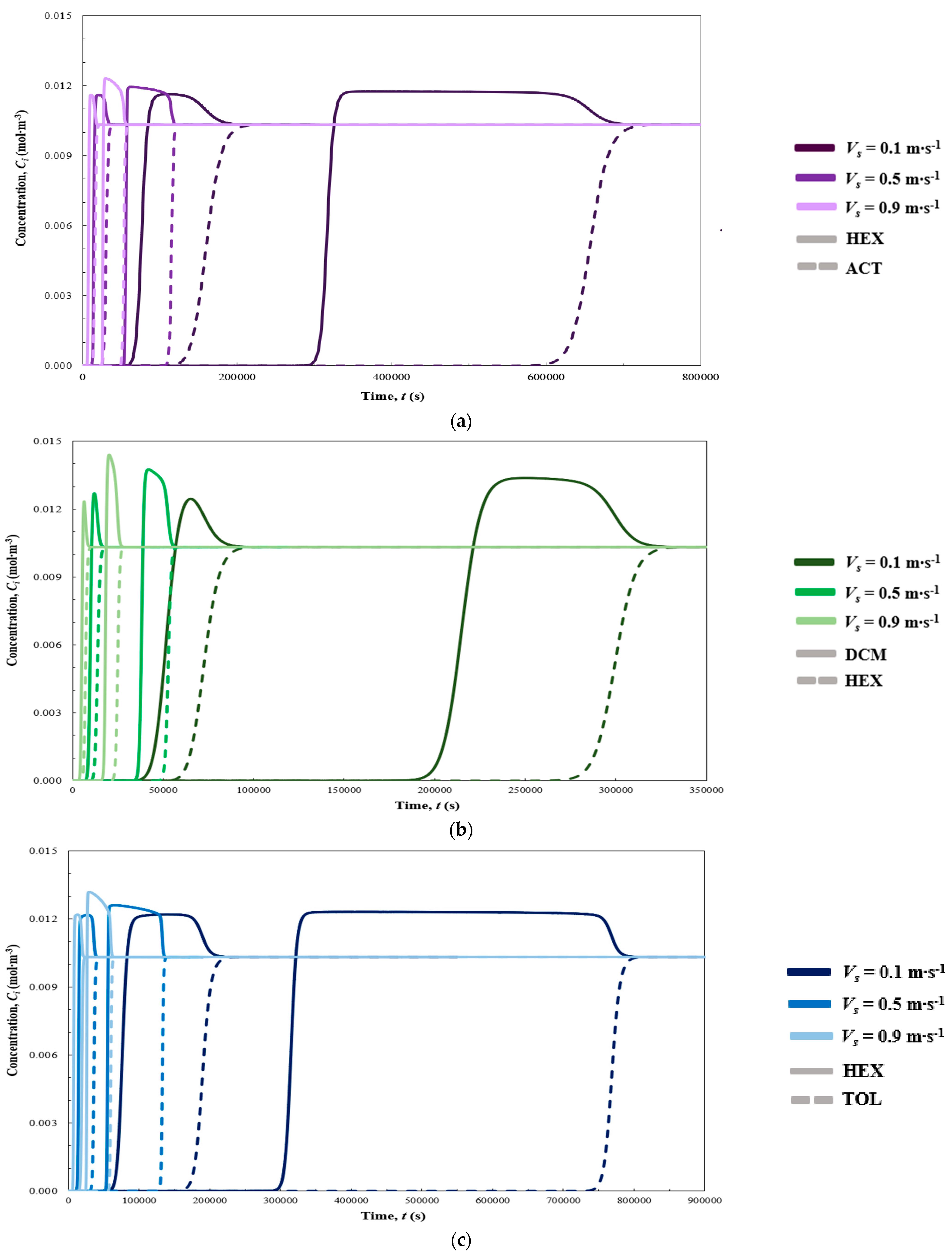
System	C0,i (ppm)	Dz,i (m2 s−1)	ΔHad,i (J mol−1)	Tin (K)	L (m)	Vs (m s−1)	qm (mol kg−1)	εb	kLDF (s−1)	b0 (m3 mol−1)	Figures
HEX-ACT	250	0.68∙10−3	51,100	300	0.25, 1	0.1	7.060	0.38	8.45∙10−5	1.96∙10−8	Figure 2 and Figure 3
	250	0.52∙10−3	50,000				3.801		1.66∙10−4	2.35∙10−8
HEX-ACT	250	1.07∙10−3	51,100	300	0.25, 1	0.5	7.060	0.38	8.45∙10−5	1.96∙10−8	Figure 2 and Figure 3
	250	0.91∙10−3	50,000				3.801		1.66∙10−4	2.35∙10−8
HEX-ACT	250	1.47∙10−3	51,100	300	0.25, 1	0.9	7.060	0.38	8.45∙10−5	1.96∙10−8	Figure 2 and Figure 3
	250	1.31∙10−3	50,000				3.801		1.66∙10−4	2.35∙10−8
HEX-DCM	250	0.67∙10−3	40,000	300	0.25, 1	0.1	4.510	0.38	2.32∙10−4	7.41∙10−7	Figure 2 and Figure 3
	250	0.52∙10−3	50,000				3.801		1.55∙10−4	2.35∙10−8
HEX-DCM	250	1.07∙10−3	40,000	300	0.25, 1	0.5	4.510	0.38	2.32∙10−4	7.41∙10−7	Figure 4 and Figure 5
	250	0.91∙10−3	50,000				3.801		1.55∙10−4	2.35∙10−8
HEX-DCM	250	1.46∙10−3	40,000	300	0.25, 1	0.9	4.510	0.38	2.32∙10−4	7.41∙10−7	Figure 4 and Figure 5
	250	1.31∙10−3	50,000				3.801		1.55∙10−4	2.35∙10−8
HEX-TOL	250	0.54∙10−3	45,500	300	0.25, 1	0.1	4.610	0.38	5.36∙10−5	4.06∙10−7	Figure 4 and Figure 5
	250	0.52∙10−3	50,000				3.801		1.91∙10−4	2.35∙10−8
HEX-TOL	250	0.93∙10−3	45,500	300	0.25, 1	0.5	4.610	0.38	5.36∙10−5	4.06∙10−7	Figure 4 and Figure 5
	250	0.91∙10−3	50,000				3.801		1.91∙10−4	2.35∙10−8
HEX-TOL	250	1.33∙10−3	45,500	300	0.25, 1	0.9	4.610	0.38	5.36∙10−5	4.06∙10−7	Figure 4 and Figure 5
	250	1.31∙10−3	50,000				3.801		1.91∙10−4	2.35∙10−8

). The adsorbent (beaded activated carbon, BAC) thus has a BET area of 1390 m² g⁻¹, a micropore volume of 0.51 cm³ g⁻¹, and a total pore volume of 0.57 cm³ g⁻¹ [22]. This study shows plots for two bed lengths (L = 0.25 m vs. L = 1 m) and three velocities (V_s = 0.1, 0.5, 0.9 m s⁻¹).

The PDAE system [34] is solved via a second-order orthogonal collocation method on finite elements in the gPROMS Process 2.0.0 environment [35]. The SRADAU DASolver (fully implicit, variable-time step Runge–Kutta method) is used, with Wilke’s viscosity equation; gas density is computed via mixing rules from pure compound data [36,37,38].

Table 2. Main structural and thermal parameter values of the systems.

System	C0,i (ppm)	ρb (kg m−3)	D (m)	Tin (K)	εp	dp (m)	Cpp (J kg−1 K−1)	Cpg (J kg−1 K−1)	kez (W m−1 K−1)	ho (W m−2 K−1)	hint (W m−2 K−1)	kw (W m−1 K−1)	x (m)	Figures
HEX-ACT	250	606	0.0152	300	0.56	0.00075	706.7	1014	0.13	9.05	9.05	14.2	0.001	Figure 2 and Figure 3
	250
HEX-ACT	250	606	0.0152	300	0.56	0.00075	706.7	1014	0.39	32.75	32.82	14.2	0.001	Figure 2 and Figure 3
	250
HEX-ACT	250	606	0.0152	300	0.56	0.00075	706.7	1014	0.66	52.33	52.52	14.2	0.001	Figure 2 and Figure 3
	250
HEX-DCM	250	606	0.0152	300	0.56	0.00075	706.7	1013	0.13	9.04	9.05	14.2	0.001	Figure 2 and Figure 3
	250
HEX-DCM	250	606	0.0152	300	0.56	0.00075	706.7	1013	0.39	32.74	32.81	14.2	0.001	Figure 2 and Figure 3
	250
HEX-DCM	250	606	0.0152	300	0.56	0.00075	706.7	1013	0.66	52.32	52.50	14.2	0.001	Figure 4 and Figure 5
	250
HEX-TOL	250	606	0.0152	300	0.56	0.00075	706.7	1014	0.13	9.06	9.06	14.2	0.001	Figure 4 and Figure 5
	250
HEX-TOL	250	606	0.0152	300	0.56	0.00075	706.7	1014	0.39	32.80	32.87	14.2	0.001	Figure 4 and Figure 5
	250
HEX-TOL	250	606	0.0152	300	0.56	0.00075	706.7	1014	0.66	52.41	52.60	14.2	0.001	Figure 4 and Figure 5
	250

summarizes key structural (column and adsorbent) and thermal parameters.

Figure 2. Breakthrough curves at L = 0.25 m and L = 1 m for (a) HEX-ACT (b) HEX-DCM (c) HEX-TOL.

Figure 2. Breakthrough curves at L = 0.25 m and L = 1 m for (a) HEX-ACT (b) HEX-DCM (c) HEX-TOL.

Figure 3. Temperature trajectories for: (a) HEX-ACT, (b) HEX-DCM, (c) HEX-TOL.

Figure 3. Temperature trajectories for: (a) HEX-ACT, (b) HEX-DCM, (c) HEX-TOL.

Figure 4. Breakthrough metrics for all case studies: (a–c) HEX-ACT, (d–f) HEX-DCM, (g–i) HEX-TOL.

Figure 4. Breakthrough metrics for all case studies: (a–c) HEX-ACT, (d–f) HEX-DCM, (g–i) HEX-TOL.

Figure 5. Bed design metrics for the (a) HEX-ACT, (b) HEX-DCM, (c) HEX-TOL mixtures.

Figure 5. Bed design metrics for the (a) HEX-ACT, (b) HEX-DCM, (c) HEX-TOL mixtures.

3. Results

3.1. Dynamic Simulation Results

The adsorption of three binary VOC mixtures (with air as the carrier gas) was examined at two bed lengths (L = 0.25, 1 m) and three superficial velocities (V_s = 0.1, 0.5, 0.9 m s⁻¹). The breakthrough curves, depicting each component’s concentration at the column outlet over time, are presented in Figure 2, and key breakthrough metrics are summarized in

Table 3. Key breakthrough metrics for the HEX-ACT binary mixture.

	Vs (m s−1)	t5% (s)	t95% (s)	t105% (s)	$\mathit{\Delta }{\mathit{t}}_{5\mathit{\%}}^{95\mathit{\%}}$ (s)	$\mathit{\Delta }{\mathit{t}}_{5\mathit{\%}}^{105\mathit{\%}}$ (s)	Tmax (K)	ΔP (kPa)	Figure 2 and Figure 3
L = 0.25 m
ACT	0.1	135,185	186,806	-	51,622	-	295.80	0.91	Figure 2a and Figure 3a
HEX		66,240	82,722	167,489	-	101,249
ACT	0.5	26,858	34,048	-	7190	-	296.33	6.26	Figure 2a and Figure 3a
HEX		12,801	15,504	31,357	-	18,556
ACT	0.9	13,617	18,349	-	4732	-	296.58	15.15	Figure 2a and Figure 3a
HEX		6448	8292	16,517	-	10,069
L = 1 m
ACT	0.1	622,722	689,812	-	67,089	-	295.26	3.75	Figure 2a and Figure 3a
HEX		303,888	323,394	666,333	-	362,445
ACT	0.5	111,102	118,558	-	7457	-	295.40	28.41	Figure 2a and Figure 3a
HEX		54,223	56,818	115,936	-	61,714
ACT	0.9	50,841	55,686	-	4846	-	295.55	77.92	Figure 2a and Figure 3a
HEX		25,375	26,999	53,942	-	28,567

,

Table 4. Key breakthrough metrics for the HEX-DCM binary mixture.

	Vs (m s−1)	t5% (s)	t95% (s)	t105% (s)	$\mathsf{\Delta }{\mathit{t}}_{5\mathit{\%}}^{95\mathit{\%}}$ (s)	$\mathsf{\Delta }{\mathit{t}}_{5\mathit{\%}}^{105\mathit{\%}}$ (s)	Tmax (K)	ΔP (kPa)	Figure 2 and Figure 3
L = 0.25 m
DCM	0.1	42,484	55,960	80,433	-	37,949	295.80	0.93	Figure 2b and Figure 3b
HEX		62,155	84,074	-	21,919	-
DCM	0.5	8404	10,517	14,999	-	6595	296.32	6.37	Figure 2b and Figure 3b
HEX		11,961	15,695	-	3734	-
DCM	0.9	4243	5606	8039	-	3796	296.57	15.15	Figure 2b and Figure 3b
HEX		6018	8550	-	2532	-
L = 1 m
DCM	0.1	199,347	219,975	309,736	-	110,389	295.20	3.75	Figure 2b and Figure 3b
HEX		283,768	314,348	-	30,579	-
DCM	0.5	36,236	38,780	54,261	-	18,025	295.36	28.41	Figure 2b and Figure 3b
HEX		50,523	54,470	-	3948	-
DCM	0.9	17,133	18,586	25,943	-	8811	295.52	77.92	Figure 2b and Figure 3b
HEX		23,409	26,467	-	3059	-

and

Table 5. Key breakthrough metrics for the HEX-TOL binary mixture.

	Vs (m s−1)	t5% (s)	t95% (s)	t105% (s)	$\mathsf{\Delta }{\mathit{t}}_{5\mathit{\%}}^{95\mathit{\%}}$ (s)	$\mathsf{\Delta }{\mathit{t}}_{5\mathit{\%}}^{105\mathit{\%}}$ (s)	Tmax (K)	ΔP (kPa)	Figure 2 and Figure 3
L = 0.25 m
TOL	0.1	174,107	206,227	-	32,120	-	295.77	0.93	Figure 2c and Figure 3c
HEX		66,179	81,570	197,352	-	131,173
TOL	0.5	33,483	38,827	-	5344	-	296.31	6.37	Figure 2c and Figure 3c
HEX		12,864	15,170	37,191	-	24,327
TOL	0.9	16,902	20,982	-	4079	-	296.56	15.15	Figure 2c and Figure 3c
HEX		6505	8102	19,644	-	13,139
L = 1 m
TOL	0.1	752,898	784,410	-	31,512	-	295.27	3.75	Figure 2c and Figure 3c
HEX		302,704	320,280	775,966	-	473,262
TOL	0.5	130,518	134,963	-	4445	-	295.42	28.41	Figure 2c and Figure 3c
HEX		53,973	56,165	133,890	-	79,917
TOL	0.9	58,333	61,930	-	3597	-	295.59	77.92	Figure 2c and Figure 3c
HEX		25,170	26,488	60,772	-	35,602

and Figure 3. Breakthrough onset time is calculated as the time required for the outlet concentration to reach 5% of the final concentration. Breakthrough completion times (t_95%–t_105%) are calculated as the time required for the outlet concentration to reach 95% of the final concentration for the strongly adsorbing component and 105% of the final concentration for the component that exits the bed first. Each colour corresponds to a superficial velocity and includes two sets of lines (one for L = 0.25 m, another for L = 1 m).

Figure 2a presents the breakthrough curves for the mixture of hexane–acetone (HEX-ACT). Breakthrough curves represent the concentration at the column outlet vs. time. It becomes apparent that the greater the superficial velocity, the sooner the breakthrough onset time. For each colour, the first set of lines, corresponding to L = 0.25 m, demonstrates a faster breakthrough onset compared to the second set of lines of the same colour representing the case of L = 1 m. It is interesting to note that for L = 1 m, the peak concentration of hexane increases with increasing superficial velocity.

For a bed length of L = 0.25 m, for V_s = 0.1 m s⁻¹_, the breakthrough onset time of hexane is 66,240 s, which is 81% later compared to the case of V_s = 0.5 m s⁻¹_, and 90% later compared to V_s = 0.9 m s⁻¹. At L = 1 m, for V_s = 0.1 m s⁻¹_, the breakthrough onset time of hexane is 303,888 s, which is 82% later compared to V_s = 0.5 m s⁻¹_, and 92% later compared to V_s = 0.9 m s⁻¹. For V_s = 0.1 m s⁻¹, the breakthrough onset of hexane at L = 0.25 m is 78% earlier vs. L = 1 m; for V_s = 0.5 m s⁻¹_, it occurs 76% earlier and for V_s = 0.9 m s⁻¹ it is 75% earlier.

The breakthrough onset time of acetone at L = 0.25 m is t_5% = 135,185 s, which is 80% later compared to V_s = 0.5 m s⁻¹ and an entire order of magnitude later compared to the case of V_s = 0.9 m s⁻¹. For a velocity of V_s = 0.1 m s⁻¹_, the breakthrough onset of acetone is 78% sooner at L = 0.25 m compared to L = 1 m, while for V_s = 0.5 m s⁻¹_, acetone’s onset is 76% earlier for a bed length of L = 0.25 m vs. L = 1 m, and for V_s = 0.9 m s⁻¹ it is 73% earlier.

Moreover, Figure 2a also provides information regarding the breakthrough duration of the HEX-ACT mixtures. For a bed length of L = 0.25 m, the breakthrough duration of hexane is 101,249 s for velocity V_s = 0.1 m s⁻¹_, which is 82% longer than for V_s = 0.5 m s⁻¹_, and one order of magnitude longer than for V_s = 0.9 m s⁻¹. For V_s = 0.1 m s⁻¹_, the breakthrough duration of hexane is 72% shorter for L = 0.25 m compared to L = 1 m, and for a higher velocity of V_s = 0.5 m s⁻¹, it is 70% shorter for L = 0.25 m, compared to L = 1 m. Finally, for V_s = 0.9 m s⁻¹_, the breakthrough duration for hexane is 65% quicker for L = 0.25 vs. 1 m.

For acetone, at L = 0.25 m, the breakthrough duration at V_s = 0.1 m s⁻¹ is 51,622 s, which is 86% longer compared to V_s = 0.5 m s⁻¹ and 91% longer compared to V_s = 0.9 m s⁻¹. For V_s = 0.1 m s⁻¹_, the breakthrough duration for acetone is 23% shorter for L = 0.25 m compared to L = 1 m. For V_s = 0.5 m s⁻¹_, the breakthrough duration for acetone is 4% shorter for L = 0.25 m compared to L = 1 m, and for V_s = 0.9 m s⁻¹ it is 2% shorter for L = 0.25 vs. 1 m.

Table 3 also presents key temperature and pressure drop metrics for the ACT-HEX mixtures. Specifically, the highest temperature peak is observed for L = 0.25 m at T_max = 296.58 K for V_s = 0.9 m s⁻¹, and the lowest T_max = 295.26 K for V_s = 0.1 m s⁻¹, but for a 1 m long column. Pressure drop, as predicted by Ergun’s equation and as expected, is lowest for the smallest velocity (V_s = 0.1 m s⁻¹) at 0.91 kPa for L = 0.25 m and 3.75 kPa for L = 1 m.

Table 3, Table 4 and Table 5 present breakthrough metrics for all three binary mixtures explored.

Figure 2b presents breakthrough curves for the hexane–dichloromethane (HEX-DCM) mixture. Key metrics are summarized in Table 4 and illustrated in Figure 4d–f. At L = 0.25 m, for V_s = 0.1 m s⁻¹_, the breakthrough onset time of hexane is 62,155 s, which is 81% later compared to V_s = 0.5 m s⁻¹ and 90% later compared to V_s = 0.9 m s⁻¹. At L = 1 m, for V_s = 0.1 m s⁻¹_, the breakthrough onset time of hexane is 283,768 s, which is 82% later compared to V_s = 0.5 m s⁻¹ and 92% later compared to V_s = 0.9 m s⁻¹. For V_s = 0.1 m s⁻¹_, the breakthrough onset of hexane at L = 0.25 m is 78% earlier compared to the largest bed (L = 1 m), for V_s = 0.5 m s⁻¹ it occurs 76% earlier, and for V_s = 0.9 m s⁻¹ even earlier (74%).

The breakthrough onset time of DCM at L = 0.25 m, for V_s = 0.1 m s⁻¹, is 42,484 s, which is 80% later compared to V_s = 0.5 m s⁻¹_, and one order of magnitude later compared to V_s = 0.9 m s⁻¹. For V_s = 0.1 m s⁻¹_, the breakthrough onset of DCM occurs 79% sooner at L = 0.25 m compared to the largest VOC bed (L = 1 m), while for the mid-value velocity of V_s = 0.5 m s⁻¹ the DCM onset occurs 77% earlier, and for V_s = 0.9 m s⁻¹ it occurs 75% earlier.

The breakthrough duration of the HEX-DCM mixtures can also be deduced from Figure 2b. At L = 0.25 m, the breakthrough duration of hexane is 21,949 s for V_s = 0.1 m s⁻¹_, which is 83% longer than for V_s = 0.5 m s⁻¹ and 88% longer than for V_s = 0.9 m s⁻¹. For V_s = 0.1 m s⁻¹, the breakthrough duration of hexane is 28% shorter for L = 0.25 m compared to L = 1 m, and for V_s = 0.5 m s⁻¹ it is 5% shorter for L = 0.25 m compared to L = 1 m. Finally, for V_s = 0.9 m s⁻¹, the breakthrough duration for hexane is 17% quicker for L = 0.25 vs. 1 m.

For dichloromethane, at L = 0.25 m, the breakthrough duration at V_s = 0.1 m s⁻¹ is 37,949 s, which is 83% longer compared to V_s = 0.5 m s⁻¹ and one order of magnitude longer compared to V_s = 0.9 m s⁻¹. For V_s = 0.1 m s⁻¹_, the dichloromethane breakthrough duration is 63% shorter for a short vs. long bed (L = 0.25 vs. 1 m). For V_s = 0.5 m s⁻¹_, the breakthrough duration for DCM is again 63% shorter, but for V_s = 0.9 m s⁻¹ it is clearly shorter (57%).

Temperature and pressure drops for HEX-DCM mixtures are given in Table 4. The highest temperature peak is for L = 0.25 m (T_max = 296.57 K for V_s = 0.9 m s⁻¹), and the lowest T_max = 295.20 K is for V_s = 0.1 m s⁻¹, for a long bed (L = 1 m). Pressure drop is lowest for the smallest velocity (V_s = 0.1 m s⁻¹) at 0.93 kPa for L = 0.25 m, but high (3.75 kPa) for L = 1 m.

Figure 2c presents breakthrough curves for hexane–toluene (HEX-TOL) mixtures. Key metrics are summarized in Table 5 and Figure 4g–i. For L = 0.25 m at V_s = 0.1 m s⁻¹_, the hexane breakthrough onset is at 66,179 s, 81% later compared to V_s = 0.5 m s⁻¹ and 90% later compared to V_s = 0.9 m s⁻¹. For L = 1 m and V_s = 0.1 m s⁻¹, the hexane breakthrough onset is at 302,704 s, which is 82% later compared to V_s = 0.5 m s⁻¹ and 92% later compared to V_s = 0.9 m s⁻¹. Thus, for V_s = 0.1 m s⁻¹_, hexane breakthrough onset at L = 0.25 m is 78% earlier compared to L = 1 m. For V_s = 0.5 m s⁻¹ it is 76% earlier and for V_s = 0.9 m s⁻¹ it is 74% earlier.

For toluene, the breakthrough onset time at L = 0.25 m, for V_s = 0.1 m s⁻¹_, is 174,107 s, which is 81% later compared to V_s = 0.5 m s⁻¹ and 90% later compared to V_s = 0.9 m s⁻¹. For V_s = 0.1 m s⁻¹, toluene breakthrough onset occurs 77% sooner for L = 0.25 m compared to L = 1 m; for V_s = 0.5 m s⁻¹, it occurs 74% earlier at L = 0.25 m compared to L = 1 m, and for V_s = 0.9 m s⁻¹, it occurs 71% earlier.

Breakthrough duration metrics of HEX-TOL mixtures are seen in Figure 2c. For L = 0.25 m, the breakthrough duration of hexane is 131,173 s for V_s = 0.1 m s⁻¹_, which is 81% longer than for V_s = 0.5 m s⁻¹_, and an order of magnitude longer than for V_s = 0.9 m s⁻¹. For V_s = 0.1 m s⁻¹_, the breakthrough duration of hexane is 72% shorter for L = 0.25 m compared to L = 1 m, and for V_s = 0.5 m s⁻¹, it is 70% shorter for L = 0.25 m compared to L = 1 m. For V_s = 0.9 m s⁻¹_, the hexane breakthrough duration is 63% shorter for L = 0.25 m compared to 1 m.

For toluene, at L = 0.25 m, the breakthrough duration at V_s = 0.1 m s⁻¹ is 32,120 s, which is 83% longer compared to V_s = 0.5 m s⁻¹ and 87% longer compared to V_s = 0.9 m s⁻¹. For V_s = 0.1 m s⁻¹, the breakthrough duration for toluene is 2% longer for L = 0.25 m compared to L = 1 m. For V_s = 0.5 m s⁻¹_, the breakthrough duration for TOL is again 17% longer for L = 0.25 m compared to L = 1 m, and for V_s = 0.9 m s⁻¹, it is 12% longer for L = 0.25 vs. 1 m.

Temperature and pressure drop metrics for the HEX-TOL mixtures are presented in Table 5. Specifically, the highest temperature peak is observed for the shortest VOC bed (L = 0.25 m) at T_max = 296.56 K for V_s = 0.9 m s⁻¹, and the lowest T_max = 295.27 K for V_s = 0.1 m s⁻¹ in the largest (1 m long) VOC capture column. Pressure drop, as expected, is lowest for the smallest velocity (V_s = 0.1 m s⁻¹), at 0.93 kPa for L = 0.25 m and 3.75 kPa for L = 1 m.

Figure 4 summarizes the key breakthrough metrics we have obtained from dynamic simulations for all binary systems, at three superficial velocities (V_s = 0.1, 03, 0.5 m s⁻¹) and two bed lengths (L = 0.25, 1 m). Evidently, the lowest crude inlet feed velocity (V_s = 0.1 m s⁻¹) corresponds to the longest breakthrough onset times, which increase with the increasing superficial velocity case studies. Breakthrough onset hence occurs earlier for the laboratory-scale VOC capture column (L = 0.25 m) than for an industrial-size bed (L = 1 m).

Breakthrough duration, though, also displays binary mixture-specific characteristics which cannot be predicted a priori on the basis of molecular structure or polarity alone. For the hexane–acetone (HEX-ACT) mixture, both components’ breakthrough durations are shorter for the laboratory-scale column and decrease with increasing superficial velocity. For the hexane–dichloromethane (HEX-DCM) mixture, the same trends hold for both components. These simulation observations agree with experimental studies which have explored the adsorption of polar gases on similar (not the same) adsorbents [39,40].

For the hexane–toluene (HEX-TOL) mixture, however, there is a clear difference: the foregoing trend holds true for hexane breakthrough duration, but not for the toluene one. Toluene exhibits shorter breakthrough durations in the larger (industrial-size) than in the shorter (laboratory-size) VOC capture bed, which is also shown to further decrease with increasing superficial velocity. The adsorption and desorption behaviour and kinetics of toluene, specifically, shows interesting complexity with pore structure variation [41,42], which has not been investigated for the case of mixtures and industrial-size columns.

The non-isothermal, multicomponent adsorption PDAE model we have employed also provides insight into spatiotemporal temperature variations useful in design [34,35].

Sharp, early (t < 100 s) temperature peaks increase with increasing superficial velocity, particularly for short beds (L = 0.25 m), but more complex thermal behaviour (multiple, wider, and later peaks) is seen for lower superficial velocities and longer beds (L = 1 m). Hexane (HEX) is part of all mixtures, and temperature peaks are very close (twins) for dichloromethane (DCM), less close (clearly distinct in most trajectories) for acetone (ACT), and farthest apart in time for toluene (TOL), for which they are also evidently asymmetric.

3.2. Bed Design Results

One of the key parameters to consider upon designing an industrial adsorption column for emissions abatement is the breakthrough onset time (t_5%); shedding light on how it is impacted by various mixtures and operating conditions is of great importance to stakeholders. A new metric, called normalised time (denoted as: t*) is hereby introduced in order to quantify the effect of bed length (and scale-up) on breakthrough onset time. Normalised time (t*) is the ratio of breakthrough onset time over column length.

The adsorption behaviour of said mixtures of hexane–acetone (HEX-ACT), hexane–dichloromethane (HEX-DCM), and hexane–toluene (HEX-TOL) is examined for four bed lengths (L = 0.25, 0.50, 0.75, 1 m) and six superficial velocities of industrial crude gas feed into the adsorption bed (V_s = 0.1, 0.2, 0.3, 0.5, 0.7, 0.9 m s⁻¹) under the same conditions reported in Table 1 and Table 2, to determine the correlation between breakthrough onset time, column length, and velocity (

Table 6. Breakthrough onset times for superficial velocities 0.2, 0.3, and 0.7 m s⁻¹ for Figure 5.

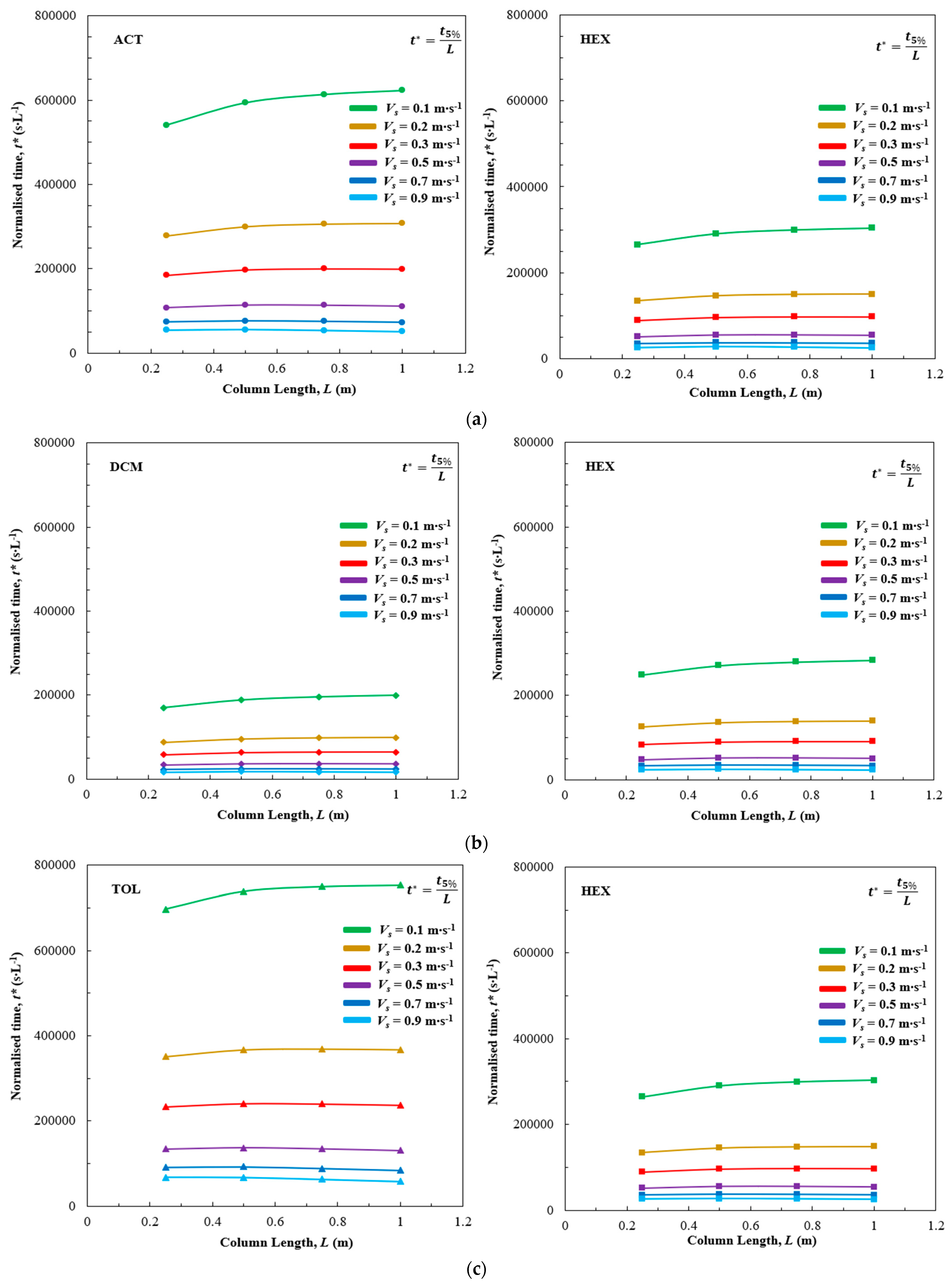
t5% (s)
Vs (m s−1)	L (m)	HEX	ACT	HEX	DCM	HEX	TOL
0.2	0.25	33,597	69,512	31,469	21,845	33,619	87,770
	0.50	72,803	149,991	67,930	47,647	72,683	183,365
	0.75	111,529	229,683	104,243	73,573	111,228	276,469
	1	149,461	307,725	139,910	99,142	148,910	367,014
0.3	0.25	22,161	46,164	20,741	14,503	22,228	58,203
	0.50	47,818	98,816	44,587	31,444	47,801	120,317
	0.75	72,796	150,078	67,946	48,156	72,679	179,796
	1	96,970	199,526	90,643	64,544	96,557	236,853
0.7	0.25	8726	18,384	8145	5738	8785	22,865
	0.50	18,534	38,348	17,196	12,233	18,560	46,203
	0.75	27,520	56,359	25,515	18,312	27,459	66,563
	1	35,669	72,429	33,080	23,925	35,472	84,252

), to develop a potential adsorption bed design tool.

Figure 5 shows the normalised time metrics vs. column length for all components and superficial velocities. Figure 5a refers to the hexane–acetone mixture, Figure 5b to the hexane–dichloromethane mixture, and Figure 5c to the hexane–toluene mixture. Common trends emerge for all systems considered: the weakly adsorbing mixture component demonstrates lower values of normalised time due to earlier breakthrough onset.

Furthermore, our simulation results show that with increasing superficial velocity, normalised time metrics not only shift to lower values, but also demonstrate a smaller gap (hence a smaller change) in breakthrough onset. There is a velocity range for which there is an optimal trade-off among process energy consumption (turbines required to maintain pressure), cost savings from more efficient bed use (longer periods between adsorbent changeovers/regeneration), and process recipe (crude feed volume to bed constraints).

Another trend is observed pertaining to length scale-up and velocities. Specifically, at high superficial velocities, the normalised time values reported for increasing bed lengths tend to follow a straight line, thus indicating an analogous relationship between length scale-up and breakthrough onset times. However, a different story unfolds for lower superficial velocity values, where it is observed that the normalised time increases with increasing bed length until a certain length, after which it evidently stabilises to a plateau. This observation gives rise to the conclusion that in combination with an optimal velocity range, there is also an optimal adsorption bed size (length) range, which allows for prolonged bed usage between adsorbent regenerations (later breakthrough onset) and avoids a large, costly column without operational benefit.

4. Conclusions

Volatile organic compound (VOC) emissions are inevitable by-products of upstream pharmaceutical manufacturing [43,44]. Due to potentially toxic effects on the environment and human health, an ever-increasing focus on regulations aims to ensure and safeguard their limited, controlled release into the atmosphere. Adsorption is an established industrial VOC emissions abatement technology, capable of processing large gas waste volumes with trace pollutant concentrations. Nevertheless, due to mixture complexity and feed pattern irregularity, adsorption operation is often suboptimal, thus increasing total cost.

The present paper demonstrates the application of a validated, multicomponent, non-isothermal adsorption model to investigate the effect of superficial velocity and adsorption bed length on multicomponent VOC mixture adsorption. We studied the breakthrough behaviour of binary VOC mixtures (hexane–acetone, hexane–dichloromethane, and hexane–toluene) with air as a carrier gas through beaded activated carbon [22,42] for four bed lengths ranging from laboratory to industrial scale (L = 0.25, 0.50, 0.75, 1 m) and six superficial velocities (V_s = 0.1, 0.2, 0.3, 0.5, 0.7, 0.9 m s⁻¹). Breakthrough results are shown only for L = 0.25 m and L = 1 m (min-max) at V_s = 0.1, 0.5, 0.9 m s⁻¹ (min-mid-max). Finally, normalised time is introduced and plotted as a useful metric (breakthrough onset over bed length ratio) for all cases considered, to assist column design decision-making.

This detailed breakthrough behaviour study reveals remarkable trends between the said VOCs and process parameters. Specifically, for all simulation cases considered, the latest breakthrough onset times occur for the lowest superficial velocity and longest column. Breakthrough durations have mixture-specific characteristics. For the hexane–acetone and hexane–dichloromethane mixtures (and for hexane within the hexane–toluene mixture), breakthrough durations are shorter for the laboratory-scale bed and decrease with increasing superficial velocity. For toluene, a shorter duration is observed in the industrial-scale bed, which decreases with increasing superficial velocity. Temperature peaks are highest for the shortest VOC beds at the largest superficial velocity, while the smallest pressure drops occur in the short-column, low-superficial velocity scenarios.

Moreover, the concept of normalised time is proposed as an adsorption column utilisation tool. Specifically, the increasing proximity of the plot lines in Figure 4 with increasing superficial velocity indicates that there is a velocity range enabling the balance among process energy consumption (for compressors maintaining the pressure), cost savings from increased bed efficiency (hence less frequent need for adsorbent regeneration), and plant emissions constraints. In tandem with an optimal velocity range, there seems to also be an optimal bed length range which would allow for prolonged bed usage between adsorbent regenerations (later breakthrough onset) while minimising the capital (and operational) cost associated with constructing and running a very long adsorption column. These findings pave the way for better VOC emissions control in the pharma industry, with higher process efficiency, at lower cost and smaller environmental footprint.

References

- Gonzalez Pena, O.I.; Lopez Zavala, M.A.; Cabral Ruelas, H. Pharmaceuticals market, consumption trends and disease incidence are not driving the pharmaceutical research on water and wastewater. Int. J. Environ. Res. Public Health 2021, 18, 2532. [Google Scholar] [CrossRef] [PubMed]
- David, J.C.; Constable, C.J.-G.; Henderson, R.K. Perspective on solvent use in the pharma industry. Org. Process Res. Dev. 2007, 11, 133–137. [Google Scholar] [CrossRef]
- Henderson, R.K.; Jiménez-González, C.; Constable, D.J.C.; Alston, S.R.; Inglis, G.G.A.; Fisher, G.; Sherwood, J.; Binks, S.P.; Curzons, A.D. Expanding GSK’s solvent selection guide—Embedding sustainability into solvent selection starting at medicinal chemistry. Green Chem. 2011, 13, 854–862. [Google Scholar] [CrossRef]
- Sheldon, R.A. The E factor: Fifteen years on. Green Chem. 2007, 9, 1273–1283. [Google Scholar] [CrossRef]
- UK Government, Department of Environment, Food & Rural Affairs. Emissions of Air Pollutants in The UK—Non-Methane Volatile Organic Compounds (NMVOCs). 2023. Available online: https://www.gov.uk/government/statistics/emissions-of-air-pollutants/emissions-of-air-pollutants-in-the-uk-non-methane-volatile-organic-compounds-nmvocs (accessed on 11 September 2023).
- Ma, J.W.; Li, L. VOC emitted by biopharmaceutical industries: Source profiles, health risks, and secondary pollution. J. Environ. Sci. 2024, 135, 570–584. [Google Scholar] [CrossRef] [PubMed]
- Simayi, M.; Shi, Y.Q.; Xi, Z.Y.; Ren, J.; Hini, G.; Xie, S.D. Emission trends of industrial VOCs in China since the clean air action and future reduction perspectives. Sci. Total Environ. 2022, 826, 153994. [Google Scholar] [CrossRef]
- Delage, F.P.P.; Le Cloirec, P. Mass transfer and warming during adsorption of high concentrations of VOCs on an activated carbon bed: Experimental and theoretical analysis. Environ. Sci. Technol. 2000, 34, 4816–4821. [Google Scholar] [CrossRef]
- Ruthven, D.M. Principles of Adsorption and Adsorption Processes; John Wiley & Sons Inc.: Hoboken, NJ, USA, 1984. [Google Scholar]
- Suzuki, M. Adsorption Engineering; Elsevier Science Publishers: Amsterdam, The Netherlands, 1990. [Google Scholar]
- Huang, H.; Haghighat, F.; Blondeau, P. Volatile organic compound (VOC) adsorption on material: Influence of gas phase concentration, relative humidity and VOC type. Indoor Air 2006, 16, 236–247. [Google Scholar] [CrossRef] [PubMed]
- Laskar, I.I.; Hashisho, Z.; Phillips, J.H.; Anderson, J.E.; Nichols, M. Modeling the effect of relative humidity on adsorption dynamics of volatile organic compound onto activated carbon. Environ. Sci. Technol. 2019, 53, 2647–2659. [Google Scholar] [CrossRef]
- Zheng, C.; Kang, K.; Xie, Y.C.; Yang, X.L.; Lan, L.; Song, H.; Han, H.; Bai, S.P. Dynamic adsorption behavior of 1.1.1.2-tetrafluoroethane (R134a) on activated carbon beds under different humidity and moisture levels. Sep. Purif. Technol. 2024, 329, 124851. [Google Scholar] [CrossRef]
- Cosnier, F.; Celzard, A.; Furdin, G.; Bégin, D.; Marêché, J.F. Influence of water on the dynamic adsorption of chlorinated VOCs on active carbon: Relative humidity of the gas phase versus pre-adsorbed water. Adsorpt. Sci. Technol. 2006, 24, 215–228. [Google Scholar] [CrossRef]
- Yao, X.L.; Liu, Y.; Li, T.; Zhang, T.T.; Li, H.L.; Wang, W.; Shen, X.B.; Qian, F.; Yao, Z.L. Adsorption behavior of multicomponent volatile organic compounds on a citric acid residue waste-based activated carbon: Experiment and molecular simulation. J. Hazard. Mater. 2020, 392, 122323. [Google Scholar] [CrossRef] [PubMed]
- Cheng, T.; Jiang, Y.; Zhang, Y.; Liu, S. Prediction of breakthrough curves for adsorption on activated carbon fibers in a fixed bed. Carbon 2004, 42, 3081–3085. [Google Scholar] [CrossRef]
- Li, Z.; Li, Y.; Zhu, J. Straw-based activated carbon: Optimization of the preparation procedure and performance of volatile organic compounds adsorption. Materials 2021, 14, 3284. [Google Scholar] [CrossRef]
- Fu, J.; Jin, C.; Zhang, J.; Wang, Z.; Wang, T.; Cheng, X.; Ma, C.; Chen, H. Pore structure and VOCs adsorption characteristics of activated coke powders derived via one-step rapid pyrolysis activation method. Asia-Pac. J. Chem. Eng. 2020, 15, e2503. [Google Scholar] [CrossRef]
- Xiao, J.S.; Peng, Y.Z.; Bénard, P.; Chahine, R. Thermal effects on breakthrough curves of pressure swing adsorption for hydrogen purification. Int. J. Hydrogen Energy 2016, 41, 8236–8245. [Google Scholar] [CrossRef]
- Jee, J.G.; Kim, M.B.; Lee, C.H. Adsorption characteristics of hydrogen mixtures in a layered bed: Binary, ternary, and five-component mixtures. Ind. Eng. Chem. Res. 2001, 40, 868–878. [Google Scholar] [CrossRef]
- Moe, W.M.; Collins, K.L.; Rhodes, J.D. Activated carbon load equalization of gas-phase toluene: Effect of cycle length and fraction of time in loading. Environ. Sci. Technol. 2007, 41, 5478–5484. [Google Scholar] [CrossRef]
- Tefera, D.T.; Lashaki, M.J.; Fayaz, M.; Hashisho, Z.; Philips, J.H.; Anderson, J.E.; Nichols, M. Two-dimensional modeling of volatile organic compounds adsorption onto beaded activated carbon. Environ. Sci. Technol. 2013, 47, 11700–11710. [Google Scholar] [CrossRef]
- Tefera, D.T.; Hashisho, Z.; Philips, J.H.; Anderson, J.E.; Nichols, M. Modeling competitive adsorption of mixtures of volatile organic compounds in a fixed-bed of beaded activated carbon. Environ. Sci. Technol. 2014, 48, 5108–5117. [Google Scholar] [CrossRef]
- Tzanakopoulou, V.E.; Pollitt, M.; Castro-Rodriguez, D.; Costa, A.; Gerogiorgis, D.I. Dynamic modelling, simulation and theoretical performance analysis of Volatile Organic Compound (VOC) abatement systems in the pharma industry. Comput. Chem. Eng. 2023, 174, 108248. [Google Scholar] [CrossRef]
- Tzanakopoulou, V.E.; Pollitt, M.; Castro-Rodriguez, D.; Gerogiorgis, D.I. Dynamic model validation and simulation of acetone–toluene and benzene–toluene systems for industrial Volatile Organic Compound (VOC) abatement. Ind. Eng. Chem. Res. 2024, 63, 7281–7299. [Google Scholar] [CrossRef] [PubMed]
- Tzanakopoulou, V.E.; Narasinghe, K.; Pollitt, M.; Castro-Rodriguez, D.; Gerogiorgis, D.I. Dynamic simulation and analysis of dichloromethane-acetone, dichloromethane-trichloromethane and dichloromethane-toluene VOC mixture abatement systems under transient feed conditions. Comput. Chem. Eng. 2024, 187, 108713. [Google Scholar] [CrossRef]
- Sircar, S.; Hufton, J.R. Why does the Linear Driving Force model for adsorption kinetics work? Adsorpt.-J. Int. Adsorpt. Soc. 2000, 6, 137–147. [Google Scholar] [CrossRef]
- Krishna, R.; van Baten, J.M. Investigating the validity of the Bosanquet formula for estimation of diffusivities in mesopores. Chem. Eng. Sci. 2012, 69, 684–688. [Google Scholar] [CrossRef]
- Knox, J.C.; Ebner, A.D.; LeVan, M.D.; Coker, R.F.; Ritter, J.A. Limitations of breakthrough curve analysis in fixed-bed adsorption. Ind. Eng. Chem. Res. 2016, 55, 4734–4748. [Google Scholar] [CrossRef]
- Giraudet, S.P.; Pré, P.; Le Cloirec, P. Modeling the temperature dependence of adsorption equilibirums of VOCs onto activated carbons. J. Environ. Eng. 2010, 136, 103–111. [Google Scholar] [CrossRef]
- Chuang, C.L.; Chiang, P.C.; Chang, E.E. Modeling VOCs adsorption onto activated carbon. Chemosphere 2003, 53, 17–27. [Google Scholar] [CrossRef]
- Shim, W.G.; Lee, J.W.; Moon, H. Equilibrium and fixed-bed adsorption of n-hexane on activated carbon. Sep. Sci. Technol. 2003, 38, 3905–3926. [Google Scholar] [CrossRef]
- Talmoudi, R.; AbdelJaoued, A.; Chahbani, M.H. Dynamic study of VSA and TSA processes for VOCs removal from air. Int. J. Chem. Eng. 2018, 2018, 2316827. [Google Scholar] [CrossRef]
- Angelopoulos, P.M.; Gerogiorgis, D.I.; Paspaliaris, I. Mathematical modeling and process simulation of perlite grain expansion in a vertical electrical furnace. Appl. Math. Model. 2014, 38, 1799–1822. [Google Scholar] [CrossRef]
- Akinlabi, C.O.; Gerogiorgis, D.I.; Georgiadis, M.C.; Pistikopoulos, E.N. Modelling, design and optimisation of a hybrid PSA-membrane gas separation process. Comput.-Aided Chem. Eng. 2007, 24, 363–370. [Google Scholar] [CrossRef]
- National Institute of Standards and Technology (NIST). Thermophysical Properties of Fluid Systems. 2023. Available online: https://webbook.nist.gov/chemistry/fluid/ (accessed on 11 September 2023).
- Coker, A.K. Physical Properties of Liquids and Gases. In Ludwig’s Applied Process Design for Chemical & Petrochemical Plants, 4th ed.; Coker, A.K., Ed.; Gulf Professional Publishing: Houston, TX, USA, 2007; pp. 103–132. [Google Scholar]
- Gerogiorgis, D.I.; Barton, P.I. Steady-state optimization of a continuous pharmaceutical process. Comput.-Aided Chem. Eng. 2009, 27, 927–932. [Google Scholar] [CrossRef]
- Kim, S.J.; Cho, S.Y.; Kim, T.Y. Adsorption of chlorinated volatile organic compounds in a fixed bed of activated carbon. Korean J. Chem. Eng. 2002, 19, 61–67. [Google Scholar] [CrossRef]
- Tsai, J.H.; Chiang, H.M.; Huang, G.Y.; Chiang, H.L. Adsorption characteristics of acetone, chloroform and acetonitrile on sludge-derived adsorbent, commercial granular activated carbon and activated carbon fibers. J. Hazard. Mater. 2008, 154, 1183–1191. [Google Scholar] [CrossRef]
- Yang, X.; Yi, H.H.; Tang, X.L.; Zhao, S.Z.; Yang, Z.Y.; Ma, Y.Q.; Feng, T.C.; Cui, X.X. Behaviors and kinetics of toluene adsorption-desorption on activated carbons with varying pore structure. J. Environ. Sci. 2018, 67, 104–114. [Google Scholar] [CrossRef] [PubMed]
- Izquierdo, M.T.; Martínez de Yuso, A.; Rubio, B.; Pino, M.R. Conversion of almond shell to activated carbons: Methodical study of the chemical activation based on an experimental design and relationship with their characteristics. Biomass Bioenergy 2011, 35, 1235–1244. [Google Scholar] [CrossRef]
- Jolliffe, H.G.; Gerogiorgis, D.I. Technoeconomic optimisation and comparative environmental impact evaluation of continuous crystallisation and antisolvent selection for artemisinin recovery. Comput. Chem. Eng. 2017, 103, 218–232. [Google Scholar] [CrossRef]
- Jolliffe, H.G.; Gerogiorgis, D.I. Process modelling, design and technoeconomic evaluation for continuous paracetamol crystallisation. Comput. Chem. Eng. 2018, 118, 224–235. [Google Scholar] [CrossRef]