A Dynamic Assessment Model of Distributed Photovoltaic Carrying Capacity Based on Improved DeepLabv3+ and Game-Theoretic Combination Weighting

Abstract

The traditional carrying capacity assessment method fails to effectively quantify the difference in spatial distribution of rooftop photovoltaic (PV) resources and ignores the temporal fluctuation of PV output and load demand, as well as the temporal and spatial matching characteristics of sources and loads. This leads to problems such as a disconnect between the assessment and the actual grid acceptance capacity and insufficient dynamic adaptability. In response to the above issues, this paper proposes a dynamic assessment model for distributed photovoltaic carrying capacity based on the combination of improved DeepLabv3+ and game-theoretic weighted assignment. First, the DeepLabv3+ model was improved by integrating the Efficient Channel Attention (ECA) mechanism and the strip pooling (SP) module to enhance roof recognition accuracy. Ablation experiments showed that the mIoU increased to 77.53%, 6.29% higher than the original model. The simulation results in the summer scenario demonstrated that, with the optimal coordination of STMF and scene scoring, the comprehensive carrying coefficient reached 0.73. Next, a photovoltaic carrying capacity evaluation system was established, considering the source, grid, and load perspectives, with dynamic evaluation using a game-theory-based weighting method. Finally, a comprehensive carrying coefficient was introduced, accounting for the spatiotemporal match between photovoltaic output and load, leading to the development of a distributed photovoltaic carrying capacity model. The case study results show that, in summer, due to the optimal coordination of STMF and scene scoring, the comprehensive carrying coefficient reaches 0.73. With a total PV access capacity of 6.48 MW, all node voltages remain within limits, verifying the model’s effectiveness in grid adaptability.

1. Introduction

In recent years, driven by China’s county-level distributed PV promotion policy and the falling cost of PV modules, rooftop PV systems have seen rapid growth. The dense deployment of distributed PV has become a major trend in distribution network development, pushing the traditional power system toward a high-renewable energy structure [1,2,3]. However, distributed PV output is highly random and volatile. Large-scale integration poses challenges to voltage stability, power quality, supply reliability, and the economic operation of the distribution network [4,5,6]. At the same time, with the overlap of renewable energy access and load-side uncertainties, the system faces high-dimensional uncertainty on both the generation and load sides, along with limited regulation capacity. Traditional evaluation methods based on deterministic assumptions or fixed boundaries struggle to reflect real operational conditions effectively [7,8].

To analyze the impact of large-scale distributed photovoltaic integration on distribution grid operation, research is increasingly focusing on developing a multi-objective evaluation system. Ref. [9] addresses the stability, economy, and flexibility of distribution network operation, establishing a multi-level carrying capacity evaluation system and converting the evaluation results into a comprehensive score using a combined weighting method. Ref. [10] proposes a multi-objective decision evaluation method for the new energy carrying capacity in distribution networks, aiming to develop a complete DG carrying capacity model. Ref. [11] creates a carrying capacity influence index, considering factors such as voltage over-limit, short-circuit current over-limit, and power quality, and determines the weights using an improved entropy weighting method. While these studies focus on the safe and stable operation of distribution systems, they do not quantitatively analyze the dynamic correlation between photovoltaic power and the spatiotemporal distribution of load.

To describe the grid’s capacity for new energy, the National Energy Administration introduced the concept of carrying capacity, which refers to the maximum amount of new energy that can be integrated without compromising the grid’s security and stability [12]. Ref. [13] addresses load uncertainty and proposes a two-layer programming method to determine the maximum access capacity of distributed power sources under voltage constraints. Ref. [14] presents an optimization method for the collaborative operation of medium- and low-voltage distribution networks, considering flexible interconnected distribution substations to ensure safe and stable operation. Ref. [15] examines the impact of distributed photovoltaic grid-connected capacity on network losses and establishes a new evaluation model for the carrying capacity of distributed photovoltaics in medium-voltage distribution networks. Ref. [16] introduces a two-layer optimization model for power system loss reduction, based on the collaborative optimization of ‘source-grid-load-storage’ to coordinate controllable distributed resources, reduce network losses, and ensure safe and economic operation. Ref. [17] considers constraints such as node voltage, line power flow, and power return to evaluate the carrying capacity of new energy in the power system. While these studies ensure the reliability of power system operation through strict safety constraints, they do not account for the variability of photovoltaic output and load uncertainty.

Many researchers have begun to introduce uncertainty modeling methods to further improve the accuracy of assessments. Ref. [18] fully accounts for renewable energy and load uncertainty, constructing typical scenarios to enhance the applicability of power system planning and dispatching. Ref. [19] generates typical scenarios for the combined operation of light intensity and load power and proposes an economic access capacity evaluation method that considers the appropriate levels of PV curtailment. Ref. [20] proposes a method to enhance the carrying capacity of distributed photovoltaic power by considering correlations. Ref. [21] introduces parameters to characterize photovoltaic and load uncertainties and, based on this, proposes a cluster zoning planning method with reliability considerations. Ref. [22] addresses both distributed power source and flexible resource scheduling uncertainties in distribution networks, suggesting an interval evaluation method for renewable energy carrying capacity. Refs. [23,24] propose an opportunity-constrained assessment method for the carrying capacity of integrated energy systems, factoring in the uncertainty and volatility of new energy. Refs. [25,26,27] present a two-stage optimal allocation method for integrated energy systems, considering photovoltaic uncertainty in the context of carbon trading. However, these methods inadequately address high-dimensional heterogeneous data, such as building characteristics and geographical information, when modeling and evaluating the photovoltaic capacity of distribution networks.

Considering the full potential of rooftop photovoltaics can significantly enhance the accuracy of capacity estimation. As a result, researchers have conducted studies to estimate the potential of rooftop PV systems. Ref. [28] estimates rooftop area and photovoltaic potential using population, building density, and land use data, determining the availability coefficient for representative buildings. Ref. [29] proposes a deep-learning-based method for rooftop PV resource assessment that combines and applies image segmentation techniques with a PV simulation component. It recognizes building roofs based on the Double Convolutional God Network model Double U-Net. Ref. [30] proposes a PV carrying capacity evaluation method based on the improved PSPNet and CRITIC methods.

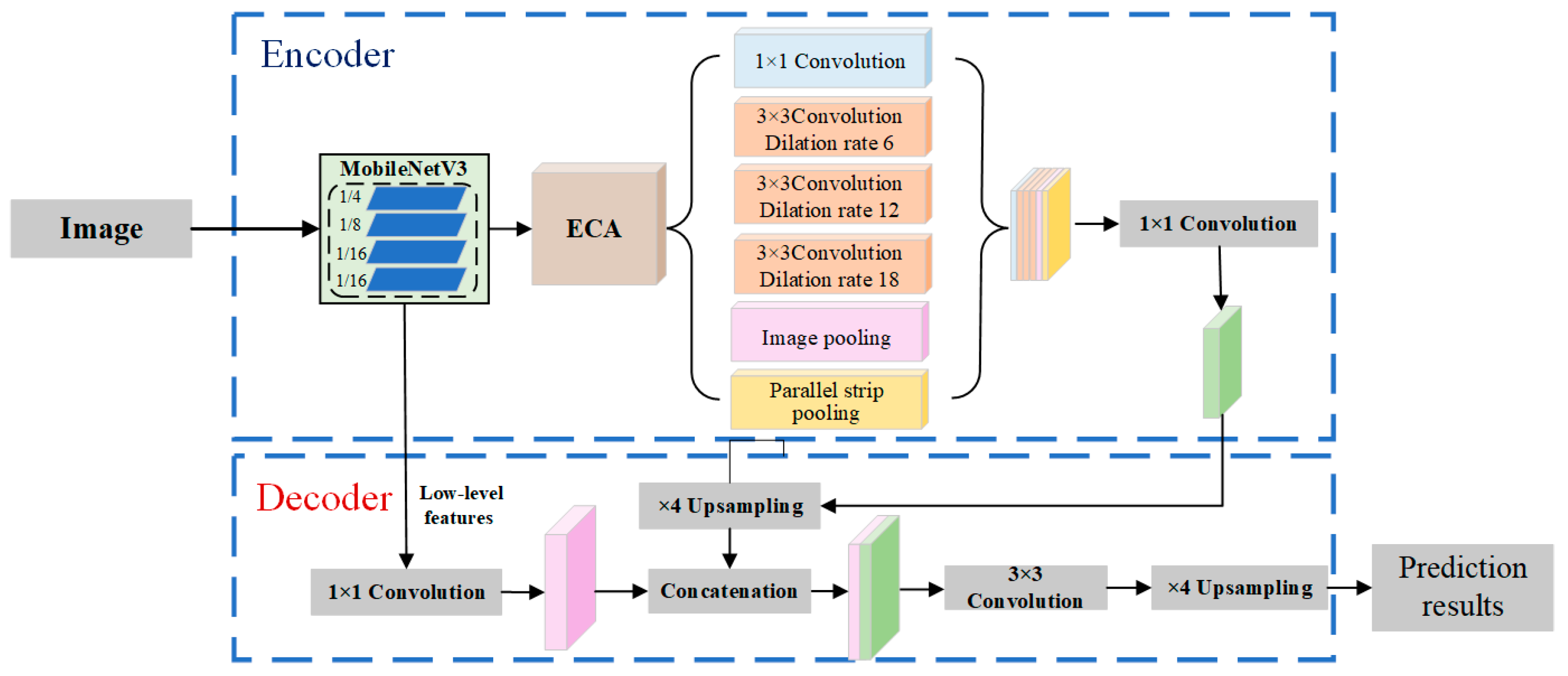
PSPNet’s pooling operation tends to lose spatial details and involves high computational cost. U-Net’s skip connections can introduce noise and have a limited receptive field. Ref. [31] added an encoder–decoder structure to DeepLabv3+, achieving better performance through dilated convolution and multi-scale feature fusion. However, this approach struggles with high-resolution images. Ref. [32] replaced DeepLabv3+’s backbone with MobileNetV2, using only the first eight layers to reduce computation. Dilated convolutions were applied in layers 7 and 8, with the stride of layer 7 set to one, which improved the segmentation accuracy. Although this model reduces the parameter count, its accuracy for complex and irregular targets remains limited. As shown in

Table 1. Comparison of existing methods.

Number	Reference	Core Methodology	Main Advantages	Limitations	Comparison of Innovations
1	[28]	A statistical model based on population and building density.	Requires minimal data; suitable for macro-level estimation.	Ignores structural details of buildings.	Lacks image-level analysis; results in low accuracy.
2	[29]	U-Net algorithm for rooftop extraction.	Achieves high-accuracy rooftop segmentation.	Skip connections may introduce noise and limit receptive field.	Skip connections are prone to noise and offer limited contextual awareness.
3	[30]	Improved PSPNet, grid data, and CRITIC method.	Multi-source data for comprehensive evaluation.	Pooling loses spatial details and increases computational complexity.	Pooling operations cause detail loss and are computation-intensive.
4	[31]	Deeplabv3+ (dilated convolution and multi-scale fusion)	Preserves details well and models long-range dependencies effectively.	Struggles with high-resolution image processing.	High computational cost for high-resolution images.
5	[32]	MobileNetV2 as the backbone network.	Low computational cost and faster segmentation.	Poor segmentation accuracy for complex targets.	Accuracy drops for complex and irregular targets.
6	This paper	Improved Deeplabv3+.	Lightweight, preserves details, and robust to noise.	Requires balance between lightweight design and adaptability to extreme scenarios.	MobileNetV3 for lightweight structure; ECA attention for enhanced feature focus; strip pooling for spatial detail refinement.

, to solve the problems of the above methods, we enhance DeepLabv3+ by introducing the MobileNetV3 backbone, the ECA attention mechanism, and ribbon pooling. These additions aim to improve recognition accuracy while keeping the model lightweight.

In summary, the current research on the carrying capacity of distribution networks has notable limitations. First, the traditional assessment methods do not fully account for the spatial distribution of rooftop photovoltaic potential, making it difficult for results to accurately reflect the actual operating conditions of the distribution system. Second, most existing studies focus on static analysis, overlooking the volatility and uncertainty of PV output and load under dynamic conditions, limiting the flexibility of system assessments.

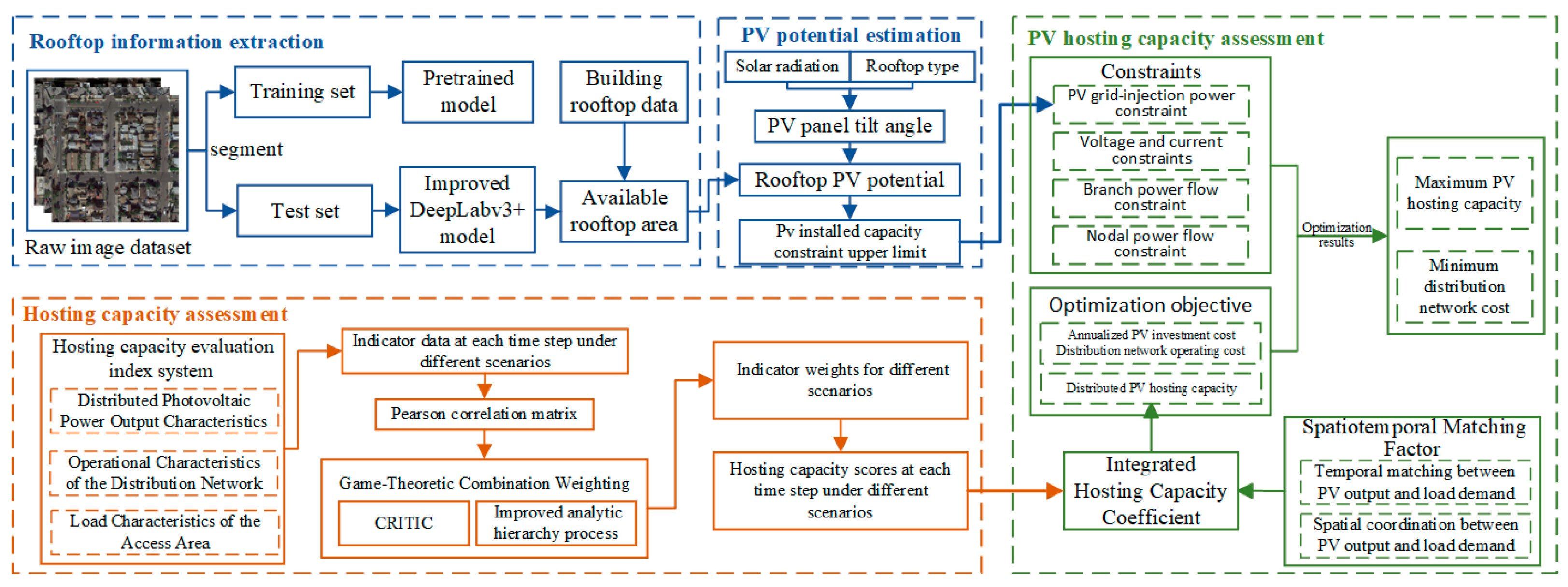
To address these challenges, this paper proposes a dynamic evaluation method for the carrying capacity of distributed PV systems in distribution networks. First, an improved DeepLabV3+ model is developed to identify and estimate rooftop PV potential. Second, an evaluation index system is designed, and a game-theory-based weighting method is introduced to support dynamic assessment. Finally, a comprehensive carrying coefficient is defined, and a carrying capacity evaluation model based on multi-source data is established.

2. Framework of Photovoltaic Carrying Capacity Assessment Model

As a key component of the electrical system, the distribution network ensures the reliable transmission of electricity from the source to various consumers. It supplies power to diverse load scenarios, including residential areas, industrial parks, and schools. Figure 1 illustrates the structure of a distribution network with a high proportion of integrated distributed photovoltaics.

To address the challenges posed by the large-scale integration of distributed PV systems, such as increased operational pressure on distribution networks, spatial decoupling, and the lack of spatiotemporal dynamics in traditional evaluation methods, this paper proposes a dynamic evaluation model framework that combines improved DeepLabv3+ and game-theoretic combination weighting, as shown in Figure 2. It evaluates the carrying capacity of the distribution network through multi-source data fusion, spatiotemporal dynamic correction, and multi-objective optimization.

(1)

A photovoltaic installed capacity calculation method based on the improved DeepLabv3+ model is proposed, considering high-dimensional heterogeneous data such as photovoltaic resources and building characteristics. This method accurately evaluates photovoltaic potential in different regions and provides reasonable constraints for PV access capacity.

(2)

The carrying capacity evaluation system is built from three aspects: photovoltaic output characteristics, distribution network operation characteristics, and load-side characteristics. The game-theoretic combination weighting method is used to evaluate the network’s safe operation under varying photovoltaic access and load change conditions.

(3)

The spatiotemporal matching correction factor is introduced to construct a comprehensive carrying coefficient and develop the distributed photovoltaic carrying capacity evaluation model. The model uses this coefficient to form the objective function, optimizing the photovoltaic carrying capacity configuration and enhancing the accuracy and applicability of the results.

3. Rooftop Photovoltaic Potential Measurement Method

3.1. Improved DeepLabv3+ Model

This paper proposes an improved DeepLabv3+ semantic segmentation algorithm, and its structure is shown in Figure 3. The improvement targets key issues in roof segmentation, such as detail loss, blurred edges, and poor long-range dependency modeling. First, MobileNetV3 is used as the backbone to enhance boundary detection accuracy and improve the extraction of small-target features while maintaining a lightweight structure and strong scene adaptability. Second, the ECA attention mechanism is embedded in both the backbone and the Atrous Spatial Pyramid Pooling (ASPP) module. It recalibrates channel responses to suppress redundant noise and enhance key features. This improves the efficiency of multi-scale feature extraction and reduces the number of model parameters. Additionally, the SP module is integrated in parallel with ASPP to address its limitations in detecting elongated, stripe-like structures. This enhances global context awareness along narrow directions and effectively mitigates spatial fragmentation. As a result, the segmentation of linear targets in urban and remote sensing images becomes more coherent. The improved model achieves balance between segmentation accuracy, edge detail, and detection speed.

3.1.1. MobileNetV3 Backbone Network

MobileNetV3’s unique Squeeze-and-Excitation (SE) module pools each channel of the input feature map to enhance the model’s representational power. The core of the squeeze stage is global average pooling (GAP), which compresses the spatial information of each channel into a scalar, capturing global context. This allows the model to assess the importance of each channel, improving both its representational ability and efficiency. The calculation formula is:

$$z_c={\displaystyle \frac{1}{H\times W}}{\displaystyle \sum _{i=1}^H{\displaystyle \sum _{j=1}^W{x}_{c,i,j}}}$$

(1)

where H is the height of the feature map, W is the width of the feature map, and z_c is the output value of the c-th channel after global average pooling.

The excitation stage redistributes the attention weights across channels to enhance the important features and suppress the irrelevant ones. It processes the compressed vector through two fully connected layers. The first layer reduces the feature dimension to extract more significant information, while the second layer maintains the same number of nodes as the number of channels in the input feature matrix. The resulting feature vectors from these layers provide the channel weights, which are applied to the original matrix. The calculation formula is:

$$\omega =\sigma 1\left(W_{1}z\right)$$

(2)

where σ1 is an activation function and W₁ is a fully connected weight matrix.

To achieve weighting processing for each channel, the generated channel weights are multiplied channel-by-channel with the original feature map.

$$Y_{i,j,c}=X_{i,j,c}\cdot {\omega }_c$$

(3)

where Y_i,j,c is the value of the c-th channel of the output feature map at position (i,j), X_i,j,c is the value of the c-th channel of the input feature map at position (i,j), and ω_c is the weight of the c-th channel generated after passing the excitation stage.

3.1.2. Efficient Channel Attention Mechanism

The ECA structure is a lightweight channel attention mechanism that enhances feature representation while reducing computational complexity and memory usage. It optimizes feature map expression in convolutional neural networks by calculating the interaction of information within each channel, allowing the model to focus on the most important channel features.

(1)

In the GAP stage, the input feature map is globally averaged. Specifically, the input feature map U ∈ R^H×W×C with dimensions (H, W, C) is reduced to (1, 1, C), where H, W, and C represent the height, width, and number of channels, respectively. The GAP operation then compresses the feature map from (H, W, C) to (1, 1, C).

(2)

We then calculate the adaptive convolution kernel size. An adaptive convolution kernel size is obtained by a fully connected layer for subsequent convolution operations.

$$k=\phi \left(c\right)={\left|{\displaystyle \frac{{\log }_2^c}{\gamma }}+{\displaystyle \frac{b}{\gamma }}\right|}_{odd}$$

(4)

where k is the kernel size; φ(c) is the mapping function; b is an adaptive convolutional kernel, which acts as a bias; and γ is the scaling factor for the global average pooling output.

The weight calculation involves applying the adaptive convolution kernel in a one-dimensional convolution operation to obtain adaptive weights for each channel in the feature map.

$$\omega =\sigma \left(Con{v}_k\left(y\right)\right)$$

(5)

where y is the input feature, σ is the activation function, and Conv_k is the one-dimensional convolution operation with a kernel size of k.

Feature weighting involves multiplying the normalized weights with the original input feature map, channel by channel, to obtain the weighted feature map. This operation enhances the model’s learning and improves the extraction of important features.

3.1.3. Strip Pooling

SP is a pooling method where a long strip-shaped core is applied along the spatial dimension. Banded pooling divides the current feature map into several banded regions based on specific rules. Standard pooling is then performed on each band, resulting in a set of smaller feature maps after pooling. Suppose the input feature is x ∈ R^H×W×C. When horizontal pooling with a 1 × W pooling kernel is applied, the output is a column vector of size H × 1 × C. The expression for this output is:

$$y_{c,i}^h={\displaystyle \frac{1}{W}}{\displaystyle \sum _{0\le j<W}{X}_{i,j,c}}$$

(6)

When vertical pooling is applied with a W × 1 pooling kernel, the output is a row vector of size 1 × W × C. The expression for this output is:

$$y_{c,i}^v={\displaystyle \frac{1}{H}}{\displaystyle \sum _{0\le i<H}{X}_{i,j,c}}$$

(7)

where i and j represent the pixel positions in the i-th row and j-th column of the feature map, respectivley.

3.2. Rooftop Photovoltaic Potential Measurement

The main roof types are flat, sloped, and arched roofs. Although arched roofs have a more complex shape, their structural curvature is typically smoother, similar to traditional sloped roofs. Therefore, for the purpose of calculation, arched roofs are simplified to sloped roofs. In this case, the photovoltaic panels are installed flat, with the tilt angle of the panels matching that of the roof.

The flat roof photovoltaic system adjusts the installation angle based on the region’s latitude, longitude, and surrounding obstructions to maximize solar radiation reception. The photovoltaic panels are installed facing south. When calculating the maximum radiation received at different tilt angles, assuming that scattered radiation is evenly distributed in space, the solar radiation intensity I_θ at a tilt angle θ is:

$$I_{\theta }=I_b\cdot \cos i+I_d\cdot {\displaystyle \frac{1+\cos \theta }{2}}$$

(8)

where I_b is direct radiation, i is the angle of solar incidence, and I_d is scattered radiation.

The total radiant energy Q_y received by the solar panels over the course of a year is:

$$Q_y={\displaystyle {\int }_{N=1}^{365}{\displaystyle {\int }_{T_{sr}}^{T_{ss}}{I}_{\theta }dT}}$$

(9)

where T_sr is the sunrise time and T_ss is the sunset time.

The formula for calculating the available roof area of a flat roof is:

$$S_{fg}={\displaystyle \frac{S_t\times B_1\times B_2\times F_f}{\cos \theta +\sin \theta \cdot \coth \cdot \cos \alpha }}$$

(10)

where S_fg represents the available roof area for a flat roof; F_f reflects the ratio of the flat roof area; B₁ is the roof correction coefficient considering the shadows of a chimney, antenna, and trees, which is generally set at 0.7; B₂ is the equipment correction factor, which considers the space occupied by equipment on the roof, and is generally assumed to be 0.9; S_t represents the total roof area; h is the solar altitude angle; and α is the solar azimuth angle.

The formula for calculating the available roof area of a sloped roof is:

$$S_{pg}={\displaystyle \frac{S_t\times B_1\times B_2\times F_p}{\cos {\theta }^{\prime }}}$$

(11)

where S_pg is the available roof area for the sloped roof, F_p represents the portion of the roof area occupied by the sloped roof, and θ′ is the tilt angle of the sloped roof photovoltaic panels.

The distributed photovoltaic installed capacity is calculated as follows:

$$P={\displaystyle \frac{(2S_{fg}+S_{pg})W_p}{2A}}$$

(12)

where A is the area of a single solar panel and W_p is the rated maximum output power of the photovoltaic panel under standard test conditions.

4. Dynamic Capacity Evaluation Model for Photovoltaic Integration

Following the principles of scientific accuracy, systematization, and quantification, key operational parameters are selected from the source, network, and load sides to create a multi-level, multi-dimensional evaluation index system. By applying an appropriate evaluation method, the dynamic score of the distribution network’s carrying capacity is obtained through a weighted summation of various network indicators.

4.1. Construction of a Multi-Level Evaluation System

This paper aims to assess the impact of a high proportion of distributed PV power on the operational performance of the distribution network. To reflect this impact, it establishes a carrying capacity evaluation system. The system takes the distribution network’s carrying capacity as the target layer. The criterion layer includes the distributed photovoltaic power output characteristics, the operational characteristics of the distribution network, and the load characteristics of the access area. The evaluation system is then quantitatively analyzed using a combined weighting method based on game theory. The constructed distribution network carrying capacity evaluation index system is shown in Figure 4.

4.1.1. Distributed Photovoltaic Power Output Characteristics

Since photovoltaic power generation is highly influenced by environmental factors such as light intensity and temperature, its volatility and uncertainty may cause many problems in distribution network operation. Therefore, it is essential to establish a scientifically sound and reasonable index system for quantitative analysis, based on the inherent characteristics of photovoltaic power generation.

(1) Local Photovoltaic Consumption Rate

The local photovoltaic consumption rate is the proportion of PV power in the distribution network that can be locally consumed by the loads as a percentage of the total power generated. It is expressed as:

$$\mu ={\displaystyle \frac{{\displaystyle \sum _{t=1}^T({\chi }_t{P}_{pv,t}+{\delta }_t{P}_{load,t})}}{{\displaystyle \sum _{t=1}^T{P}_{pv,t}}}}\times 100\%$$

(13)

where χ_t and δ_t are Boolean variables used to represent the size relationship between P_pv,t and P_load,t, with the condition that χ_t + δ_t = 1, when P_pv,t > P_load,t, δ_t = 1, otherwise, δ_t = 0; P_pv,t represents the active power output within the distribution network area; and P_load,t represents the load demand.

(2) Photovoltaic Output Volatility

The volatility of photovoltaic power measures the range of variation in its output. In this case, it is calculated using the standard deviation.

$$\Delta P_{PV}\left(t\right)=\sqrt{{\displaystyle \frac{1}{N}}{\displaystyle \sum _{i=1}^N{\left(P_{PV}\left(t_i\right)-\stackrel{-}{P_{PV}}\right)}^2}}$$

(14)

$${\sigma }_{PV}={\displaystyle \frac{\Delta P_{pv}}{\stackrel{-}{P_{PV}}}}\times 100\%$$

(15)

where σ_PV is the photovoltaic output volatility and P_PV(t_i) is the photovoltaic power generation at time t_i.

(3) Photovoltaic Penetration Rate

The photovoltaic penetration rate represents the proportion of photovoltaic power in the total load of the distribution system over a given operating cycle. It indicates the degree of saturation of the installed photovoltaic capacity within the distribution system.

$$APPR={\displaystyle \frac{1}{T}}{\displaystyle \sum _{t=1}^T\frac{{\displaystyle \sum _{i=1}^N{P}_{PV,i,t}}}{P_t}\times 100\%}$$

(16)

where P_PV,i,t represents the PV power at node i in the distribution system at time t.

4.1.2. Operational Characteristics of the Distribution Network

The integration of photovoltaic power may lead to issues such as voltage deviation, power flow fluctuations, and energy loss. Therefore, it is essential to establish appropriate evaluation indicators from the perspective of power system operation, which aids in the quantitative analysis of the impact of photovoltaic integration on distribution system performance.

(1) Voltage Deviation Rate

The voltage deviation rate refers to the proportion of the deviation between the node voltage in the distribution system and the rated voltage.

$$R_{\Delta U}={\displaystyle \frac{1}{N}}{\displaystyle \frac{1}{T}}{\displaystyle \sum _{i=1}^N{\displaystyle \sum _{t=1}^T\frac{\left|U_N-U_{i,t}\right|}{U_N}}}$$

(17)

where N is the total number of nodes, T is the system operation duration, U_N is the rated voltage, and U_i,t is the node voltage at node i in the system at time t.

(2) Power Flow Mismatch Degree

The degree of power flow mismatch refers to the ratio of the difference between the transmitted power and the average power on the distribution system’s transmission line to the line’s maximum transmitted power.

$$Q_{\Delta P,line}={\displaystyle \frac{1}{N_l}}{\displaystyle \frac{1}{T}}{\displaystyle \sum _{i=1}^{N_l}{\displaystyle \sum _{t=1}^T\frac{\left|P_{l,i,t}-P_{l,ave,t}\right|}{P_{l,\max }}}}$$

(18)

where N_l is the total number of lines, P_l,i,t is the transmitted power on branch i at time t, P_l,ave,t is the average transmitted power of the line at time t, and P_l,max is the maximum transmitted power of the line.

(3) Network Loss Rate

The network loss rate refers to the proportion of energy lost due to factors such as line impedance and electrical equipment during the transmission of electricity in the distribution network. It is a key indicator of the transmission efficiency of the power system.

$$R_{loss}={\displaystyle \frac{1}{T}}{\displaystyle \sum _{t=1}^T\frac{P_{loss,t}}{P_{c,t}}}$$

(19)

where P_loss,t is the total loss during the distribution network transmission process at time t and P_c,t is the total power transmitted by the distribution network at time t.

4.1.3. Load Characteristics of the Access Area

Load characteristics influence both the consumption capacity and the regulation potential of PV output on the load side. It is essential to develop an index system that quantitatively evaluates load characteristics from a load-side perspective.

(1) Load Utilization Rate

The load utilization rate reflects how effectively the system uses the available load capacity. A higher utilization rate indicates better load demand fulfillment and increased load-side revenue, thereby improving system economics. It is calculated as follows:

$$L_e={\displaystyle \frac{P_L}{P_s}}\times 100\%$$

(20)

where P_L represents the actual total load supplied and P_s denotes the maximum load demand.

(2) Net Load Fluctuation

Net load fluctuation indicates the rate of change in the distribution system’s net load over time within a given operating cycle.

$$ALFR={\displaystyle \frac{1}{T}}{\displaystyle \sum _{t=1}^T\frac{\left|P_t-P_{t-1}\right|}{P_t}\times 100\%}$$

(21)

where P_t represents the net load at time t and P_{t − 1} represents the net load at time t − 1.

(3) Maximum Load Imbalance Degree

The maximum load imbalance measures the ratio of the maximum and minimum values of the actual load to the total load over a specified time range.

$$F_d={\displaystyle \frac{P_{\max }-P_{\min }}{P_{\max }}}\times 100\%$$

(22)

where P_max is the maximum load value and P_min is the minimum load value.

4.2. Game-Theoretic Combination Weighting

To address the limitations of single weighting methods and derive more objective and reasonable standard weights, this paper proposes a game-theoretic combined weighting approach. This results in a more comprehensive evaluation of the system’s carrying capacity.

4.2.1. Index Normalization

To eliminate dimensional effects and enable consistent measurement across all data, the indicators are standardized to form a normalized matrix. For n evaluation objects and m evaluation indicators, the indicator matrix is defined as follows:

$$X=\left[\begin{array}{ccc}{x}_{11}& \dots & x_{1n}\\ ⋮& \ddots & ⋮\\ x_{m1}& \dots & x_{mn}\end{array}\right]$$

(23)

Processing for positive indicators is conducted as follows:

$$x_{ij}^{\prime }={\displaystyle \frac{x_{ij}-\min \left(x_i\right)}{\max \left(x_i\right)-\min \left(x_i\right)}}$$

(24)

Processing for negative indicators is conducted as follows:

$$x_{ij}^{\prime }={\displaystyle \frac{\max \left(x_i\right)-x_{ij}}{\max \left(x_i\right)-\min \left(x_i\right)}}$$

(25)

We also calculate the Pearson correlation coefficient matrix for all indicators. The closer the absolute value is to 1, the stronger the linear correlation between two variables. Values near 0 indicate little to no linear relationship.

$$r_{ij}={\displaystyle \frac{{\displaystyle {\sum }_{k=1}^n\left(x_{ik}^{\prime }-\stackrel{-}{x_i^{\prime }}\right)\left(x_{jk}^{\prime }-\stackrel{-}{x_j^{\prime }}\right)}}{\sqrt{{{\displaystyle {\sum }_{k=1}^n\left(x_{ik}^{\prime }-\stackrel{-}{x_i^{\prime }}\right)}}^2{{\displaystyle {\sum }_{k=1}^n\left(x_{jk}^{\prime }-\stackrel{-}{x_j^{\prime }}\right)}}^2}}}$$

(26)

where x_ik′ and x_jk′ represent the values of the i-th and j-th indicators for the k-th evaluation object, respectivley.

4.2.2. Improved Analytic Hierarchy Process

The Improved Analytic Hierarchy Process (AHP) is a decision-making method that integrates both qualitative and quantitative analysis. However, the construction of pairwise comparison matrices is often influenced by expert judgment or personal bias. To enhance objectivity, this paper proposes a method that uses the Pearson correlation matrix between indicators to construct the comparison matrix. Here, let R denote the resulting Pearson correlation coefficient matrix:

$$R=\left[\begin{array}{cccc}1& r_{12}& \dots & r_{1m}\\ r_{21}& 1& \dots & r_{2m}\\ ⋮& ⋮& \ddots & ⋮\\ r_{m1}& r_{m2}& \dots & 1\end{array}\right]$$

(27)

To construct the judgment matrix, the Pearson correlation coefficient matrix is transformed using the following formula:

$${\mu }_{ij}={\displaystyle \frac{1}{1-r_{ij}^2}}$$

(28)

$$W=\left[\begin{array}{cccc}1& {\mu }_{12}& \dots & {\mu }_{1m}\\ {\mu }_{21}& 1& \dots & {\mu }_{2m}\\ ⋮& ⋮& \ddots & ⋮\\ {\mu }_{m1}& {\mu }_{m2}& \dots & 1\end{array}\right]$$

(29)

when i = j, μ_ij = 1; and when i ≠ j, μ_ij is the off-diagonal weight value determined by the Pearson correlation coefficient, with μ_ij × μ_ji = 1.

The weights of each index are determined by evaluating the matrix, solving for its eigenvectors and eigenvalues, and performing a consistency test.

$$CR={\displaystyle \frac{{\lambda }_{\max }-m}{\left(m-1\right)RI}}$$

(30)

where RI is the Random Consistency Index. If CR < 1, the matrix is considered to have acceptable consistency, and the corresponding eigenvector can be used as the weight vector.

4.2.3. CRITIC

CRITIC is an objective weighting method based on data variability and conflict. The information capacity C_j reflects the amount of information contained in the j-th indicator. A higher value of C_j indicates the greater weight of that indicator in the evaluation system. The calculation formula is as follows:

$$C_j=P_j\times A_j=\sqrt{{\displaystyle \frac{{\displaystyle \sum _{i=1}^m{\left(x_{ij}^{\prime }-\overline{x_j^{\prime }}\right)}^2}}{n-1}}}\cdot {\displaystyle \sum _{i=1}^m\left(1-r_{ij}\right)}$$

(31)

where P_j represents data variability. The higher its value is, the more volatile the data will be, and the higher the weight will be. A_j represents indicator conflict, where a higher value implies lower conflict among the indicators, resulting in a lower weight. r_ij is the correlation coefficient between evaluation indicators i and j. The formula for calculating the objective weight of the j-th indicator is as follows:

$$w_j=C_j/{\displaystyle \sum _{j=1}^m{C}_j}$$

(32)

4.2.4. Game-Theoretic Approaches

If the weight vector w₁, obtained through the subjective weighting method, is considered to be one side of the game, and the weight vector w₂, determined by the CRITIC method, is the other side, then the optimal combined weight is the one that brings both sides to equilibrium. At equilibrium, the deviation between the combined weight and both w₁ and w₂ should be minimized. Here, let α₁ and α₂ be the distribution coefficients for ω₁ and ω₂, and let w be the resulting linear combination. The calculation formula is as follows:

$$w={\alpha }_1{w}_1^T+{\alpha }_2{w}_2^T$$

(33)

Based on game theory principles, an objective function is defined to minimize the deviation between the combined weight w and the individual weights ω₁ and ω₂. The goal is to determine the optimal combination coefficients that balance both weighting methods. The objective function and corresponding constraints are as follows:

$$\left\{\begin{array}{c}\min \left({‖{\alpha }_1{w}_1^T+{\alpha }_2{w}_2^T-w_1^T‖}_2+{‖{\alpha }_1{w}_1^T+{\alpha }_2{w}_2^T-w_2^T‖}_2\right)\\ s.t.{\alpha }_1+{\alpha }_2=1,{\alpha }_1\ge 0,{\alpha }_2\ge 0\end{array}\right.$$

(34)

According to the principle of differentiation, to minimize Equation (34), the derivative conditions for each variable are linearly combined and expanded, resulting in the following expression:

$$\left[\begin{array}{cc}{w}_1{w}_1^T& w_1{w}_2^T\\ w_2{w}_1^T& w_2{w}_2^T\end{array}\right]\left[\begin{array}{c}{\alpha }_1\\ {\alpha }_2\end{array}\right]=\left[\begin{array}{c}{w}_1{w}_1^T\\ w_2{w}_2^T\end{array}\right]$$

(35)

The optimal combined weight is:

$$\left\{\begin{array}{c}\begin{array}{l}w*={\alpha }_1^{*}{w}_1^T+{\alpha }_2^{*}{w}_2^T\\ {\alpha }_1^{*}=\left|{\alpha }_1\right|/\left(\left|{\alpha }_1\right|+\left|{\alpha }_2\right|\right)\end{array}\\ {\alpha }_2^{*}=\left|{\alpha }_2\right|/\left(\left|{\alpha }_1\right|+\left|{\alpha }_2\right|\right)\end{array}\right.$$

(36)

5. Distributed Photovoltaic Carrying Capacity Model and Solution

In distribution networks with high PV penetration, traditional capacity assessment methods face limitations, as they fail to accurately reflect the system’s operational characteristics near safety constraint boundaries after large-scale renewable integration. To address this issue, this paper proposes a comprehensive carrying coefficient and develops a distributed photovoltaic hosting capacity model to quantify the coordination between distribution network operation and renewable energy integration capacity.

5.1. Integrated Hosting Capacity Coefficient Modeling

The carrying capacity coefficient serves as a core indicator for evaluating the operational health of distribution networks following photovoltaic integration. It is calculated through a weighted aggregation of multiple factors, including PV output characteristics, network operation status, and load profiles. A spatiotemporal matching factor (STMF) is introduced as a dynamic weighting adjustment, reflecting the alignment between PV generation and load demand in both time and space. By quantifying source–load synergy, STMF enables dynamic correction of the hosting capacity evaluation.

5.1.1. Temporal Matching Degree

The Temporal Matching Degree (TMD) quantifies the correlation between PV output and load demand over time. It incorporates a time-weighting coefficient to emphasize the influence of matching performance during different time periods. It is defined as follows:

$$\left\{\begin{array}{l}TMD={\displaystyle \sum _{t=1}^T\gamma \left(t\right)\frac{\left(P_{PV}\left(t\right)-{\overline{P}}_{PV}\right)\left(P_{Load}\left(t\right)-{\overline{P}}_{Load}\right)}{{\sigma }_{PV}\cdot {\sigma }_{Load}}}\\ \gamma \left(t\right)=P_{Load}\left(t\right)/{\displaystyle \sum _{t=1}^T{P}_{Load}\left(t\right)}\end{array}\right.$$

(37)

where P_PV(t) and P_Load(t) represent the photovoltaic output and load power at time t, respectivley, and σ_PV and σ_Load denote the standard deviations of the photovoltaic output and load power, respectivley.

5.1.2. Spatial Matching Degree

The Spatial Matching Degree (SMD) measures the alignment between PV output and load demand across different regions. It reflects the deviation in the local supply–demand ratio and is defined as follows:

$$SMD=1-{\displaystyle \frac{1}{N}}{\displaystyle \sum _{i=1}^N\left|\frac{C_{PV,i}/C_{PV,total}}{D_{Load,i}/D_{Load,total}}-1\right|}$$

(38)

where N is the number of nodes in the distribution network, C_PV,i represents the PV hosting capacity at node i, D_Load,i is the load demand at node i, C_PV,total denotes the total PV hosting capacity, and D_Load,total is the total load demand.

5.1.3. Spatiotemporal Matching Factor

The calculation formula for the weighted fusion of temporal and spatial matching is as follows:

$$STMF=\beta \cdot TMD+\left(1-\beta \right)\cdot SMD$$

(39)

where β represents the spatiotemporal weighting coefficient.

The calculation formula for the comprehensive carrying capacity coefficient is as follows:

$$G={\displaystyle \sum _{i=1}^{N_{index}}{w}_i{g}_i}\cdot \left(1+\alpha \cdot STMF\right)/100$$

(40)

where N_index is the number of distribution network carrying capacity indicators, w_i represents the weight of the i-th indicator, g_i is the score of the i-th indicator, and α denotes the matching degree gain coefficient.

5.2. Objective Function

In constructing the objective function, a dual-objective optimization approach is adopted, fully accounting for both technical and economic feasibility. On one hand, the comprehensive hosting capacity of distributed PV systems is maximized to enhance the integration of renewable energy. On the other hand, economic factors, such as PV investment, operation and maintenance costs, and penalties for curtailed PV output, are considered with the goal of minimizing the full life-cycle cost of the distribution network. This approach provides a balanced decision-making framework that integrates efficiency and cost-effectiveness for planning distribution networks under high-PV-penetration scenarios.

The two objective functions are normalized and weighted to form a single composite objective function, facilitating multi-objective optimization and solution.

$$f=w{\displaystyle \frac{f_{1,\max }-f_1}{f_{1,\max }-f_{1,\min }}}+\left(1-w\right){\displaystyle \frac{f_2-f_{2,\min }}{f_{2,\max }-f_{2,\min }}}$$

(41)

where w is the weight assigned to objective function f₁; f_1,max and f_1,min are the maximum and minimum values of f₁, respectively; and f_2,max and f_2,min are the maximum and minimum values of objective function f₂, respectively.

(1) Distributed Photovoltaic Hosting Capacity

To maximize the hosting capacity of distributed PV power, this paper defines the objective function as the maximization of the product of the comprehensive hosting coefficient and the new energy access capacity. The specific expression is as follows:

$$\max f_1=\max \left(G\times P_{DG}\right)$$

(42)

(2) Distribution Network Economic Cost

$$\min f_2=C_{inv}+C_{ope}$$

(43)

where C_inv represents the equivalent annual investment cost of the photovoltaic system and C_ope denotes the annual operating cost of the distribution network.

a. Investment Cost of Photovoltaic Systems in Annual Values

$$C_{inv}={\displaystyle \sum _{i=1}^{N_{pv}}\alpha C_{pv,i}\frac{\gamma \cdot {\left(1+\gamma \right)}^{Y_{pv}}}{{\left(1+\gamma \right)}^{Y_{pv}}-1}}$$

(44)

where N_pv is the number of PV installations, α is the investment cost per unit of PV capacity, C_pv,i is the capacity of the i-th PV installation, γ is the discount rate, and Y_pv is the service life of the PV system.

b. Operating Cost of Distribution Networks

$$C_{ope}=C_{loss}+C_{pvw}+C_{pun}={\displaystyle \sum _{t=1}^T(c_{loss}{P}_{loss,t}+c_{OM}{P}_{pv,t}+c_{pv,pun}{P}_{qz,t})}$$

(45)

where C_loss is the cost of network losses; C_pvw is the operation and maintenance cost of the PV system; C_pun is the penalty cost for PV curtailment; c_loss is the unit cost of network losses; P_loss,t is the network loss power at time t; c_OM is the unit maintenance cost coefficient of PV power; P_pv,t is the PV power output at time t; c_pv,pun is the unit penalty cost for PV curtailment; and P_qz,t is the curtailed PV power at time t.

5.3. Constraints

When constructing the constraint conditions, several factors are considered, including rooftop photovoltaic resource limitations, node voltage, branch current, branch power flow, and node power balance. A comprehensive constraint system is then formed, accounting for both electrical characteristics and operational safety, ensuring the feasibility of dual-objective optimization.

(1) Photovoltaic Grid-Connected Power Constraints

$$0\le P_{PV,i}\le P_{PVarea,i}$$

(46)

where P_PVarea,i is the photovoltaic potential of the area of node i, calculated based on the roof area.

(2) Node Voltage and Branch Current Constraints

$$\left\{\begin{array}{l}{U}_{\min }^2\le U_{i,t}^2\le U_{\max }^2\\ I_{\min }^2\le I_{ij,t}^2\le I_{\max }^2\end{array}\right.$$

(47)

where U_max and U_min are the upper and lower voltage limits of the node, respectively; and I_max and I_min represent the upper and lower current limits of the branch, respectively.

(3) Branch Power Flow Constraints

In a radial distribution network, if the operating state of a branch at time t is selected as the basis for the branch power flow model, the corresponding constraint conditions for that branch are:

$$\left\{\begin{array}{l}{U}_{j,t}^2=U_{i,t}^2-2\left(R_{ij}{P}_{ij,t}+X_{ij}{Q}_{ij,t}\right)+\left(R_{ij}^2+X_{ij}^2\right)I_{ij,t}^2\\ P_{j,t}=P_{ij,t}-R_{ij}{I}_{ij,t}^2-{\displaystyle \sum _{k=j}^K{P}_{jk,t}}\\ Q_{j,t}=Q_{ij,t}-X_{ij}{I}_{ij,t}^2-{\displaystyle \sum _{k=j}^K{Q}_{jk,t}}\\ I_{ij,t}^2={\displaystyle \frac{P_{ij,t}^2+Q_{ij,t}^2}{U_{i,t}^2}}\end{array}\right.$$

(48)

where U_j,t is the voltage at node j at time t; P_j,t and Q_j,t represent the active and reactive power injected into node j at time t, respectively; P_ij,t is the active power at the beginning of the branch ij flowing through time t; Q_ij,t is the reactive power at the beginning of the branch ij flowing through time t; I_ij,t is the current through branch ij at time t; and k represents a child node of node j.

(4) Nodal Power Balance Constraints

$$\left\{\begin{array}{l}{P}_{Load,j,t}=P_{j,t}-P_{gen,j,t}-P_{PV,j,t}\\ Q_{Load,j,t}=Q_{j,t}-Q_{gen,j,t}-Q_{PV,j,t}\end{array}\right.$$

(49)

where P_Load,j,t and Q_Load,j,t represent the active and reactive loads at node j at time t; P_j,t and Q_j,t denote the active and reactive power consumed at node j at time t; P_gen,j,t and Q_gen,j,t are the active and reactive power outputs of the conventional power sources at node j at time t; and P_PV,j,t and Q_PV,j,t represent the active and reactive power outputs of the photovoltaic generation at node j at time t.

5.4. Model Solution Methods

To address issues such as poor convergence, strong solution conservatism, and the lack of global optimality in traditional optimal power flow (OPF) algorithms for PV hosting capacity evaluation, this paper proposes a convex reformulation method based on second-order cone relaxation (SOCR). By applying phase angle relaxation and second-order cone constraints, the non-convex feasible region of the power flow problem is transformed into a convex set, expanding the feasible region while ensuring it contains the original solution. A standardized matrix model is developed using the YALMIP framework and efficiently solved with the CPLEX solver. This relaxation approach establishes a theoretical lower bound through two-stage reconstruction. When the relaxed solution satisfies the original constraints, its accuracy is verified, and global optimality is guaranteed. The method effectively overcomes conservatism and convergence issues caused by non-convexity.

In the mixed-integer, non-convex, nonlinear distribution network model, the quadratic terms in the node voltage constraints, branch current constraints, and branch power flow constraints are replaced with auxiliary variables using the second-order cone relaxation method. The nonlinear power flow equations are reformulated into conic constraints, thereby transforming them into second-order cone convex constraints that are more tractable for optimization. The variable substitution formulas are as follows:

$$\left\{\begin{array}{l}{\stackrel{\sim }{U}}_{i,t}=U_{i,t}^2\\ {\stackrel{\sim }{U}}_{j,t}=U_{j,t}^2\\ {\stackrel{\sim }{I}}_{ij,t}=I_{ij,t}^2\end{array}\right.$$

(50)

The simplified constraint conditions are:

$$\left\{\begin{array}{l}{U}_{\min }^2\le {\stackrel{\sim }{U}}_{i,t}\le U_{\max }^2\\ I_{\min }^2\le {\stackrel{\sim }{I}}_{ij,t}\le I_{\max }^2\end{array}\right.$$

(51)

$$\left\{\begin{array}{l}{\stackrel{\sim }{U}}_{j,t}={\stackrel{\sim }{U}}_{i,t}-2\left(R_{ij}{P}_{ij,t}+X_{ij}{Q}_{ij,t}\right)+\left(R_{ij}^2+X_{ij}^2\right){\stackrel{\sim }{I}}_{ij,t}\\ P_{j,t}=P_{ij,t}-R_{ij}{\stackrel{\sim }{I}}_{ij,t}-{\displaystyle \sum _{k=j}^K{P}_{jk,t}}\\ Q_{j,t}=Q_{ij,t}-X_{ij}{\stackrel{\sim }{I}}_{ij,t}-{\displaystyle \sum _{k=j}^K{Q}_{jk,t}}\end{array}\right.$$

(52)

$${‖\begin{array}{l}2P_{ij,t}\\ 2Q_{ij,t}\\ {\stackrel{\sim }{I}}_{ij,t}-{\stackrel{\sim }{U}}_{i,t}\end{array}‖}_2\le {\stackrel{\sim }{I}}_{ij,t}+{\stackrel{\sim }{U}}_{i,t}$$

(53)

6. Results and Discussion

Using a radial distribution network in the Henan region as a case study, the system operates at a voltage level of 10 kV and has a base capacity of 1000 kVA. Node 1 serves as the slack bus, connected to the upstream distribution network for power exchange. The specific configuration of the example system is shown in Figure 5.

In this paper, the rooftop photovoltaic potential at each access node is first evaluated to establish constraints for the subsequent analysis. Then, annual photovoltaic generation and load data from the Henan region are used, and the K-means clustering method is applied to extract four typical scenarios representing spring, summer, autumn, and winter. These typical scenarios are used to validate the proposed dynamic evaluation model for the distributed photovoltaic carrying capacity.

6.1. Photovoltaic Potential Calculation Based on Rooftop Resources

In this study, a graphics processing unit (GPU) is used to accelerate computations, with the Windows 10 operating system and the PyTorch 2.4.1 deep learning framework. Representative roof types—such as residential buildings and factories—in the Henan region were manually labeled using the Labelme tool. In addition, data with similar roof characteristics were selected from the public INRIA Aerial Image Labeling Dataset to augment the dataset. The dataset resolution is 30 cm/pixel. The DeepLabv3+ semantic segmentation network is adopted, and ablation experiments are conducted to evaluate the impact of different backbone feature extraction networks on model performance. The evaluation metrics include mean Intersection over Union (MIoU), mean Pixel Accuracy (MPA), precision, and recall.

6.1.1. Validation of the Effectiveness of the Enhanced Module

To evaluate the effectiveness of integrating the ECA and SP modules into the model using MobileNetV3 as the backbone, corresponding ablation experiments were conducted. The results are presented in

Table 2. Module comparison results.

Model	Parameters/MB	GFLOPs	mIoU	mPA
MobileNet	4.83	31.58	71.24%	83.66%
MobileNet + ECA	4.83	31.58	76.11%	85.71%
MobileNet + ECA + S P	4.83	31.58	77.53%	86.82%

. As shown, introducing the ECA module significantly improves the mIoU by 4.87, without increasing the number of parameters or computational complexity.

6.1.2. Performance Comparison of the Backbone Network

The performance of DeepLabv3+ was evaluated using Xception, MobileNetV2, and MobileNetV3 as backbone networks and compared with the improved DeepLabv3+ proposed in this paper. The results are shown in

Table 3. Comparison of different models.

Model	Backbone	mPA	mloU	Precision	Recall
DeepLabv3+	Xception	85.97%	74.97%	84.64%	85.97%
DeepLabv3+	MobileNetv2	82.14%	71.85%	83.94%	82.14%
DeepLabv3+	MobileNetv3	83.66%	71.24%	81.80%	83.66%
Improved DeepLabv3+	MobileNetv3	86.82%	77.53%	87.10%	86.85%

. While MobileNetV3 effectively reduces the number of parameters and computational complexity, its segmentation accuracy is lower than that of the original model. In contrast, the improved DeepLabv3+ achieves a 6.29 increase in mIoU.

The training and validation loss curves of the improved DeepLabv3+ model are shown in Figure 6. The training loss decreases rapidly during the first 10 iterations, continues to decline gradually between iterations 20 and 50, and stabilizes at around 0.04 after 75 iterations. The validation loss follows a similar trend to the training loss. However, the training loss shows less fluctuation and a more consistently decreasing pattern, while the validation loss exhibits slight fluctuations but also trends downward overall. This indicates effective convergence of the loss function and continuous improvement in model accuracy, demonstrating the effectiveness of the improved model in rooftop segmentation tasks.

Based on the improved DeepLabv3+ model, rooftop areas within each photovoltaic-accessible node region were identified, and the corresponding rooftop photovoltaic potential was calculated. The available rooftop areas and their associated PV potential are presented in

Table 4. Rooftop PV potential estimation results.

Node	Load Type	Available Rooftop Area (m2)	PV Potential (MW)
3	Residential load	0.46 × 104	0.54
8	Residential load	0.32 × 104	0.37
12	School load	1.35 × 104	1.59
15	Industrial load	3.25 × 104	3.82
18	Residential load	0.74 × 104	0.87
25	Residential load	0.43 × 104	0.50
28	School load	0.59 × 104	0.69
32	Industrial load	4.51 × 104	5.30

.

6.2. Assessment and Analysis of Photovoltaic Hosting Capacity

The time-of-use electricity price data used in the operation is shown in Figure 7, and the parameter values for economic cost calculation are listed in

Table 5. Parameter values.

Parameters	Values
the service life of the PV system	20 years
the discount rate	0.05
the investment cost per unit of PV capacity	CNY 4550/MW
the unit maintenance cost coefficient of PV power	CNY 0.08/MWh
the unit penalty cost for PV curtailment	CNY 0.2/MWh
the unit cost of network losses	CNY 0.5/MWh

.

Figure 8 shows the annual photovoltaic output and load profile in Henan Province. Based on this annual data, K-means clustering is applied to extract representative scenarios. The number of clusters is set to four, corresponding to typical conditions in spring, summer, autumn, and winter. The resulting representative scenarios are illustrated in Figure 9. The corresponding probabilities for each season are 0.36 for spring, 0.35 for summer, 0.17 for autumn, and 0.12 for winter.

6.2.1. Analysis of Dynamic Evaluation Results for Hosting Capacity

Index calculations were performed for each typical scenario. Taking spring as an example, the 24 h evaluation index results are shown in Figure 10. Based on these results, the weights of each index were determined, as shown in Figure 11. In the radar chart, the farther the curve extends from the center and the larger the enclosed area, the higher the index weight and the greater its impact. The analysis indicates that the output characteristics of distributed photovoltaic systems and the impact of load characteristics in the access area have a relatively greater influence on carrying capacity, whereas the operational characteristics of the distribution network are comparatively minor.

Figure 12 illustrates the variation in photovoltaic carrying capacity after connecting to the distribution network across four typical seasons. Over time, the carrying capacity exhibits different daily fluctuations in each season. In spring, the carrying capacity remains relatively stable, with minor fluctuations due to the diurnal variation in light intensity. Overall, changes in spring are gradual and less influenced by load variations. In summer, the carrying capacity increases gradually as temperatures rise and sunlight intensifies. The most notable increase occurs during the afternoon peak, when photovoltaic generation is at its highest, allowing the distribution network’s carrying capacity to reach relatively high levels for a period of time. In autumn, the carrying capacity shows a downward trend, particularly in the evening, when decreasing light intensity and high load demand lead to reduced photovoltaic output and noticeable fluctuations in carrying capacity. Winter is marked by low fluctuations in carrying capacity, with the overall level remaining relatively low. During the day, photovoltaic generation is constrained by low light intensity, and the carrying capacity remains stable at a consistently low level.

In conclusion, the carrying capacity of the distribution network after the integration of the PV system is influenced by both seasonal variations in light and load fluctuations. During spring and summer, the carrying capacity tends to be higher, while, in autumn and winter, it decreases due to reduced light resources. Therefore, when optimizing distribution networks, it is essential to account for the seasonal fluctuations in photovoltaic generation to ensure stable grid operation throughout the year.

6.2.2. Analysis of Photovoltaic Deployment

The results of the comprehensive carrying capacity coefficient are presented in

Table 6. PV integrated hosting capacity results.

Scenario	Integrated Hosting Capacity Coefficient	STMF	Hosting Capacity Score
Spring	0.69	0.83	0.59
Summer	0.73	0.81	0.63
Autumn	0.71	0.86	0.61
Winter	0.67	0.83	0.57

. The findings show that, in summer, when both the scene score and the STMF are at relatively high levels, the comprehensive carrying capacity coefficient reaches 0.73. This indicates that the spatiotemporal synergy and the operational status of the power system jointly optimize the carrying capacity. Although the STMF in scenario four is relatively high, the carrying capacity evaluation for this scenario is poor, resulting in the lowest comprehensive carrying capacity coefficient. This suggests that, while the spatiotemporal matching is excellent, the impact of photovoltaic integration on the distribution network must be fully considered. Scenario three has the highest STMF value. However, its comprehensive carrying capacity coefficient is still lower than that of scenario two. This is due to the limitations of the distribution network’s carrying capacity. This further confirms that the distribution network’s carrying capacity is influenced by two key factors. One is spatiotemporal synergy, and the other is the dynamic balance of multiple operational indicators.

In summary, the dynamic correction weight mechanism allows the STMF to effectively quantify the nonlinear influence of spatiotemporal synergy on the carrying capacity coefficient. Together, these factors determine the global distribution characteristics of the comprehensive carrying capacity coefficient.

The photovoltaic access points selected through the model optimization in the distribution network are nodes 8, 12, 15, 18, 25, 28, and 32. By calculating the installed PV capacity at these nodes and the associated costs, it is determined that the total photovoltaic capacity is 6.48 MW, with a total annual cost of CNY 78,275,400. The specific installed capacity configuration for each node is shown in Figure 13.

Figure 14 presents the node voltage distribution under different typical scenarios. As shown, the voltage levels at all nodes remain within permissible limits across all four PV-penetration scenarios. This indicates that the distribution network can maintain stable operation under current PV integration conditions. The results demonstrate that the optimization model proposed in this paper enables reasonable configuration of distributed PV access, ensuring voltage compliance across all scenarios. This confirms the model’s effectiveness in enhancing the carrying capacity of the distribution network.

To validate the effectiveness of the proposed method, a comparative analysis is conducted using three different schemes, as follows: Scheme One adopts a heuristic optimization approach (PSO); Scheme Two applies a hosting capacity analysis method (HCA); and Scheme Three utilizes the dynamic evaluation method presented in this paper. As shown in

Table 7. Comparison of photovoltaic capacity connected at each node.

Node	PSO	HCA	Proposed Evaluation Method
3	0.06 MW	0.25 MW	0.00 MW
8	0.06 MW	0.56 MW	0.00 MW
12	0.11 MW	0.17 MW	0.98 MW
15	0.05 MW	0.17 MW	1.17 MW
18	0.15 MW	0.25 MW	0.71 MW
25	0.06 MW	1.18 MW	0.00 MW
28	0.02 MW	0.17 MW	0.66 MW
32	0.01MW	0.59 MW	2.96 MW

, the total photovoltaic capacity connectable to the distribution network is 0.52 MW under the heuristic optimization method, 3.34 MW under the hosting capacity analysis method, and 6.48 MW using the proposed dynamic evaluation method. Compared to the first two approaches, the proposed method significantly improves the allowable PV capacity, demonstrating its superior performance in both assessment accuracy and capacity evaluation capability.

6.2.3. Sensitivity Analysis

To assess the impact of different installation ratios on PV access capacity and system cost, a sensitivity analysis was conducted for three scenarios with installation ratios of 0.5, 1.0, and 1.5. The analysis compares PV access capacity, voltage compliance rate, and total system cost. The simulation results are presented in

Table 8. Comparison of different installation ratios.

Installed Capacity Ratio	Total PV Capacity (MW)	Voltage Compliance Rate (%)	Total Cost (CNY)
0.5	3.24	100	19,680,116
1	6.48	100	19,577,596
1.5	9.72	100	19,781,455

below.

As the installation ratio increases, the total PV capacity rises to 3.24 MW, 6.48 MW, and 9.72 MW, respectively. The voltage compliance rate remains at 100% in all cases, indicating stable voltage control across scenarios. In terms of cost, the total system cost does not increase linearly with the installation ratio. The lowest cost occurs at a ratio of 1.0, which is approximately 1.2% and 2.0% lower than those observed at 0.5 and 1.5, respectively. This suggests an economic optimum at the 1.0 ratio, where investment and operational costs are well balanced. The sensitivity analysis confirms the effectiveness of the proposed optimization model and provides practical guidance for PV capacity planning in real-world applications.

6.2.4. Comparative Analysis of Dynamic Optimization for PV Output

To evaluate the optimization and improvements of the photovoltaic carrying capacity assessment model proposed in this paper, a comparative analysis was conducted between two schemes. Scheme One, in which photovoltaic capacity is installed proportionally to the load, was used as the control group. Scheme Two applies the method proposed in this study. The 24 h real-time photovoltaic output for typical scenarios under both schemes is shown in Figure 15.

The analysis of the 24 h photovoltaic output curves shows that Scheme Two consistently achieves higher output levels across the different seasons, particularly during periods of strong solar irradiance, indicating a clear improvement in PV generation performance. Scheme Two effectively adapts to the seasonal variations in sunlight in spring, summer, autumn, and winter, avoiding the large fluctuations observed in Scheme One during spring and autumn, and ensuring a more stable output profile.

This demonstrates that Scheme Two can dispatch PV capacity more efficiently, maximizing power generation. By optimizing PV output to better align with load demand, especially during peak consumption hours, Scheme Two reduces reliance on the external grid, enhances grid stability and reliability, and improves overall photovoltaic carrying capacity.

In summary, Scheme Two offers significant advantages in PV output optimization. It maintains grid stability under varying seasonal and load conditions while enabling real-time PV output adjustments.

7. Conclusions

This paper comprehensively considers the spatial distribution of rooftop PV potential, as well as the volatility and uncertainty of both PV generation and load. A dynamic assessment model for distributed PV carrying capacity is proposed, leading to the following conclusions:

(1) By fully incorporating architectural features and geographic information, a rooftop PV potential assessment model based on the improved DeepLabv3+ network is developed. This model accurately quantifies the PV potential within each PV-accessible node area, enhancing the precision of PV-related constraints and significantly improving the accuracy of the carrying capacity evaluation.

(2) The proposed distribution network carrying capacity evaluation framework encompasses multi-dimensional system characteristics, including the output features of distributed PV, grid-side operational performance, and load-side access area load characteristics. A game-theoretic combination dynamic weighting method is introduced to assign scenario-specific indicator weights in real time, enabling a more comprehensive and dynamic assessment of network operation and carrying capacity under distributed PV integration.

(3) The developed carrying capacity optimization model accounts for the spatiotemporal synergy between PV output and load demand. A comprehensive carrying coefficient is proposed, integrating both the power system’s capacity evaluation metrics and the supply–demand matching characteristics. This coefficient is embedded in the objective function to yield an optimal solution with a strong engineering application value.

This study primarily focuses on assessing the distribution network’s PV carrying capacity under high-penetration scenarios, without addressing further optimization. Future work will explore enhancement strategies by leveraging the coordinated regulation potential of flexible resources such as energy storage systems, demand-side flexibility, and electric vehicles. These approaches aim to further optimize the PV carrying capacity, supporting the safe, economical, and low-carbon operation of the future power system.

References

1. Han, X.; Li, T.; Zhang, D.; Zhou, X. New Issues and Key Technologies of New Power System Planning Under Double Carbon Goals. High Volt. Eng. 2021, 47, 3036–3046. [Google Scholar]
2. Dan, Y.; Wang, L.; Zheng, W. Robust Improvement Strategy for Power Grid Hosting Capacity with Integration of High Proportion of Renewable Energy. Electr. Power 2023, 56, 104–111. [Google Scholar]
3. Sharma, V.; Aziz, S.M.; Haque, M.H.; Kauschke, T. Effects of high solar photovoltaic penetration on distribution feeders and the economic impact. Renew. Sustain. Energy Rev. 2020, 131, 110021. [Google Scholar] [CrossRef]
4. Jiang, C.; Lin, Z.; Liu, C.; Chen, F.; Shao, Z. MADDPG-Based Active Distribution Network Dynamic Reconfiguration with Renewable Energy. Prot. Control Mod. Power Syst. 2024, 9, 143–155. [Google Scholar] [CrossRef]
5. Sun, Y.; Cheng, K.; Xu, Q.; Li, D.; Li, Y. Identification of Weak Link for Active Distribution Network Considering Correlation of Photovoltaic Output. Autom. Electr. Power Syst. 2022, 46, 96–103. [Google Scholar]
6. Bouguerra, S.; Yaiche, M.R.; Gassab, O.; Sangwongwanich, A.; Blaabjerg, F. The Impact of PV Panel Positioning and Degradation on the PV Inverter Lifetime and Reliability. IEEE J. Emerg. Sel. Top. Power Electron. 2020, 9, 3114–3126. [Google Scholar] [CrossRef]
7. Wu, S.; Wang, Q.; Chen, Q.; Yu, C.; Tang, Y. Cyber-Physical Integrated Planning of Distribution Networks Considering Spatial-Temporal Flexible Resources. Prot. Control Mod. Power Syst. 2024, 9, 142–156. [Google Scholar] [CrossRef]
8. Fan, P.; Li, B.; Hou, J.; Li, R.; Song, C.; Lin, K. Economic Capacity Assessment of Renewables in Distribution Networks. Electr. Power 2024, 57, 196–202. [Google Scholar]
9. Hao, W.; Meng, Z.; Zhang, Y.; Xie, B.; Peng, P.; Wei, J. Carrying capacity evaluation of multiple distributed power supply access to the distribution network with the background of a new power system. Power Syst. Prot. Control 2023, 51, 23–33. [Google Scholar]
10. Ye, G.; Yang, J.; Xia, F.; Shao, F.; Xu, J.; Chen, K.; Tang, J.; Zhou, Y. Multi-objective decision-making evaluation method for new energy hosting capacity of distribution network. Distrib. Util. 2024, 41, 99–108. [Google Scholar]
11. Wang, W.; Sun, Q.; Fu, Y.; Li, R.; Sun, Y.; Zhou, W. Capacity Assessment of Distributed Generation in New Generation Distribution Networks Based on Different Load Levels. In Proceedings of the 2024 IEEE 7th International Electrical and Energy Conference (CIEEC), Harbin, China, 10–12 May 2024; pp. 4289–4296. [Google Scholar]
12. DL/T 2041—2019; National Energy Administration, Technical Guideline for Evaluating Power Grid Bearing Capability of Distributed Resources Connected to Network. China Electric Power Press: Beijing, China, 2019.
13. Liu, K.; Liu, Y.; Sheng, W.; Meng, X. Maximal allowable DG penetration capacity calculation considering voltage constraints. Electr. Power Autom. Equip. 2016, 36, 81–87. [Google Scholar]
14. Zhang, Y.; Li, D.; Gan, J.; Ren, Q.; Yu, H.; Zhao, Y.; Zhang, H. A Cooperative Operation Optimization Method for Medium- and Low-Voltage Distribution Networks Considering Flexible Interconnected Distribution Substation Areas. Processes 2025, 13, 1123. [Google Scholar] [CrossRef]
15. Men, M.C.; Zhao, R.; Zhang, J.S. Evaluation of distributed photovoltaic hosting capacity of distribution networks based on improved simulated annealing-particle swarm optimization. J. Zhejiang Univ. (Eng. Sci.) 2024, 58, 1255–1265. [Google Scholar]
16. Zhang, S.; Yan, J.; Xie, P.; Zhai, P.; Tao, Y. Power System Loss Reduction Strategy Considering Security Constraints Based on Improved Particle Swarm Algorithm and Coordinated Dispatch of Source–Grid–Load–Storage. Processes 2025, 13, 831. [Google Scholar] [CrossRef]
17. Dong, Y.; Dong, C.; Yu, R. Renewable Energy Capacity Assessment in Power System Based on Linearized OPF. Electr. Power 2022, 55, 1067884. [Google Scholar]
18. Liu, L.; Hu, X.; Chen, J.; Wu, R.; Chen, F. Embedded Scenario Clustering for Wind and Photovoltaic Power, and Load Based on Multi-Head Self-Attention. Prot. Control Mod. Power Syst. 2024, 9, 122–132. [Google Scholar] [CrossRef]
19. Hao, W.; Xiao, W.; Yan, Q.; Jia, Q.; Hu, B.; Li, P. Evaluation of Distributed Photovoltaic Economic Access Capacity in Distribution Networks Considering Proper Photovoltaic Power Curtailment. Energies 2024, 17, 4441. [Google Scholar] [CrossRef]
20. Zhao, H.; Hu, Z.; Wei, W. A method to improve the carrying capacity of a distributed photovoltaic power distribution network considering correlation. Power Syst. Prot. Control 2025, 53, 37–46. [Google Scholar]
21. Shi, Z.; You, G.; Miu, L.; Sun, N.; Duan, L.; Yu, Q.; Xiao, C.; Zhao, K. Zonal Planning for a Large-Scale Distribution Network Considering Reliability. Processes 2025, 13, 354. [Google Scholar] [CrossRef]
22. Wan, D.; Peng, S.; Zhang, H.; Diao, H.; Li, P.; Tu, C. Interval Assessment Method for Distribution Network Hosting Capacity of Renewable Distributed Generation. Energies 2024, 17, 3271. [Google Scholar] [CrossRef]
23. Wang, Q.; Yao, L.; Sheng, W. Enhancement Method for Distributed Photovoltaic Hosting Capacity of Distribution Network Based on Chance-constrained Programming. Autom. Electr. Power Syst. 2023, 47, 132–141. [Google Scholar]
24. Zhou, J.; Li, R.; Li, Y.; Shi, L. Aggregation Modeling for Integrated Energy Systems Based on Chance-Constrained Optimization. Processes 2024, 12, 2672. [Google Scholar] [CrossRef]
25. Wu, G.; Li, X.; Wang, J.; Zhang, R.; Bao, G. Two-Stage, Three-Layer Stochastic Robust Model and Solution for Multi-Energy Access System Based on Hybrid Game Theory. Processes 2024, 12, 2656. [Google Scholar] [CrossRef]
26. Li, N.; Zheng, B.; Wang, G.; Liu, W.; Guo, D.; Zou, L.; Pan, C. Two-Stage Robust Optimization of Integrated Energy Systems Considering Uncertainty in Carbon Source Load. Processes 2024, 12, 1921. [Google Scholar] [CrossRef]
27. Dai, R.; Zhang, X.; Zou, H. Two-Stage Distributed Robust Optimal Allocation of Integrated Energy Systems under Carbon Trading Me1chanism. Processes 2024, 12, 1044. [Google Scholar] [CrossRef]
28. Izquierdo, S.; Rodrigues, M.; Fueyo, N. A method for estimating the geographical distribution of the available roof surface area for large-scale photovoltaic energy-potential evaluations. Sol. Energy 2008, 82, 929–939. [Google Scholar] [CrossRef]
29. Wu, B.; Huang, Y.; Bai, J.; Wang, C. Method and Application of Rooftop Photovoltaic Resources Assessment Based on Artificial Intelligence. Adv. New Renew. Energy 2023, 11, 280–288. [Google Scholar]
30. Xu, Y.; He, J.; Liu, Y.; Li, Z.; Cai, W.; Peng, X. Evaluation Method for Hosting Capacity of Rooftop Photovoltaic Considering Photovoltaic Potential in Distribution System. Energies 2023, 16, 7677. [Google Scholar] [CrossRef]
31. Chen, L.C.; Zhu, Y.; Papandreou, G.; Schroff, F.; Adam, H. Encoder-decoder with atrous separable convolution for semantic image segmentation. In Proceedings of the European Conference on Computer Vision (ECCV), Munich, Germany, 8–14 September 2018; pp. 801–818. [Google Scholar]
32. Yang, P.; Zhang, X. Improved DeepLabv3+ Road Surface Crack Detection Method. Comput. Eng. 2025, 51, 261–270. [Google Scholar]
Figure 1. The structure of the distribution network with photovoltaic access.
Processes 13 01804 g001
Figure 2. Carrying capacity dynamic evaluation model framework.
Processes 13 01804 g002
Figure 3. DeepLabv3+ rooftop extraction model framework.
Processes 13 01804 g003
Figure 4. Carrying capacity evaluation index system.
Processes 13 01804 g004
Figure 5. Topology of 33-node distribution network.
Processes 13 01804 g005
Figure 6. Loss value trend.
Processes 13 01804 g006
Figure 7. Time-of-use electricity price.
Processes 13 01804 g007
Figure 8. Annual photovoltaic output and load profile in Henan Province.
Processes 13 01804 g008
Figure 9. PV and load profiles in typical scenarios.
Processes 13 01804 g009
Figure 10. Spring scenario index calculation results.
Processes 13 01804 g010
Figure 11. Indicator weight radar chart.
Processes 13 01804 g011
Figure 12. Dynamic hosting capacity evaluation for different scenarios.
Processes 13 01804 g012
Figure 13. Installed PV capacity at each node.
Processes 13 01804 g013
Figure 14. Voltage profiles of the distribution system in typical scenarios.
Processes 13 01804 g014
Figure 15. PV output comparison of two schemes in typical scenarios.
Processes 13 01804 g015