Abstract
Conventional approaches for distributed generation (DG) planning often fall short in addressing operational demands and regional control requirements within distribution networks. To overcome these limitations, this paper introduces a cluster-oriented DG planning method. In terms of cluster partitioning, this study breaks through the limitations of traditional methods that solely focus on electrical parameters or single functions. Innovatively, it partitions the distribution network by comprehensively considering multiple critical factors such as system grid structure, nodal load characteristics, electrical coupling strength, and power balance, thereby establishing a unique multi-level grid structure of **distribution network—cluster—node**. This partitioning approach not only effectively reduces inter-cluster reactive power transmission and enhances regional power self-balancing capabilities but also lays a solid foundation for the precise planning of subsequent distributed energy resources. It represents a functional expansion that existing cluster partitioning methods have not fully achieved. In the construction of the planning model, a two-layer coordinated siting and sizing planning model for distributed photovoltaics (DPV) and energy storage systems (ESS) is proposed based on cluster partitioning. In contrast to traditional models, this model for the first time considers the interaction between power source planning and system operation across different time scales. The upper layer aims to minimize the annual comprehensive cost by optimizing the capacity and power allocation of DPV and ESS in each cluster. The lower layer focuses on minimizing system network losses to precisely determine the PV connection capacity of each node within the cluster and the grid connection locations of ESS, achieving comprehensive optimization from macro to micro levels. For the solution algorithm, a two-layer iterative hybrid particle swarm algorithm (HPSO) embedded with power flow calculation is designed. Compared to traditional single particle swarm algorithms, HPSO integrates power flow calculations, allowing for a more accurate consideration of the actual operating conditions of the power grid and avoiding the issue in traditional methods where the current and voltage distribution are often neglected in the optimization process. Additionally, HPSO, through its two-layer iterative approach, is able to better balance global and local search, effectively improving the solution efficiency and accuracy. This algorithm integrates the advantages of the particle swarm optimization algorithm and the binary particle swarm optimization algorithm, achieving iterative solutions through efficient information exchange between the two layers of particle swarms. Compared with conventional particle swarm algorithms and other related algorithms, it represents a qualitative leap in computational efficiency and accuracy, enabling faster and more accurate handling of complex planning problems. Case studies on a real 10 kV distribution network validate the practicality of the proposed framework and the robustness of the solution technique.
1. Introduction
The energy crisis and environmental problems continue to intensify, which has promoted the development of distributed photovoltaic generation (DPV). The widespread integration of DPVs into distribution networks, characterized by intermittent and unpredictable behavior, can impact the system’s safe and economical operation [1,2], such as difficulty in local absorption of DPV output, layer-by-layer power reloading, increase in system network loss, and node voltage exceeding the limit [3]. The energy storage system (ESS) offers flexible charge/discharge control, along with adequate power supply and storage capacity [4], which effectively mitigates the discrepancy between DPV output and load requirements and addresses challenges in large-scale DPV grid integration.
With the widespread integration of distributed photovoltaics and energy storage systems, the operational efficiency and stability of distribution networks have been significantly impacted. Ref. [5] proposed a cooperative demand response management framework that integrates peer-to-peer (P2P) transactions into the demand response exchange (DRX) market, optimizing the utilization of integrated demand response resources. Additionally, Ref. [6] investigated the impact of microclimates on the response capacity allocation of air conditioners, emphasizing the importance of environmental factors in load management. In terms of distribution network operation control, Ref. [7] introduced a method for identifying animal electric shock faults, enhancing fault detection capabilities in complex environments. Simultaneously, Ref. [8] developed a traveling wave-based method for accurately locating multiple faults, improving the precision and speed of fault location. These studies provide theoretical support for the two-layer coordinated optimization model of DPV and ESS based on cluster division proposed in this paper.
The capacity and placement of DPVs and ESS significantly influence the operational efficiency of distribution networks. Currently, numerous studies have focused regarding the strategic planning of the placement and sizing of distributed generation (DG) and energy storage systems (ESS) within these networks. Ref. [9] optimizes the type, capacity, and access location of DGs with the goal of minimizing the annual combined cost and the risk of distribution network operation, taking into account the correlation between uncertain factors. Considering the correlation between resources and loads, Ref. [10] proposed a DG site selection and capacity planning model aimed at minimizing the annual cost. In Ref. [11], to address the voltage out-of-limit issue caused by the timing mismatch between load peaks and DG output, ESS capacity, placement, and type were optimized to reduce overall costs. Ref. [12] introduced a two-layer planning model based on virtual partitions, where the upper layer optimized the DPV placement and capacity to minimize annual costs, while the lower layer focused on optimizing the virtual partition and ESS capacity to minimize load variance.
The above literature examines the planning of DG and ESS placement and capacity within the distribution network from various perspectives, effectively mitigating the adverse effects of high DPV integration [13]. However, it does not account for operational control and scheduling during the power supply planning stage. With growing DPV penetration, some network nodes have shifted from load characteristics to power supply characteristics, and the distribution network’s power supply mode has transitioned from centralized supply to a hybrid mode where both centralized power and DPV output coexist. DPV fluctuations can impact several parameters in the network’s operation control, and the interrelation between power planning and operation control must be considered, highlighting the need to assess operation control feasibility during planning.
In addition, in the distribution network with small single capacity of DPVs, high permeability, and scattered grid-connected locations, it is difficult to use the centralized control mode for all DPVs to operate, have a wide search range, and have many controllable nodes. Considering the high complexity of DPV optimization planning in terms of timing, the hierarchical planning method should be adopted. The process of system operation under centralized control is complex. Thus, it is advisable to adopt the partition control method. Therefore, in the distribution network with high-permeability DPV, It is important to examine zoning control problem by cluster planning method. This can meet the reasonable zoning control needs in the later operation stage and guide the DPV planning process.
Currently, research on cluster applications in power systems primarily focuses on partition control [14,15], parallel computing, and grid decoupling and restoration [16]. Partition control includes active power, reactive voltage, and stability control, with more emphasis on reactive voltage partitioning. Ref. [17] proposes a comprehensive performance index combining modularity, reactive balance, and active balance based on electrical distance, with cluster classification aligned with power grid planning. However, there is currently no research addressing power planning models and methods incorporating control partitioning during the operational stage of distribution networks.
Considering the aforementioned issues and features, based on the existing results [12], this paper first gives the definition of concepts such as cluster division and DG cluster planning. Secondly, based on the intensity of electrical coupling and power balance, the distribution network is divided into clusters. On this basis, considering the interaction between the two optimization problems at different time scales, the idea of hierarchical coordination is adopted, and the two-layer coordination optimization model of DPV and ESS based on cluster partition is established. The results and discussion are presented, comparing the configuration schemes in terms of self-equilibrium, permeability, and node voltage quality to evaluate the validity and reasoning behind the proposed two-layer model.
In the research on the planning of distributed generation (DG) and energy storage systems (ESS), significant gaps exist. Existing studies overlook the requirements of operation control and scheduling in distribution networks during the planning process. They fail to fully explore the coupling relationship between power planning and operation control and lack an assessment of the feasibility of operation control. In distribution networks with a high penetration rate of distributed photovoltaics (DPV), the traditional centralized control model is difficult to adapt, and there is a lack of effective partition control strategies, with insufficient application of cluster planning methods.
This paper proposes a planning method based on cluster partitioning. It divides clusters by comprehensively considering multiple factors, constructs a hierarchical framework, and establishes a two-layer coordinated planning model for DPV and ESS. This model optimizes capacity configuration and allocation at the cluster and node levels, respectively, taking into account optimization problems at different time scales. A hybrid two-layer particle swarm optimization algorithm integrated with power flow analysis is used for solution, which improves computational efficiency and accuracy. This method addresses the temporal mismatch between DPV output and load demand, enhances the absorption capacity of DPV in the distribution network, reduces losses, optimizes voltage quality, improves system autonomy, fills the research gaps, provides innovative theories and methods for relevant distribution network planning, and promotes the academic development and engineering practice of power systems.
2. Analysis of DPV and ESS Hierarchical Planning Strategies
2.1. Cluster Division and Method
In this article, the concepts related to clusters and cluster division are defined as follows:
- (1)
- Cluster refers to a group of nodes and interconnecting branches with similar spatial locations, strong electrical coupling, balanced local supply and demand of reactive power, and complementary active power timing. In the structure of the distribution network, nodes are crucial locations for power transmission and distribution, and branches play the role of connecting different nodes to enable power transmission.
- (2)
- Cluster Partition, according to the spatial index, structure index, function index, and other comprehensive index criteria, the distribution system is partitioned into multiple group structures.
The clustering methods proposed in existing literature typically use a single metric to divide the distribution of power sources in a distribution network during a specific phase of planning and operation control. The main research efforts focus on clustering during the operation control phase, without considering the correlation between the planning and operation control phases. Building on this, this paper improves the active power balance metric for clustering in distribution networks. Specifically, the clustering metrics in this paper mainly include modularity index and power balance index. Among these, the modularity index is determined based on spatial electrical distance and is closely related to the network topology; the balance index includes reactive power balance and active power balance. Cluster division indicators and specific formulas are detailed in Ref. [15]. This division method organically divides the distribution network into active and reactive decoupled clusters, which has many advantages compared with the overall distribution network planning model [8,9]. On the one hand, it can improve the supply and demand balance and voltage control ability and reduce cross-group transmission of reactive power. On the other hand, it can promote the timing complementarity and matching degree of active power between nodes in the group and improve the self-governance ability of the cluster.
A planned cluster may be a dispatch-controlled partition in operational control. In the planning stage, clusters are created within the distribution network to meet the needs of operational control, which not only provides a multi-level grid structure basis for DPV planning in the distribution network but also provides the possibility to realize more efficient DPV hierarchical zoning optimization planning.
2.2. Configure ESS Mode for Cohorts
The load level is low at the peak of the DPV output, which makes the distribution system unable to accept the excess DPV output, but the configuration of ESS can effectively increase the DPV penetration rate and improve the system economy in the distribution system [18,19,20]. In a power distribution system with multiple clusters, the access capacity and grid-connected location of DPV and ESS affect each other. Coordinating the configuration of DPV and ESS helps mitigate the adverse effects of timing mismatches between DPV output and load demand. The configuration of the ESS with the cluster as the basic unit can provide bidirectional power support for the cluster [21]. The ESS capacity and power within each cluster are mainly determined by the load and DPV output.
This paper adopts the method of configuring ESS in clusters as units to carry out hierarchical coordinated planning of the capacity and location of DPV-ESS in the multi-cluster distribution network. This method independently schedules the ESS of each cluster according to the net load characteristics of the cluster, which is conducive to realizing the relative balance of source-load-storage power within the group, reducing the inter-group exchange power and the main distribution network contact power, reducing the system network loss.
2.3. Distribution Network-Cluster-Node Hierarchical Planning Strategy
To enhance the penetration of DPV in the distribution network and improve the self-absorption of DPV output, a hierarchical planning strategy for DPV and ESS based on cluster partitioning is proposed. This includes self-balancing power consumption within clusters, coordinated operation between clusters, and the interconnection of the main distribution network.
2.3.1. Cluster Partition Result
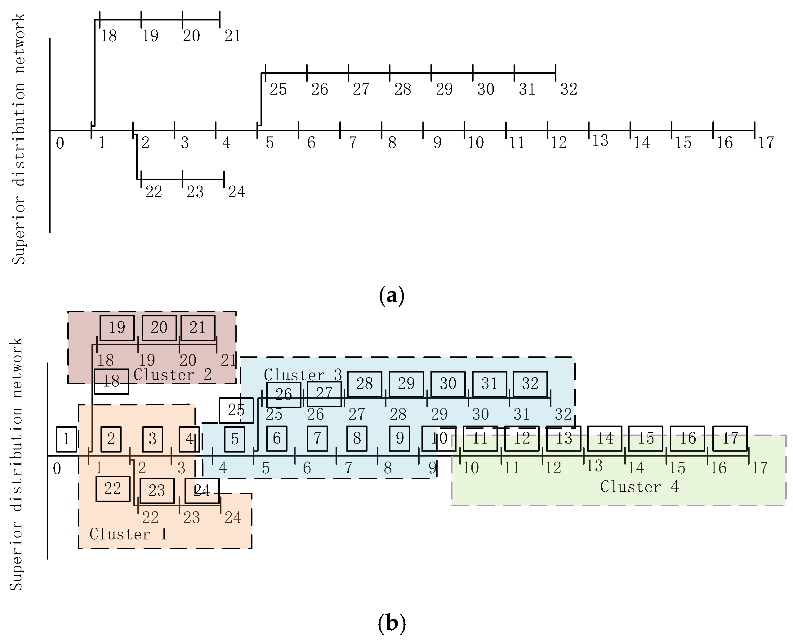
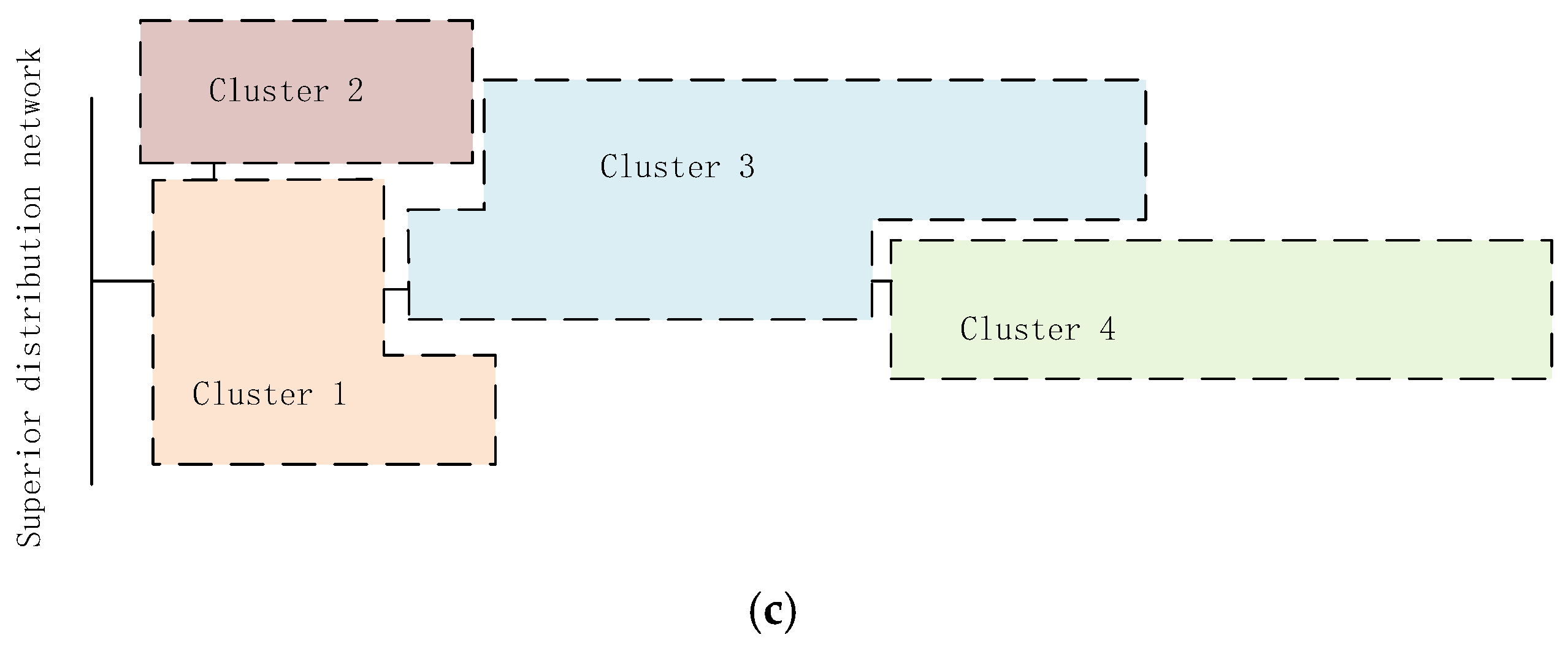
In power system analysis, the cluster partition index is a quantitative criterion used to evaluate and determine the optimal zoning scheme for distribution networks. By comprehensively considering factors such as network topological structure and electrical characteristics (such as voltage and power), it divides complex power grids into multiple relatively independent sub-clusters with strong internal connections, so as to achieve coordinated control of distributed power sources, fault isolation, and optimal scheduling. The comprehensive performance index of clusters can be constructed by integrating multiple single-item indicators related to the operation of the distribution network. It is a quantitative basis used to comprehensively evaluate the effect of cluster partitioning and operational characteristics. Using the cluster partition index proposed in Ref. [15], the power grid is divided into a several sub-clusters (or sub-regions) structure, and the best partitioning schemes are obtained by calculating the comprehensive performance index, so as to obtain the cluster partition results, as shown in Figure 1.
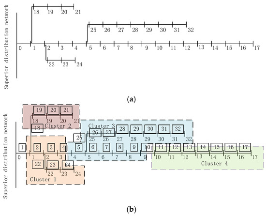
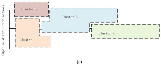
Figure 1.
Flow chart of cluster partition algorithm: (a) Former IEEE33-node distribution network structure; (b) Cluster demarcation; (c) Superstructure—clusters as the basic unit.
In the simulation, node 14 is connected to a 150 kW wind power system, while node 29 is linked to a 300 kW wind power source. Similarly, nodes 20 and 23 are connected to 100 kW and 300 kW of wind power, respectively. Detailed data for both wind and photovoltaic power are sourced from reference [20].
The following is a brief discussion of the results of this division to clarify the idea of two-level planning in this paper.
In this cluster structure, there are the following three types of branches: (1) intra-group branches, which are branches that connect nodes in the same cluster, just like branches 5–9 in Cluster 3 in Figure 1b; (2) inter-group interactive branches, connecting branches of different clusters, such as branches 4, 10, 18; (3) The main network liaison branch, the branch that connects the bus and the nodes in a certain cluster, such as branch 1 between the upper-level distribution network and Cluster 1 in Figure 1b.
2.3.2. Upper-Level Planning—With Clusters as the Basic Unit
After the cluster division is completed, the distribution network-multi-cluster layer shown in Figure 1c is constructed. In this paper, the upper-level planning with clusters as the basic operating unit takes the constructed multi-cluster distribution network as the research object, regards each cluster as an equivalent node, and co-optimizes DPV and ESS capacities, along with power connected to each cluster according to the total load of each cluster, considering the relative size and time sequence change trend of the load between the clusters.
2.3.3. Lower-Level Planning (Node-Based)
Under the premise that the total DPV and ESS capacity of each cluster are determined through upper-layer planning, the different DPV access capacity of each node in the cluster and the grid-connected location of the ESS will affect the entire power distribution system. Therefore, the lower layer takes the cluster-node layer as the research object to carry out DPV addressing, capacity distribution and ESS site selection planning in each single cluster. In particular, the lower-level planning algorithm adopts a parallel configuration method to optimize the DPV capacity of nodes in each cluster and the location layout of ESS. This method not only considers the mutual influence relationship of the optimization process of the decision variables of each cluster, but also realizes parallel computing, which effectively improves the operation efficiency and calculation accuracy.
3. DPV and ESS Siting and Capacity Bi-Level Planning Model
3.1. Two-Tier Planning Architecture
A two-layer coordinated planning model of DPV and ESS site and capacity is established according to the distribution network-cluster-node hierarchical planning strategy described in Section 2.3, and the model architecture is shown in Figure 2.
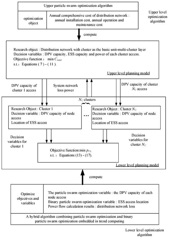
Figure 2.
Framework of planning model.
In the upper-level planning model, the planning objective is to minimize the annual comprehensive cost of the distribution network. The decision variables include the overall DPV capacity, ESS capacity, and power assigned to each cluster. Constraints include the DPV installed capacity constraint of each cluster, the switchover power constraint of the main network liaison branch, the power constraint of the inter-group alternate branch, the charging and releasing power constraint of ESS, and the state of charge constraint of ESS.
In the lower-level planning model, the planning objective is to minimize the power loss of the distribution network. The decision variables are the DPV sub-capacity at each node and ESS placement. Constraints encompass DPV capacity, distribution network power flow, node voltage, and branch power limits. A two-layer stacked hybrid particle swarm optimization method, integrated with AC power flow calculation is applied to resolve the issue.
Parameter transfer relationship between two-level programming models: the upper and lower optimization problems of the two-level programming model have their own objective functions, decision variables, and constraints, but the optimization process of the upper and lower planning is interdependent. On this basis, the lower level planning model optimizes the capacity of the DPV and ESS access location connected to each node in the cluster-node layer, calculates the tidal flow according to the optimization results, obtains the system network loss power, and feeds it back into the active power balance equation constraint of the upper-layer planning as a parameter.
3.2. Upper-Level Planning Model
Utilizing clusters as its fundamental unit, the upper-level planning model aims to determine the total DPV and ESS resources for each cluster. Its objective is minimizing the distribution network’s annual cost by planning the DPV capacity, ESS capacity, and power allocations.
3.2.1. Objective Function
In the formula, CTotal represents the total annual expense of the distribution network, including the equivalent annual installation cost of DPV and ESS (CI), the yearly O&M expense of the system (COM), the annual DPV generation subsidy (CPS), and the main network power purchase cost (CP).
- (1)
- Equal yearly installation expense.
- (2)
- Annual operation and maintenance costs.
- (3)
- DPV annual power generation subsidy.
- (4)
- The expenditure for electricity sourced from the primary network.
3.2.2. Constraints
- (1)
- The DPV capacity constraints that cluster j allows to be installed.
- (2)
- Power balance constraints.
- (3)
- Mainnet liaison branch reversing power constraint.
- (4)
- Inter-group interactive branch power constraints.
- (5)
- DPV active output constraint, i.e., the DPV output power is less than the rated capacity of the installation.
- (6)
- ESS charge–discharge power and state-of-charge constraints.
The charge–discharge power and state of charge of the ESS need to meet certain constraints:
where is the maximum output power of ESS in cluster j; ηt is the charging and discharging efficiency of ESS at time t; ηd is the discharge efficiency; ηc is the charging efficiency; Sj,t is the state of charge of the ESS in thse cluster j at time t; Smin and Smax are the minimum and maximum values of the state of charge of ESS, respectively. S0 is the initial state of charge of the ESS.
3.3. Lower-Level Planning Model
3.3.1. Objective Function
The objective function of the lower-level planning is the minimum loss of the entire distribution network, and its mathematical expression is
where pCL is the distribution network loss.
3.3.2. Constraints
The DPV capacity of each node in the cluster j is constrained by the upper-level decision variable (the total DPV capacity of each cluster).
- (1)
- The DPV capacity constraint of each node in the cluster j.
- (2)
- The DPV capacity constraints that node i allows for installation.
- (3)
- Distribution network power flow constraints.
The safe operation of the system needs to meet the node voltage constraints and branch power flow constraints.
- (4)
- Node i voltage constraints.
- (5)
- Branch l power constraint.
4. Solving Algorithm for the Two-Level Programming Model
4.1. A Two-Layer Iterative Hybrid Particle Swarm Algorithm Embedded in Power Flow Computing
This paper addresses the dual-layer planning model for site selection and capacity determination. Based on particle swarm optimization and binary particle swarm optimization algorithms, it integrates AC power flow calculation to construct a hybrid particle swarm algorithm. Specifically, the particle swarm algorithm is used to encode and solve the upper-level variables, while the particle swarm and binary particle swarm algorithms are integrated to solve the continuous space optimization and combinatorial optimization problems of the lower-level planning, respectively. The lower-level objective function values are obtained through AC power flow calculations. By exchanging information between the dual-layer particle swarms, the iterative solution of the dual-layer planning problem for distributed power source site selection and capacity determination is achieved.
The hybrid particle swarm algorithm is based on the idea of interactive iterative nesting. In each iterative optimization process, the two-layer planning passes its optimal solution as feedback information to the other layer planning, respectively. The other layer planning makes corresponding decision adjustment on this basis. In this way, the iterative interaction is repeated and the optimal solution of the two-layer planning problem is obtained finally. Among them, we define the basic iteration number variable of the particle swarm optimization algorithm as “iter”, which is used to record the number of iterations that the algorithm has carried out from the start to the current moment. We define the iteration number variable of the improved particle swarm optimization algorithm as “iteru”, which is used to represent the number of iterations in special cases. They are helpful for controlling the execution process of the algorithm and evaluating the performance of the algorithm.
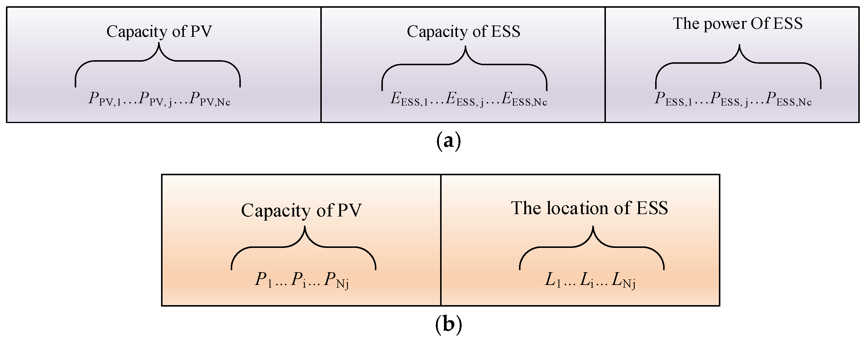
In the proposed two-layer hybrid particle swarm algorithm, the particle structures of the upper and lower layers are shown in Figure 3.
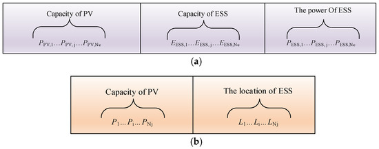
Figure 3.
Designed particle structures in both layers: (a) Upper particle encoding; (b) Underlying particle encoding.
Each particle of the superstructure consists of three parts: the DPV capacity PPV,j connected to the clusters, the ESS capacity EESS,j, and the power PESS,j as shown in Figure 3a.
Each particle of the underlying plan consists of two parts: the DPV capacity Pi connected to each node and the position Li of the ESS, as shown in Figure 3b, wherein, the DPV capacity PPV,i,j connected to each node in cluster j is full (13), and the access location of ESS in cluster j satisfies the following constraints:
where Li,j can be 0 or 1, Li,j = 0 means that node i in cluster j does not have ESS installed, and Li,j = 1 indicates that node i in cluster j is configured with ESS.
4.2. Optimize the Algorithm Process
Based on the designed particle structure for each layer, the specific steps to implement the double-layer mixed population algorithm are as follows:
- (1)
- Step 1: Initialization. Enter the distribution network’s original data to be planned, perform the initial power flow calculation, obtain the branch tidal current and node voltage data, and initialize the algorithm parameters.
- (2)
- Step 2: Initialize the upper particle swarm. Based on the value range of the upper-level programming decision variables, initialize the swarm’s velocity, position, individual optimal value, and population optimal value; set the current iteration count to iteru = 0.
- (3)
- Step 3: The upper-layer particle swarm is updated. Update the velocity and position of the upper-layer particles, and determine if the updated value satisfies the condition: if the velocities before and after the update are the same, multiply the current velocity by a random number between (0,1); if the updated position is out of bounds, the out-of-bounds particles are processed by using the boundary variation strategy of spatial scaling and attractor [22], and the number of iterations iteru is updated to iteru + 1.
- (4)
- Step 4: Lower Optimization. Follow these steps:
- Initialize the underlying particle swarm. Based on the upper particles, initialize the velocity and position of the lower particles for each cluster, set the individual and group optimal values, and set the iteration count (iter) to 0.
- Update the lower particle swarm. Update the particles for DPV capacity at each node in the lower layer (step 3) and optimize the ESS position using the binary particle swarm formula. Increment the iteration count (iter) by 1.
- Evaluate the fitness of the lower particles. Using the lower-layer particle data, update the DPV output and ESS charge/discharge power at each node in the power flow program, then perform power flow calculations to determine the fitness of the lower subgroups.
- Update the individual and population optimal values and fitness of the lower particle swarm. The swarm’s fitness was compared with the corresponding individual optimal fitness, and the optimal values and fitness were updated. Moreover, the individual optimal value and individual optimal fitness were updated. Then, the individual optimal fitness was compared with the current population optimal fitness, and the population optimal value and group optimal fitness were updated.
- Judgment on the number of iterations. Determine whether the condition iter < max iter (max iter = max iteru/10) is satisfied, and if so, return 2); otherwise, the current population optimal value and fitness are used as optimization results, and step 5 is turned.
- (5)
- Step 5: Calculate the fitness of the upper particles. Based on the current population particle data, the particle fitness is obtained.
- (6)
- Step 6: Update the individual and population optimal values and fitness of the upper particle swarm. Same as step 4.
- (7)
- Step 7: The number of iterations is checked. If the condition iteru < max iteru is met, return to step 3; otherwise, output the results of double-layer sitting and capacity optimization.
The detailed process of the two-layer hybrid particle swarm optimization in the power flow calculation is shown in Figure A1.
4.3. Operational Performance Evaluation Index
In this section, the evaluation indicators of DPV and ESS configuration are proposed from four aspects: improved self-balancing [23], energy permeability, capacity permeability, and power permeability [24].
- (1)
- Improved self-balancing degree SA,j:
In the formula, SCl,j is the number of inter-group interaction branches connected to cluster j. The self-balancing degree SA,j index reflects the annual overall support of the DPV-ESS output to the load in the cluster and the autonomy of the cluster.
- (2)
- Energy permeability SEP: the ratio of the annual output of the DPV in the cluster to the annual power demand of the load in the cluster, reflecting the cumulative effect of the DPV output to the load.
- (3)
- Capacity permeability SCP: the ratio of the annual maximum DPV output to the annual maximum load in the cluster, reflecting the saturation degree of DPV capacity and its limit.
- (4)
- Power permeability SPP: the annual maximum ratio of DPV output to load. It reflects the maximum proportion of load electricity demand that DPV power can meet within a cluster during a specific planning period and demonstrates the upper limit of the supporting capacity of distributed PV power sources for local loads.
5. System Examples and Result Analysis
5.1. Simulation Verification of a Typical IEEE33 Node System
In order to further verify the applicability and effectiveness of the proposed two-layer optimization model in large-scale power distribution systems, this paper selects the latest typical IEEE33-node power distribution system as an example for extended simulation analysis; Figure 4 shows the network structure of the IEEE33 node system. The system consists of 33 nodes and 32 branches, the backbone line is a tree-like structure, the system voltage level is 12.66 kV, and the base load data and network topology are from the standard IEEE test system. In order to fit the practical application scenarios, this paper makes appropriate adjustments to the original load data and introduces the typical daily load curves of photovoltaic output and energy storage systems.

Figure 4.
IEEE33 node system network diagram.
5.1.1. The Clustering Results of the Typical IEEE33 Bus System
According to the distribution network cluster division method based on electrical coupling degree and power balance degree proposed in this paper, the IEEE33 node system is divided into clusters. The electrical similarity between nodes was calculated by using the node voltage sensitivity analysis method and the power flow distribution weight coefficient, and the system was divided into four clusters by combining the spectral clustering algorithm. Figure 5 shows the distribution of nodes in the topology diagram and the corresponding cluster numbers.
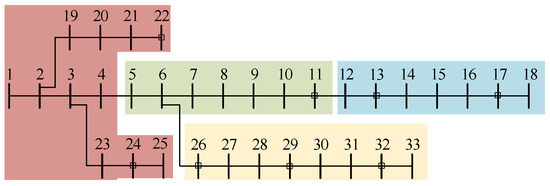
Figure 5.
IEEE33 node system cluster partition results.
5.1.2. Optimize the Configuration Result
Based on the divided cluster structure, a two-layer optimization model was constructed for simulation analysis. Consider the following three configuration scenarios:
Option 1: Configure only distributed photovoltaic (DPV);
Option 2: Configure only the energy storage system (ESS);
Option 3: Configure the synergy scheme between DPV and ESS (proposed two-layer model).
The optimization goal is to minimize the comprehensive operating cost of the system, including power purchase costs, energy storage operating costs, and network loss costs. Table 1 shows a comparison of the optimization results of the three schemes.

Table 1.
Costs under different scenarios.
As can be seen from the table, Option 3 is the best in terms of system comprehensive cost, which verifies the effectiveness of the proposed collaborative configuration method in large-scale systems.
5.1.3. Sensitivity Analysis
In order to further verify the robustness of the model, two key parameters are analyzed for sensitivity.
- (1)
- The impact of PV permeability changes on system costs
The PV penetration rates were set to be 20%, 40%, 60%, and 80%, respectively, and the changes in the comprehensive cost under each scenario were compared, as shown in the table. The results show that with the increase in photovoltaic penetration, the system power purchase cost continues to decrease, but when the penetration rate exceeds 60%, the system network loss and energy storage cost increase slightly due to the increase in power return transmission problem (Table 2).
Table 2.
The impact of PV permeability changes on system costs.
With the PV penetration rate increasing from 20% to 80%, the system power purchase cost has gradually decreased from about $11,137.16 to about $9098.49. This reflects the increase in photovoltaic power generation, which significantly reduces the need to purchase electricity from the grid. At a low penetration rate (20–40%), the cost of grid loss increased from about $696.71 to about $764.33, and the cost of energy storage increased from about $423.35 to about $444.65, with a relatively flat increase. However, when the penetration rate reaches 60–80%, the cost of grid loss rises from about $835.71 to about $976.26, and the cost of energy storage rises from about $488.21 to about $560.80 due to the aggravation of the power return problem (PV output exceeds the local load, resulting in power retransmission to the upper power grid), showing a more obvious irregular growth. The combined cost reached its lowest value of about $11,091.98 at 60% PV penetration, and then rose slightly to about $10,635.55 at 80%. This shows that a moderate PV penetration rate (40–60%) can effectively reduce the system cost, but an excessively high penetration rate (80%) will partially offset the economic benefits due to the increase in grid loss and energy storage costs, reflecting the balance between system operation constraints and costs.
- (2)
- The impact of changes in electricity price levels on optimal allocation
The fluctuation coefficients of electricity prices are set to ±10% and ±20%, respectively, and the optimal configuration is re-solved, and the results are shown in Table 3.
Table 3.
The impact of the change in electricity price level on the configuration capacity of the energy storage system.
When the fluctuation coefficient of electricity price is −20%, the electricity price is significantly lower than the benchmark level, the purchase cost of electricity is lower, and the economics of the energy storage system are weakened, so the configured capacity is only 1023.45 kWh. With the gradual recovery of electricity prices to −10%, the configured capacity increased to 1198.76 kWh, showing a steady growth.
When the fluctuation coefficient of electricity price is +10% and +20%, the electricity price is 10% and 20% higher than the benchmark level, respectively, and the energy storage system can significantly reduce the power purchase cost through peak shaving and valley filling in the environment of high electricity price, so the configured capacity increases to 1789.01 kWh and 2034.56 kWh, respectively, which is more obvious.
There is a positive correlation between the allocation capacity of the energy storage system and the electricity price level. When the electricity price is low, the economy of energy storage is not significant, and the configuration capacity is small. When electricity prices are high, energy storage can optimize operating costs and significantly increase the allocated capacity. Slight irregularities in the data (e.g., increments fluctuating between 200 and 300 kWh) reflect possible system constraints or computational accuracy during the actual optimization process.
Through the extended simulation analysis of the IEEE33 node system, the adaptability and effectiveness of the proposed two-layer optimal configuration model in different scale distribution systems are further verified. The simulation results show that the co-configuration of DPV and ESS can significantly reduce the comprehensive cost of the system, improve the voltage stability, and have good economic and engineering feasibility. At the same time, the sensitivity analysis shows that the model has good robustness in the face of parameter fluctuations, which provides theoretical support for subsequent practical engineering applications.
5.2. Overview of Actual System Examples
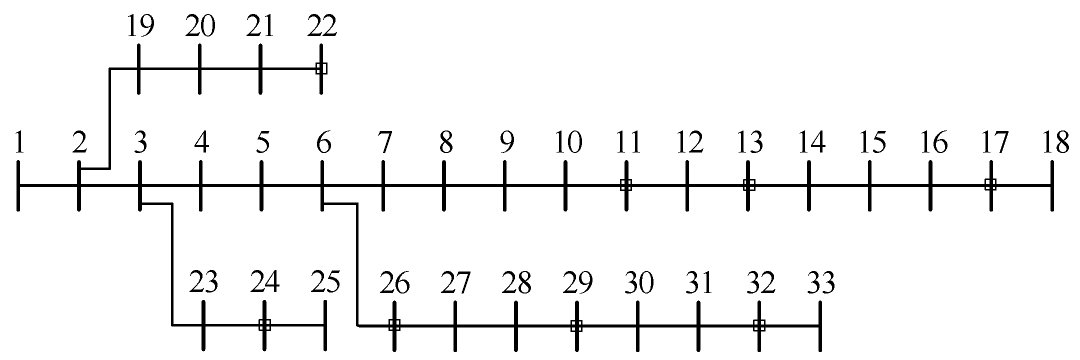
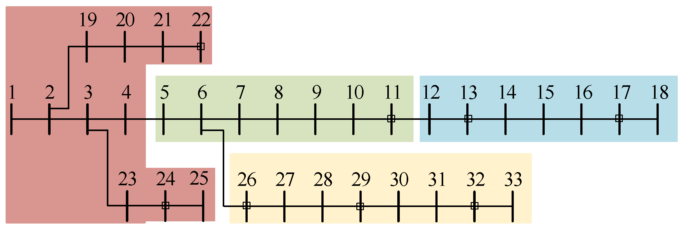
In order to further verify the accuracy of the model, this paper uses the 10 kV distribution system of a “regional decentralized” DPV power generation poverty alleviation demonstration area as an example for simulation analysis. The distribution line topology is shown in Figure 6a, and Figure 6b is the result of cluster partitioning.
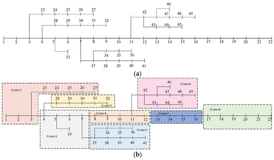
Figure 6.
Distribution system cluster structure of the planning area: (a) the distribution network structure of the original planning area; (b) the result of multi-cluster division in the planning area.
The grid structure of this example includes 49 nodes, of which 29 are load nodes, and the total active load annual maximum is 1169.6 kW. The output from the DPV and the power data from the load are derived from measurements taken in the region in 2016. These data form the basis for the analysis presented, in which there are two peak daily consumption periods, 8:00–10:00 and 18:00–21:00, which are typical residential loads. The annual solar irradiance (standard unit value) curve for this region is referenced [14].
First, the cluster-division indices mentioned earlier are adopted to divide the power grid into several sub-cluster structures. By calculating the comprehensive performance indices, the optimal number of partitions and partition boundaries are obtained, thus achieving the cluster-partitioning results. After the cluster division is completed, a bi-level programming model is utilized. At the upper level, with clusters as basic units, the distribution network-multi-cluster layer is constructed. The upper level consists of the main distribution network, main-network tie-lines, equivalent nodes of each cluster, and inter-cluster interaction branches. Given that the total capacities of distributed photovoltaic (DPV) and energy storage systems (ESS) in each cluster are determined through the upper-level planning, different access capacities of DPV at each node within the cluster and grid-connection locations of ESS will affect the power losses of the cluster and the entire distribution system. At the lower level, taking the cluster-node layer as the research object, the siting and sizing of DPV and siting planning of ESS within each single cluster are carried out.
The simulation analysis of sodium sulfur battery (NaS) is carried out as an example. The technical and economic parameters of DPV and NaS are shown in Table A1. The system achieves optimal economic performance when the ratio of the rated power to the rated capacity of NaS is set to 1/3. For the particle swarm optimization simulation, the following parameters are specified: a population size of 20,500 upper-level iterations, a maximum inertia weight coefficient of 0.9, and a minimum inertia weight factor of 0.4.
5.3. Case Results and Case Comparison Analysis
5.3.1. DPV and ESS Site Selection and Capacity Planning Scheme
To emphasize the benefits of the proposed hierarchical planning approach, this paper develops three distinct planning scenarios. These are used to compare and analyze the challenges of determining the optimal locations and capacities for DPV and ESS in the distribution network under various conditions.
To clarify that all scenarios (the original system, Scheme 1, Scheme 2, and Scheme 3) are based on the same 10 kV distribution network structure, load data, illumination data, and ESS technical parameters (NaS battery, the parameters are shown in Table A1), we have controlled the variables of the network topology, load and photovoltaic data, and the parameters of the optimization algorithm:
For the network topology, all schemes adopt the original network structure in Figure 6a, and only Scheme 2 and Scheme 3 are based on the same clustering division results (Figure 6b). In terms of the load and photovoltaic data, all scenarios use the measured load curve in 2016 and the same photovoltaic output model (refer to [14,20]). In the parameter design of the optimization algorithm, the population size (20), the number of iterations (500 times for the upper layer), and the inertia weight (0.4–0.9) of the Particle Swarm Optimization (PSO) algorithm are kept consistent in all schemes. The requirement for variable differences is to only adjust the configuration strategies of DPV/ESS (for example, there is no clustering in Scheme 1 and no ESS in Scheme 2), and other variables (such as electricity prices, subsidies, and network constraints) are fixed.
Scenario 1: The distribution network is not clustered. The single-layer planning model is adopted, with the node as the basic unit, the DPV capacity, ESS capacity, and power connected to each node are directly planned, and the candidate installation nodes of the ESS are determined to be 3, 6, 8, 12, 14, 16, 21, 22, 25, 26, 30, 40, and 47 according to the time voltage sensitivity index [4], and the number of ESS that can be accessed is 8.
Scenario 2: No ESS scenario. Based on the results of cluster division, a two-layer planning model is adopted, the upper model takes the cluster as the basic unit to plan the total DPV capacity connected to each cluster, and the lower model takes the node as the basic unit to optimize the DPV sub-capacity of each node in the cluster.
Scheme 3: Building on the outcomes of the cluster division, a two-tier planning model is implemented. The upper-tier model uses clusters as the fundamental unit to determine the total DPV capacity, ESS capacity, and the power allocated to each cluster. In contrast, the lower-tier model focuses on individual nodes within the cluster, optimizing the DPV sub-capacity and selecting the optimal locations for ESS integration at each node.
5.3.2. Upper-Level Planning Results
Figure 7 shows the DPV and ESS capacity of each cluster under different scenarios, and Table 4 shows the corresponding planning costs for each solution.
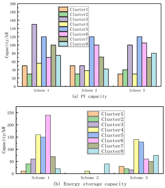
Figure 7.
DPV-ESS cluster capacity allocation results of the upper-layer planning: (a) Photovoltaic capacity; (b) Energy storage capacity.
Table 4.
Detailed costs of the upper-layer planning.
From the economic indicators shown in Table 4, it is evident that, prior to the planning, the distribution network’s load demand is entirely met through purchases from the main network. This results in a high reliance on the main network and tie lines, leading to substantial costs associated with purchasing electricity from the main network. This highlights the necessity of implementing a capacity planning strategy for the distribution network. After the planning, the electricity procurement cost from the main network across the three options has decreased. However, this cost still constitutes a significant portion compared to other expenses. The primary reasons for this are as follows: firstly, there is a temporal mismatch between the output of the DPV and the load demand; secondly, the current configuration of ESS remains costly, and its ability to shift power across different time periods is limited, which contributes to a low penetration of DPV in the distribution network.
Compare Options 1 and 3 to analyze the impact of cluster partitioning on capacity planning. As shown in Figure 7, there are significant differences between the DPV and ESS configured in Scheme 1 and Scheme 3: (1) the total capacity of the DPV connected to the distribution network in Scheme 3 is 1.26 times that of Scheme 1; (2) there are differences in the distribution of DPV capacity in each cluster in Scheme 1 and 3, the DPV in Scheme 1 is concentrated in cluster 3, while the DPV distribution among clusters in Scheme 3 is more uniform. (3) Scheme 1 has more ESS; (4) there are also some differences in the distribution of ESS among clusters under the two schemes, with the ESS mainly concentrated in clusters 4 and 6 in Scheme 1 and the more evenly distributed ESS among clusters in Scheme 3. As shown in Table 4, the main power purchase cost of Option 3 is lower, which is 135,600 yuan less than that of Option 1, but the installation cost and O&M cost are higher because of the high penetration rate of DPV in Option 3. Overall, the capacity planning approach based on cluster division enhances the total DPV capacity within the access distribution network. This strategy improves the distribution of DPV across clusters, which in turn reduces the ESS capacity required and optimizes the economic performance.
As can be seen from Figure 7, there are major differences in the DPVs configured in Schemes 2 and 3: (1) the total capacity of the distribution network in Scheme 3 is 1.29 times that of Scheme 2; (2) there are differences in the distribution of DPV capacity among clusters in Scenarios 2 and 3: the DPV in Scenario 2 is concentrated in clusters 5 and 6. As shown in Table 4, the installation cost and operation and maintenance cost of Scheme 2 are low, which are 62.76% and 76.19% of Scheme 3, respectively, and it can be seen that the installation cost ratio of Scheme 2 and Scheme 3 is lower than that of operation and maintenance cost, because Scheme 2 is not equipped with ESS, and the installed cost of ESS is higher and the operation and maintenance cost is lower, but the DPV output is intermittent and does not fully match the load in the timing, so the DPV penetration rate of Scheme 2 is low, and its DPV output is only 77.36% of Scheme 3. When the DPV output is insufficient to meet the load demand, electricity must be purchased from the main network, which increases the strain on both the main network and the tie lines. In general, integrating ESS enhances the capacity of DPVs within the distribution network, thereby reducing the reliance on electricity purchases from the main grid.
5.3.3. Lower-Level Planning Results
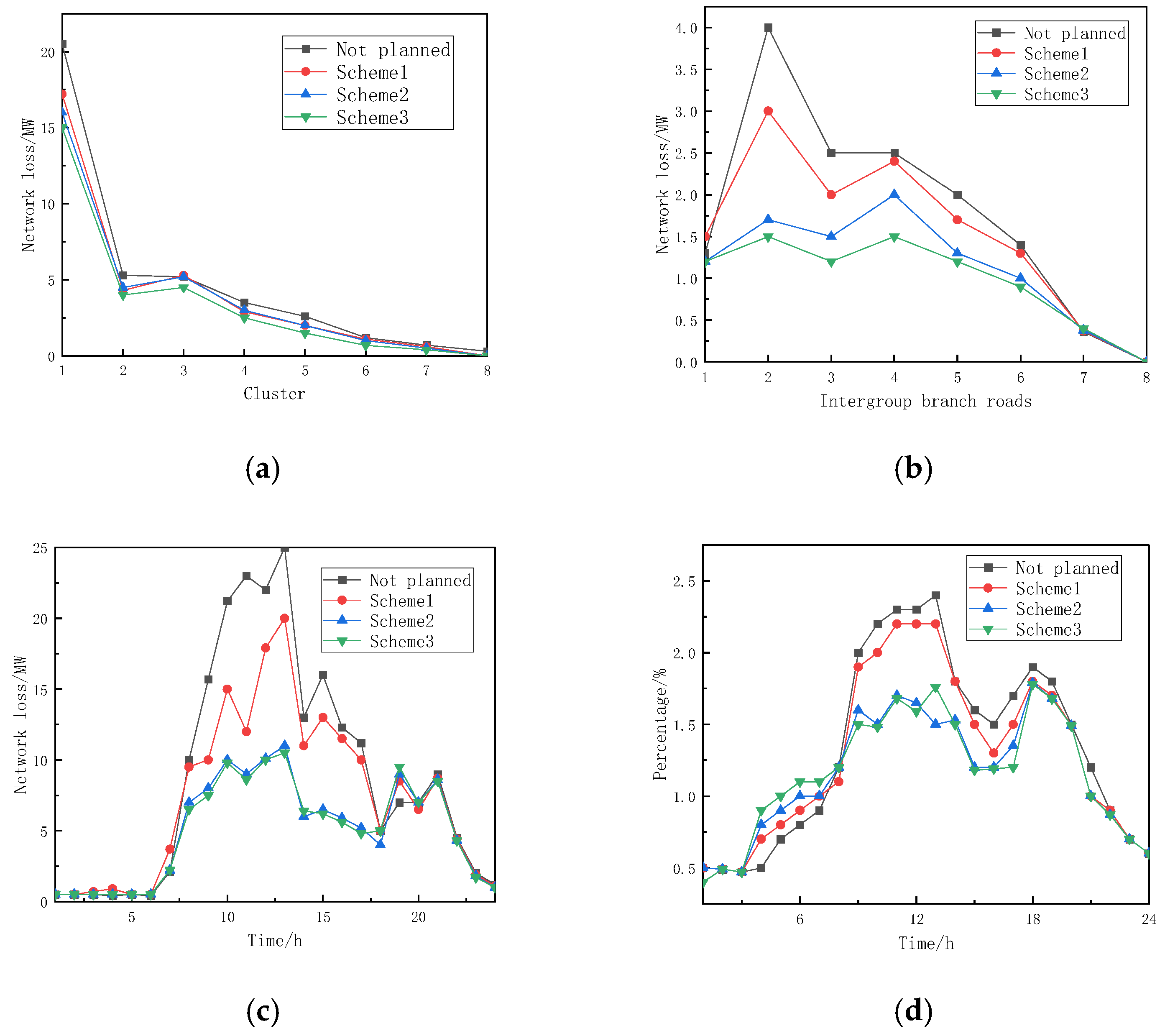
Figure 8 shows the network loss data of each scenario.
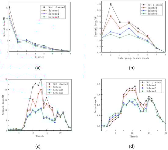
Figure 8.
Loss of the lower-layer planning under four schemes: (a) Annual network loss within each cluster; (b) Inter-group annual network loss; (c) System network loss; (d) Percentage of power loss.
Figure 8a,b show that the annual intra-group network loss and inter-group tributary network loss of each cluster in Scheme 2 and 3 are significantly lower than those of the original system and Scheme 1, among which the annual intra-group network loss of clusters 1–3 in Scheme 3 is 63.03%, 69.05%, and 71.67% of the original system, respectively, and the inter-group branch network loss is reduced to 47.59~63.65% of the original system.
It can be seen from Figure 8c,d that at 7:00–18:00, the hourly data of system network loss and the hourly data of power loss ratio (the percentage of power loss of distribution network at time t to the total power supply of distribution network) in typical days of Scheme 2 and Scheme 3 are significantly lower than those of the original system and Scheme 1. Since the DPV output meets the load demand locally during this period, the power flow through the branch is decreased, leading to a reduction in system network losses. Specifically, at 13:00, the proportion of both system network losses and power losses saw the most significant decrease, and the share of network losses in the system and power losses in Scheme 3 decreased to 37.06% and 72.69% of the original system, respectively.
In summary, the network loss of solutions 2 and 3 is markedly better than the original system, so the cluster-based DPV and ESS configuration mode significantly reduces the system’s network loss.
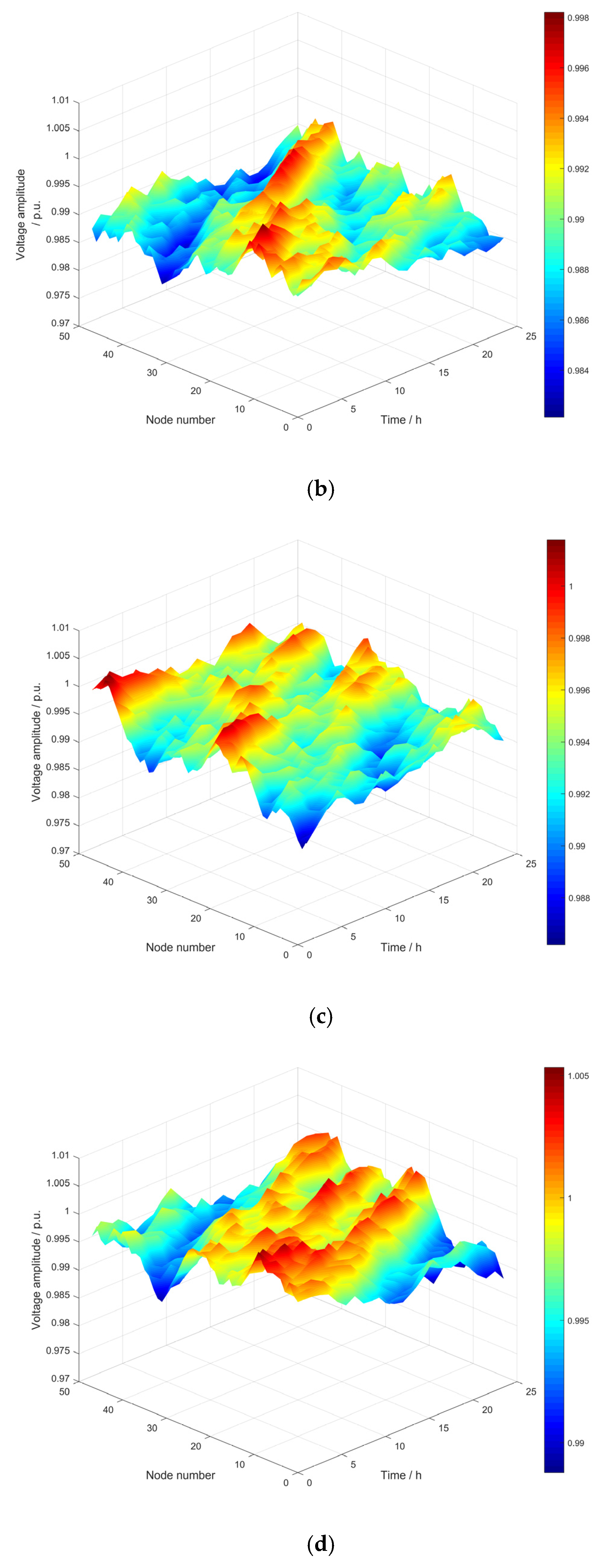
Figure 9 shows the typical daily node voltage data for each scenario. The system node voltages in pre-planning and Scheme 1 are low, with minimum values of 0.977 and 0.981, respectively, and Scheme 2 and Scheme 3 increase them to 0.985. The voltage fluctuation index [17] of the system nodes in Scheme 2 and 3 is reduced by 24.95% and 13.67% before planning, respectively. Therefore, the configuration of DPV in the system can improve the minimum value of the node voltage of the system.
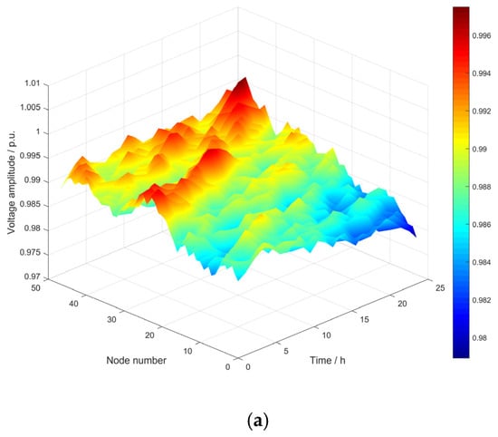

Figure 9.
Voltage curves of 49 nodes under four schemes: (a) Not planned; (b) Programme 1; (c) Programme 2; (d) Programme 3.
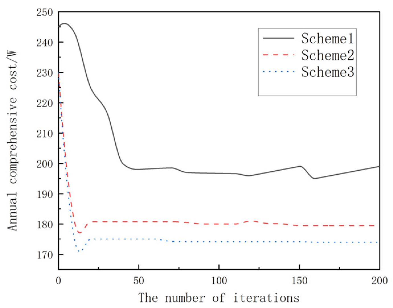
The iterative process for each scenario is shown in Figure 10. As can be seen from the graph, Options 2 and 3 can quickly converge to near the optimal value in fewer iterations, while Option 1 needs more iterations to converge to near the most efficient solution. The reason for this phenomenon is that the decision variable dimension of Scheme 1 is high, the optimization complexity is large, and the optimization process is slow. From the analysis, it can be inferred that the proposed hierarchical configuration method based on cluster division can substantially decrease the computational complexity and improve the computational efficiency while improving the economic efficiency of the distribution network.
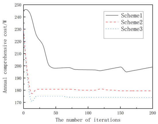
Figure 10.
Voltage curves of 49 nodes under four schemes.
5.4. Analysis of Planning Performance Evaluation Indicators
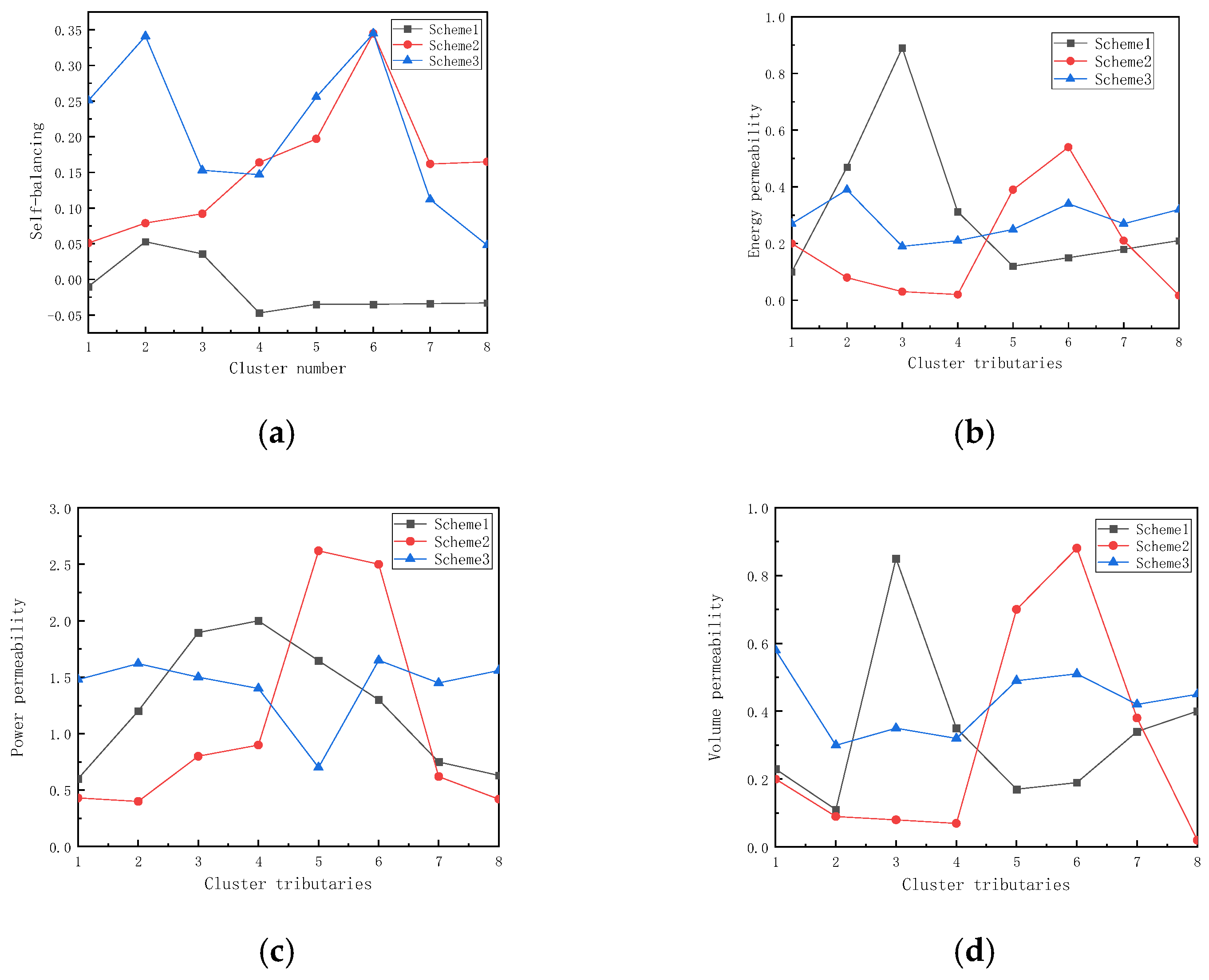
Figure 11 shows the evaluation of the indicators of each cluster under the four scenarios.
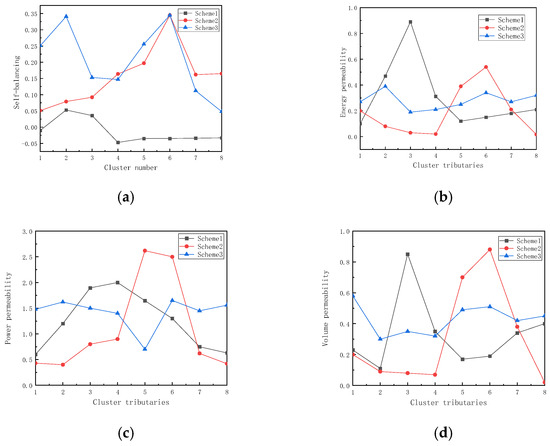
Figure 11.
Comparison of varies indices of each cluster under 4 schemes: (a) Self-balancing; (b) Energy permeability; (c) Capacity permeability; (d) Power permeability.
The closer the self-balancing degree of the cluster is to 1, the stronger the autonomous ability of the cluster is. On the contrary, the more deviated from 1, the weaker the autonomy of the cluster. From Figure 11a, it is evident that the self-balancing degree of each cluster in Scheme 3 is relatively high, stable between 0.15 and 0.35, and the distribution between clusters is relatively uniform. The reason is that the scheme is based on the cluster configuration DPV and ESS, taking into account the load timing correlation and complementarity between nodes in the group. The cluster 3 of Scheme 1 and the cluster 5 and 6 of Scheme 2 have higher self-balancing degree, while the self-balancing degree of other clusters is relatively low, and the distribution difference between clusters is large.
The penetration metric of the cluster is related to the DPV capacity of the access within the cluster. As can be seen from Figure 11b–d, cluster 3 in Option 1 has a high DPV permeability, while the other clusters have a low permeability. In Scheme 2, the DPV penetration rate of clusters 5 and 6 is high, while the penetration rate of other clusters is low, because ESS is not configured in this scheme, and the load peak of some clusters is not related to the timing of the peak output of DPV, which makes it difficult for the DPV output to meet the load demand in terms of timing, resulting in a small DPV capacity connected to the cluster. In Scheme 3, the DPV penetration rate is relatively high and the distribution among the clusters is relatively uniform, because the scheme uses the cluster as the basic unit to configure the ESS, which effectively alleviates the timing mismatch between the DPV output and the load demand and improves the DPV capacity of the clusters. The critical value of DPV capacity permeability is 1, and when the critical value is exceeded, the maximum value of DPV output in the cluster is higher than the maximum value of the load in the group, and there must be a situation where the excess output of DPV interacts between clusters. As can be seen from Figure 11c, the capacity penetration rate of each cluster does not exceed 1 under different configuration scenarios, indicating that the configuration result is more reasonable. The DPV capacity permeability, energy permeability and power permeability of the cluster were nonlinearly positively correlated.
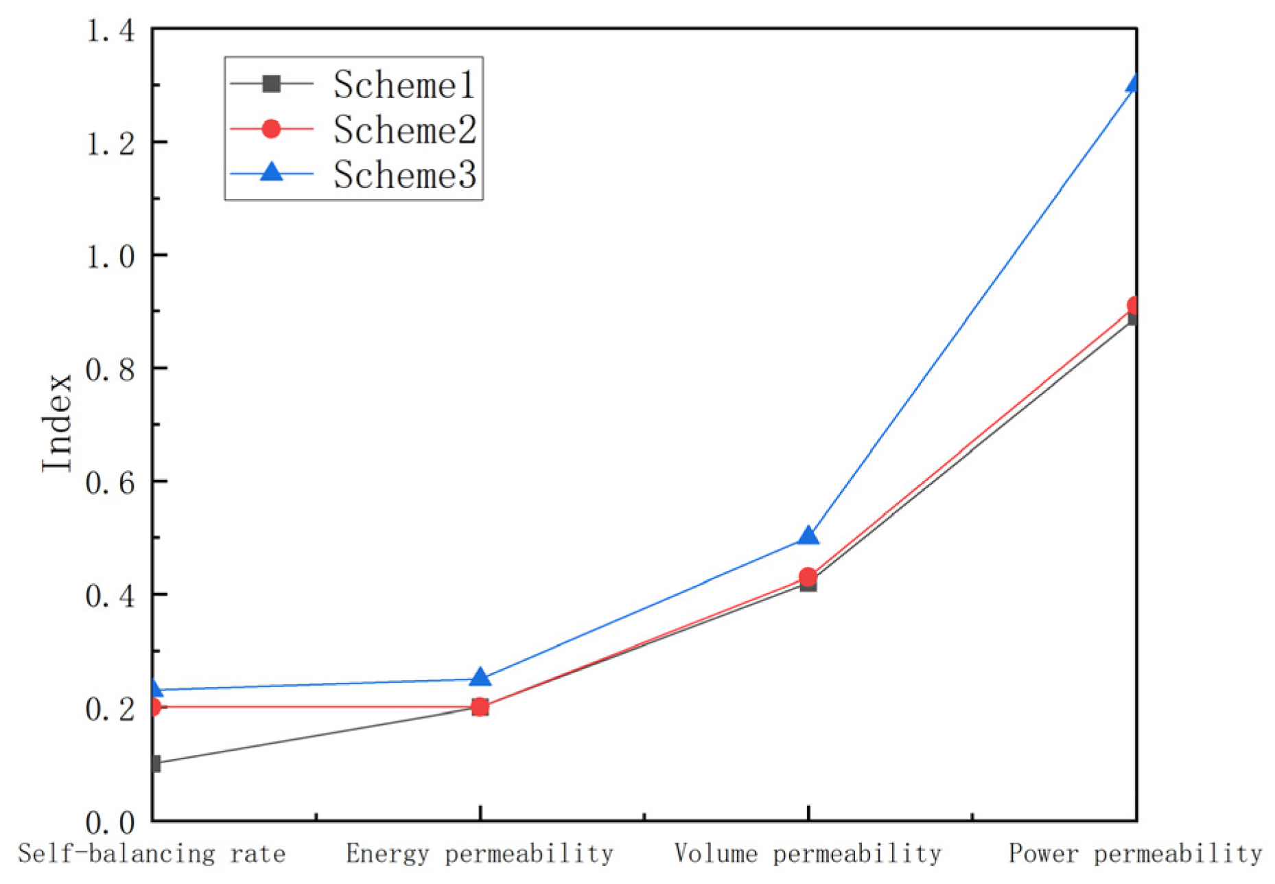
Figure 12 shows the comparison of the evaluation indicators of the distribution network under the three schemes. The diagram analysis leads to the following conclusions: (1) all the indicators of the distribution network in Scheme 3 are optimal; (2) Comparing Options 1 and 2 with Option 3, it can be seen that cluster-based DPV and ESS capacity planning improves the penetration of DPV in the distribution network and the autonomy of the system.
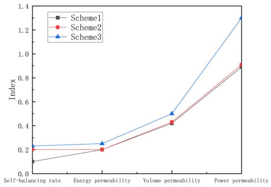
Figure 12.
Comparison of various indices of distribution network under three schemes.
5.5. Analysis of the Impact of ESS Type on Planning Results
In this paper, sodium-sulfur batteries (NaS), vanadium redox batteries (VRBs), polysulfide bromine batteries (PSBs), value-regulated lead-acid batteries (VRLA), and lithium-ion batteries (Li-ion) were selected. For each type of ESS, the proposed planning model and method based on cluster division were used to plan the DPV and ESS of the above-mentioned 10 kV feeder system, and the optimization results were compared and analyzed, and the relevant parameters of each type of ESS are referred to [25]; see Table A2 in Appendix A for details. The planning costs, network loss data, and DPV and ESS capacity optimization results of different types of ESS are presented in Table 5, Table 6 and Table A3, respectively.
Table 5.
The planning cost corresponding to different types of ESS.
Table 6.
Loss of each type of ESS.
From Table 5 and Table 6 and Appendix A Table A3, the scheme corresponding to PSB has the best economy, the lowest system network loss, and the highest DPV penetration rate of the access system in this scheme. The second solution is VRB, followed by NaS, VRLA, and Li-ion, and the economic indicators, system network loss, and capacity configuration results of the three types of ESS are relatively similar.
The impact of different types of ESS on optimization results and planning performance is mainly caused by the differences in unit investment cost, charge–discharge efficiency, and service life of ESS [26]. Among them, VRLA and Li-ion have the highest charging and discharging efficiency, but VRLA’s short service life makes it the highest annual investment cost of Li-ion, so its economy is lower. Although the charging and discharging efficiency of PSB is slightly lower, its unit capacity and power investment cost are much lower than the other four types of ESS, and the economy is more prominent, and the main reason that restricts ESS access to the distribution network at present is that the investment cost of ESS is too high, so the ESS capacity and power of PSB corresponding scheme access to the distribution network are the highest, thereby improving the access capacity of DPV, and then reducing the annual comprehensive cost and system loss of distribution network. VRBs have a higher investment cost per unit of power and a lower investment cost per unit capacity, resulting in the lowest power/capacity ratio for ESS connected to the distribution network. Hence, in the implementation of DPV cluster planning for distribution networks, using ESS technologies such as PSB or VRB can be advantageous. These options not only enhance the penetration of DPV within the distribution network but also improve the economic efficiency of the planning process while simultaneously reducing the system’s network losses.
Building on the analysis above, this section simulates the distribution network planning for different types of ESS, and the results show that the planning model and approach reliant on cluster division suggested in this study are suitable for many types of ESS.
5.6. Analysis of Algorithm Performance
In order to fully demonstrate the superiority and scalability of the Hybrid Particle Swarm Optimization (HPSO) algorithm proposed in this paper, a comparative experiment is designed. The performance of HPSO is compared with the Genetic Algorithm (GA), the classical nonlinear optimization algorithm (represented by the Sequential Quadratic Programming method, SQP), and the Reinforcement Learning algorithm based on neural networks (DRL). The IEEE 33-node distribution network system is selected as the test object to evaluate the performance of the algorithm for problems of different scales. All the comparative algorithms are adjusted to the optimal parameter configuration through multiple pre-experiments to ensure a fair comparison. For example, the crossover probability of the Genetic Algorithm is set to 0.8, the mutation probability is set to 0.02; the learning rate of the Reinforcement Learning algorithm is set to 0.001, and the size of the experience replay buffer is set to 10,000.
The specific contents include the comparison of time and solution quality. Among them, the solution quality takes the annual comprehensive cost (USD) as the core indicator for measuring the solution quality, and a lower value indicates a better solution. The comparison of calculation time and solution quality is shown in Table 7.
Table 7.
Comparison Table of Calculation Time and Solution Quality for the 33-node System.
As can be seen from the data in the table for the 33-node distribution network system, the calculation time of the Hybrid Particle Swarm Optimization (HPSO) algorithm is significantly shorter than that of other comparative algorithms. The calculation time of HPSO is only about 42.3% of that of the Genetic Algorithm (GA), 55.8% of that of the Sequential Quadratic Programming (SQP) algorithm, and 33.3% of that of the Reinforcement Learning algorithm (DRL). This clearly demonstrates the high efficiency of the HPSO in calculation.
In terms of solution quality, taking the annual comprehensive cost as the core indicator for measuring solution quality, the annual comprehensive cost obtained by the HPSO is 185.7, which is lower than the 202.1 of the GA, the 193.4 of the SQP, and the 208.6 of the DRL. This indicates that the HPSO can find a more optimal planning scheme for distributed power sources and energy storage systems in the 33-node system, effectively reducing the operation cost of the distribution network and reflecting its superiority in obtaining high-quality solutions. It shows that the HPSO has obvious advantages in both calculation efficiency and solution quality for the 33-node system.
Through the above comparative experiments and data analysis, the significant advantages of the Hybrid Particle Swarm Optimization (HPSO) algorithm over other competing algorithms in terms of calculation efficiency and solution quality as well as its good scalability in distribution network planning problems of different scales are clearly demonstrated.
6. Conclusions
6.1. Research Work Summary
This study considers the interaction between planning and operational optimization problems at various time scales. Building upon the division of the distribution network into clusters, a two-layer coordinated location and capacity planning model for DPV and ESS is developed. To solve this problem, a two-layer iterative hybrid particle swarm optimization algorithm, integrated with power flow calculations, is employed. Using a real-world distribution network system as a case study, the simulation results demonstrate that
- (1)
- The proposed approach configures the ESS based on clusters, effectively addressing the timing mismatch between DPV output and load demand. In the case study of the 10 kV distribution system, compared with Scenario 1 (non-clustered single-layer planning model), the total DPV capacity connected to the distribution network in Scenario 3 (cluster-based two-layer planning model) increased by 26%. Meanwhile, the cost of purchasing electricity from the main network decreased by 135,600 yuan. This indicates that the approach enhances the distribution network’s capacity to integrate DPV by 26%, reduces the strain on the main network and tie lines, and ultimately improves the economic performance of the distribution network’s operation.
- (2)
- The proposed method incorporates zoning during the planning phase, which brings significant improvements. In Scenario 3, compared with the original system, the annual intra-group network losses of clusters 1–3 decreased to 63.03%, 69.05%, and 71.67% of the original system, respectively, and the inter-group branch network losses decreased to 47.59–63.65% of the original system. During 7:00–18:00 of a typical day, the proportion of system network losses and power losses in Scenario 3 decreased significantly. At 13:00, the proportion of system network losses decreased to 37.06% of the original system, and the proportion of power losses decreased to 72.69% of the original system. Also, the minimum node voltage increased from 0.977 before planning to 0.985 in Scenario 3, and the voltage fluctuation index decreased by 13.67% compared with that before planning. Additionally, the hierarchical planning in Scenario 3 converges faster with fewer iterations, greatly boosting the optimization efficiency.
- (3)
- The configuration results of each scheme are compared from the two levels of distribution network and cluster using comprehensive indicators. At the cluster level, in terms of the self-balancing indicator, the self-balancing degree of each cluster in Scenario 3 is relatively high, ranging stably between 0.15 and 0.35, and it is evenly distributed among clusters. In contrast, in Scenario 1, only cluster 3, and in Scenario 2, only clusters 5 and 6 have relatively high self-balancing degrees, while others are low with large distribution differences. For the Energy permeability, Capacity permeability, and Power permeability indicators, the DPV penetration rate in Scenario 3 is relatively high and evenly distributed among clusters. For example, in the Capacity permeability indicator, the values of each cluster in Scenario 3 do not exceed the critical value of 1, indicating a more reasonable configuration. At the distribution network level, Scenario 3 shows the best performance in indicators such as self-balancing rate, energy permeability, capacity permeability, and power permeability. The comparison results verify that the proposed cluster-based planning method can effectively improve the autonomy of the cluster and distribution system.
Based on considering the operation performance of the distribution network, it is necessary to establish a cluster division and distributed power planning model that comprehensively considers the uncertain factors, and at the same time consider the correlation between the cluster division problem and the optimal layout of distributed power generation, and then seek an efficient calculation method, which is a problem that needs further research.
6.2. Outlook for Follow-Up Work
Limited by the research cycle and the author’s academic ability, this paper only studies the optimal planning of distributed generation clusters in a deterministic environment, and there is still room for improvement in the constructed planning model and solution algorithm. Based on the existing research foundation, in-depth exploration will be carried out on the planning of distributed generation clusters considering uncertainty factors in the future. The specific research directions are as follows:
- (1)
- In view of the various uncertainty factors in the division of distributed generation clusters and the planning of distributed power sources, it is necessary to use the uncertainty theory to systematically analyze their influence on the complexity of distribution network operation and control and the planning results, and it is important to deeply improve the index system and division method of cluster division, as well as the optimization model and solution algorithm of power source planning.
- (2)
- In the uncertainty scenario, there is a strong coupling relationship between the division of distributed generation clusters and the optimal planning of distributed power sources. It is necessary to further explore the internal connection between the two and combine the operation performance requirements of the distribution network to achieve the collaborative optimization of cluster division and power source planning.
- (3)
- The comprehensive optimization problem of distributed generation cluster division and power source planning considering uncertainty has the characteristics of numerous parameters and complex models. Its solution needs to be completed through alternating iteration, which requires high computing power of the algorithm and has the disadvantage of long solution time. Therefore, it is urgent to explore efficient and accurate solution strategies.
Author Contributions
X.L.: Responsible for program compilation and writing—original draft. P.Z.: Responsible for writing—review and editing. H.Q.: Responsible for methodology and project administration. N.L.: Responsible for obtaining the experimental data. K.Z.: Responsible for resources and formal analysis. C.X.: Responsible for resources, formal analysis sources, and formal analysis. All authors have read and agreed to the published version of the manuscript.
Funding
State Grid Shandong Electric Power Company Science and Technology Project “Research and Application of Multi-level Cluster Planning Technology for Distribution System with High Proportion of New Energy Load” (52060124000D).
Data Availability Statement
The original contributions presented in this study are included in the article. Further inquiries can be directed to the corresponding author.
Conflicts of Interest
Authors Xiao Liu, Pu Zhao, Hanbing Qu and Ning Liu are employed by Jinan Power Supply Company of State Grid Shandong Electric Power Company. Authors Ke Zhao and Chuan-liang Xiao are employed by the Shandong University of Technology. The remaining authors declare that the research was conducted in the absence of any commercial or financial relationships that could be construed as a potential conflict of interest.
Appendix A

Figure A1.
The flow of the two-layer iterative hybrid particle swarm optimization algorithm.
Figure A1.
The flow of the two-layer iterative hybrid particle swarm optimization algorithm.
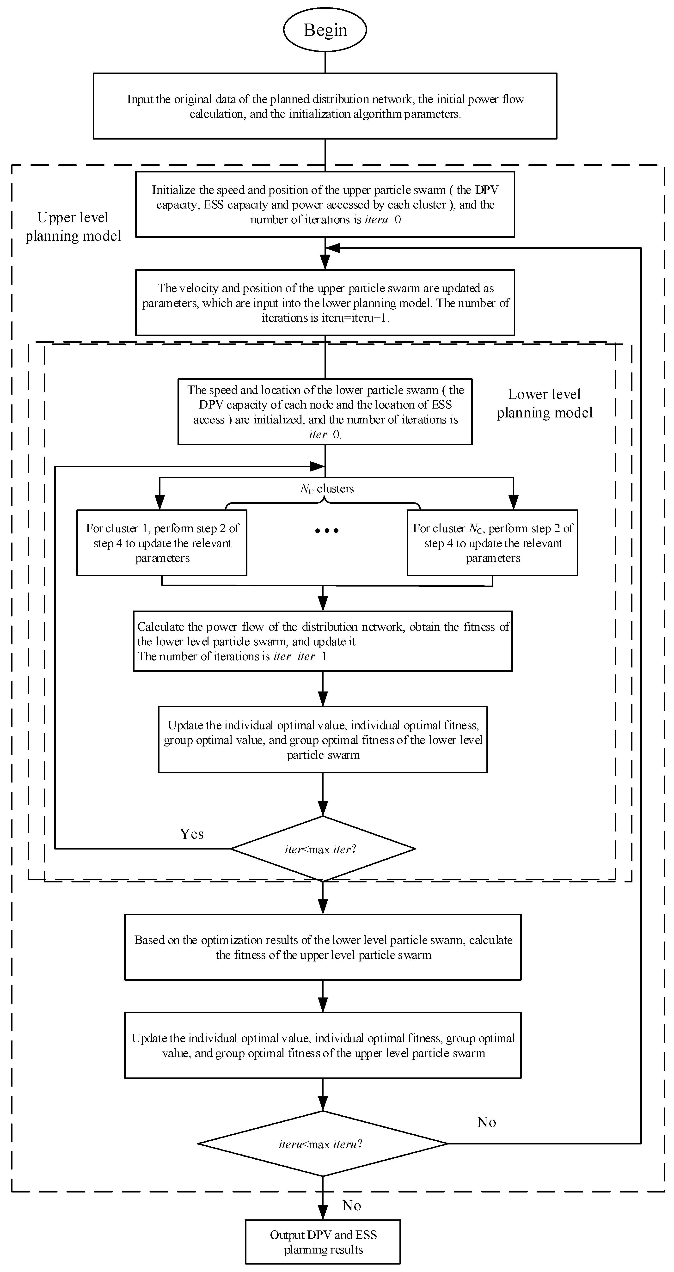
Table A1.
Parameter settings.
Table A1.
Parameter settings.
| Parameter | Valid Values | Parameter | Valid Values |
|---|---|---|---|
| The unit capacity investment cost of DPV/(Yuan/kW) | 5500 | The upper limit of the SOC of NaS | 0.8 |
| The operation and maintenance cost of DPV per unit of electricity generated/(Yuan/kW·h) | 0.3 | The lower SOC limit of NaS | 0.2 |
| DPV service life/year | 20 | Charging efficiency of NaS | 0.9 |
| Investment cost per unit capacity of NaS/(Yuan/kW) | 1260 | Discharge efficiency of NaS | 0.9 |
| Investment cost per unit power of NaS/(Yuan/kW·h) | 1700 | discount rate | 0.06 |
| Operation and maintenance costs per unit of NaS power generation/(Yuan/kW·h) | 0.08 | Photovoltaic power generation subsidy/(Yuan/kW·h) | 0.42 |
| NaS service life/year | 15 | The price of electricity purchased on the main network/(Yuan/kW·h) | 0.55 |
Table A2.
Parameters of each type of ESS.
Table A2.
Parameters of each type of ESS.
| Parameter | NaS | VRB | PSB | VRLA | Li-Ion |
|---|---|---|---|---|---|
| Investment cost per unit of power/(Yuan/kW) | 1650 | 2815 | 1060 | 1980 | 2830 |
| Investment cost per unit capacity/(Yuan/kW·h) | 1270 | 660 | 460 | 980 | 1390 |
| O&M costs per unit of power generation/(Yuan/kW·h) | 0.080 | 0.080 | 0.080 | 0.093 | 0.087 |
| Charge–discharge efficiency | 0.80 | 0.70 | 0.60 | 0.85 | 0.90 |
| Service life/year | 15 | 15 | 15 | 10 | 15 |
Table A3.
DPV-ESS cluster capacity allocation results of each type of ESS.
Table A3.
DPV-ESS cluster capacity allocation results of each type of ESS.
| Planned Scenarios | Cluster 1 | Cluster 2 | Cluster 3 | Cluster 4 | Cluster 5 | Cluster 6 | Cluster 7 | Cluster 8 | Distribution Grids | |
|---|---|---|---|---|---|---|---|---|---|---|
| NaS | PV capacity/kW | 75.723 | 29.146 | 100.715 | 26.236 | 115.155 | 90.560 | 80.205 | 40.921 | 564.652 |
| ESS capacity/(kW·h) | 35.657 | 19.254 | 16.542 | 5.541 | 70.714 | 60.546 | 38.145 | 25.547 | 250.375 | |
| ESS power/kW | 12.031 | 9.734 | 6.045 | 2.651 | 21.175 | 22.916 | 15.450 | 7.755 | 92.572 | |
| VRB | PV capacity/kW | 84.546 | 35.145 | 100.254 | 40.328 | 168.554 | 98.362 | 81.531 | 44.151 | 687.268 |
| ESS capacity/(kW·h) | 76.026 | 22.414 | 25.658 | 53.785 | 283.348 | 86.955 | 45.448 | 30.648 | 604.623 | |
| ESS power/kW | 16.715 | 7.211 | 7.529 | 16.315 | 63.246 | 22.784 | 15.616 | 8.675 | 161.785 | |
| PSB | PV capacity/kW | 141.457 | 50.476 | 128.271 | 20.273 | 371.271 | 160.812 | 88.543 | 88.257 | 1003.726 |
| ESS capacity/(kW·h) | 465.426 | 162.351 | 110.397 | 3.135 | 1217.814 | 445.736 | 78.508 | 358.661 | 2928.325 | |
| ESS power/kW | 109.42 | 30.102 | 36.545 | 1.227 | 243.941 | 91.757 | 23.262 | 81.541 | 589.654 | |
| VRLA | PV capacity/kW | 70.494 | 29.587 | 96.474 | 26.485 | 105.521 | 89.556 | 71.991 | 46.546 | 557.706 |
| ESS capacity/(kW·h) | 15.257 | 13.785 | 14.562 | 3.458 | 65.796 | 52.980 | 20.560 | 23.856 | 209.861 | |
| ESS power/kW | 7.594 | 6.652 | 4.892 | 1.978 | 22.061 | 18.789 | 6.168 | 7.368 | 75.048 | |
| Li-ion | PV capacity/kW | 70.481 | 29.175 | 95.632 | 25.872 | 114.872 | 92.766 | 66.648 | 46.142 | 541.948 |
| ESS capacity/(kW·h) | 15.726 | 13.258 | 10.782 | 2.483 | 64.004 | 62.339 | 4.700 | 21.659 | 193.448 | |
| ESS power/kW | 8.001 | 7.116 | 3.252 | 2.108 | 23.076 | 21.636 | 2.538 | 7.178 | 74.958 | |
References
- Ding, M.; Xu, Z.; Wang, W.; Wang, X.; Song, Y.; Chen, D. A review on China’s large-scale PV integration: Progress, challenges and recommendations. Renew. Sustain. Energy Rev. 2016, 53, 639–652. [Google Scholar] [CrossRef]
- Ding, M.; Wang, W.; Wang, X.; Song, Y.T.; Chen, D.Z.; Sun, M. A review on the effect of large-scale PV generation on power systems. Proc. CSEE (In Chinese). 2014, 34, 1–14. [Google Scholar]
- Zhang, S.; Li, K.; Cheng, H.; Bazargan, M.; Yao, L. Optimal siting and sizing of intermittent distributed generator considering correlations. Autom. Electr. Power Syst. 2015, 39, 53–58. (In Chinese) [Google Scholar]
- Li, Z.; Chen, S.Y.; Fu, Y.; Dong, C.M.; Zhang, J.W. Optimal allocation of ESS in distribution network containing DG base on timing-voltage-sensitivity analysis. Proc. CSEE 2017, 37, 4630–4640. (In Chinese) [Google Scholar]
- Wang, K.; Wang, C.; Yao, W.; Zhang, Z.; Liu, C.; Dong, X.; Yang, M.; Wang, Y. Embedding P2Ptransaction into demand response exchange: A cooperative demand response management framework for IES. Appl. Energy 2024, 367, 123319. [Google Scholar] [CrossRef]
- Zhang, Z.; Hui, H.; Song, Y. Response Capacity Allocation of Air Conditioners for Peak Valley Requlation Considering Interaction with Surrounding Microclimate. IEEE Trans. Smart Grid 2025, 16, 1155–1167. [Google Scholar] [CrossRef]
- Tong, H.; Zeng, X.; Yu, K.; Zhou, Z. A Fault ldentification Method for Animal Electric Shocks Considering Unstable Contact Situations in Low-Voltage Distribution Grids. IEEE Trans. Indnform. 2025, 21, 4039–4050. [Google Scholar]
- Xia, Y.; Li, Z.; Xi, Y.; Wu, G.; Peng, W.; Mu, L. Accurate Fault Location Method for Multiple Faults in Transmission Networks Using Travelling Waves. IEEE Trans. Ind. Inform. 2024, 20, 8717–8728. [Google Scholar] [CrossRef]
- Li, L.; Tang, W.; Bai, M.; Zhang, L.; Lu, T. Multi-objective locating and sizing of distributed generators based on time-sequence characteristics. Autom. Electr. Power Syst. 2013, 37, 58–63. (In Chinese) [Google Scholar]
- Li, K.; Tai, N.; Zhang, S.; Chen, X. Multi-objective planning method of distributed generators considering correlations. Autom. Electr. Power Syst. 2017, 41, 51–57. (In Chinese) [Google Scholar]
- Zhang, S.; Cheng, H.; Li, K.; Bazargan, M.; Yao, L. Optimal siting and sizing of intermittent distributed generators in distribution system. IEEJ Trans. Electr. Electron. Eng. 2015, 10, 628–635. [Google Scholar] [CrossRef]
- Giannitrapani, A.; Paoletti, S.; Vicino, A.; Zarrilli, D. Optimal allocation of energy storage systems for voltage control in LV distribution networks. IEEE Trans. Smart Grid 2017, 8, 2859–2870. [Google Scholar] [CrossRef]
- Muke, B.; Wei, T.; Huang, T. Optimal PV-generation & ES configuration based on virtual partition scheduling and bi-level programming for urban distribution network. Electr. Power Autom. Equip. 2016, 36, 141–148. (In Chinese) [Google Scholar]
- Zheng, L.; Hu, W.; Lu, Q.; Min, Y.; Yuan, F.; Gao, Z.H. Research on planning and operation model for energy storage system to optimize wind power integration. Proc. CSEE 2014, 34, 2533–2543. (In Chinese) [Google Scholar]
- Zhao, B.; Xu, Z.; Xu, C.; Wang, C.; Lin, F. Network partition-based zonal voltage control for distribution networks with distributed PV systems. IEEE Trans. Smart Grid 2018, 9, 4087–4098. [Google Scholar] [CrossRef]
- Ding, M.; Liu, X.; Bi, R.; Hu, D.; Ye, B.; Zhang, J. Method for cluster partition of high-penetration distributed generators based on comprehensive performance index. Autom. Electr. Power Syst. 2018, 42, 47–52. (In Chinese) [Google Scholar]
- Yu, L.; Sun, Y.; Xu, R.; Li, K. Improved particle swarm optimization algorithm and its application in reactive power partitioning of power grid. Autom. Electr. Power Syst. 2017, 41, 89–95. (In Chinese) [Google Scholar]
- Wei, Z. Overview of complex networks community structure and its applications in electric power network analysis. Proc. CSEE 2015, 35, 1567–1577. (In Chinese) [Google Scholar]
- Xue, F.; Chang, K.; Wang, N. Coordinated control frame of large-scale intermittent power plant cluster. Autom. Electr. Power Syst. 2011, 35, 45–53. (In Chinese) [Google Scholar]
- Liu, H.; Fan, B.Y.; Tang, C.; Ge, S.Y.; Wang, Y.; Guo, L. Game theory based alternate optimization between expansion planning of active distribution system and siting and sizing of photovoltaic and energy storage. Autom. Electr. Power Syst. 2017, 41, 38–45. (In Chinese) [Google Scholar]
- Wu, X.; Liu, Z.; Tian, L.; Ding, D.; Yang, S. Energy storage device locating and sizing for distribution network based on improved multi-objective particle swarm optimizer. Power Syst. Technol. 2014, 38, 3405–3411. (In Chinese) [Google Scholar]
- Chi, Y.H.; Sun, F.C.; Wang, W.J.; Yu, C.M. An improved particle swarm optimization algorithm with search space zoomed factor and attractor. Chin. J. Comput. 2011, 34, 115–130. (In Chinese) [Google Scholar] [CrossRef]
- Ding, M.; Liu, X.; Xie, J.; Pan, H. Optimal planning model of grid-connected microgrid considering comprehensive performance. Power Syst. Prot. Control 2017, 45, 18–26. (In Chinese) [Google Scholar]
- Zhao, B.; Xiao, C.; Xu, C.; Zhang, X.; Zhou, J. Penetration based accommodation capacity analysis on distributed photovoltaic connection in regional distribution network. Autom. Electr. Power Syst. 2017, 41, 105–111. (In Chinese) [Google Scholar]
- Xiang, Y.; Wei, Z.; Sun, G.; Sun, Y.H.; Shen, H.P. Life cycle cost based optimal configuration of battery energy storage system in distribution network. Power Syst. Technol. 2015, 39, 264–270. (In Chinese) [Google Scholar]
- Li, P.; Hua, H.; Chen, A.W.; Di, K. Source-load storage coordination partition optimal economic operation of AC/DC hybrid microgrid based on bilevel programming model. Proc. CSEE 2016, 36, 6769–6779. (In Chinese) [Google Scholar]


Disclaimer/Publisher’s Note: The statements, opinions and data contained in all publications are solely those of the individual author(s) and contributor(s) and not of MDPI and/or the editor(s). MDPI and/or the editor(s) disclaim responsibility for any injury to people or property resulting from any ideas, methods, instructions or products referred to in the content. |
© 2025 by the authors. Licensee MDPI, Basel, Switzerland. This article is an open access article distributed under the terms and conditions of the Creative Commons Attribution (CC BY) license (https://creativecommons.org/licenses/by/4.0/).