Abstract
The integration of large-scale distributed photovoltaics (DGPVs) and the generation of distributed photovoltaics (PVs) and loads with distinct characteristics in different transformer areas causes voltage problems in distribution networks, significantly compromising operational reliability and economy. To address this challenge, this study proposes the installation of a relocatable static var compensator (RSVC) to enhance the voltage regulation capability in addition to conventional voltage regulation methods. An RSVC can be deployed at critical nodes of distribution lines to provide continuous adjustable reactive power. RSVCs’ relocation capability in response to seasonal shifts in reactive power demand makes them an effective solution for spatiotemporal load disparities across transformer areas. A bi-level planning framework is established by first generating multiple typical scenarios based on load categories and their seasonal characteristics. The lower level achieves optimal operation in multiple scenarios through the coordination of active–reactive power regulation devices. The upper level employs a particle swarm optimization algorithm to determine the optimal siting and sizing of energy storage and the RSVC, iteratively invoking the lower-level model to minimize the total investment and operational costs. Validation was conducted on a modified IEEE 33-node test system. The results demonstrate that the proposed method effectively mitigates voltage violations caused by DGPVs and spatiotemporal load disparities while significantly enhancing the economic efficiency of distribution networks.
1. Introduction
The integration of large-scale distributed photovoltaics (DGPVs) and the coexistence of photovoltaic (PV) generation and load centers with distinct temporal and spatial characteristics across different distribution transformer areas have introduced significant voltage regulation challenges, seriously compromising the operational reliability and economic efficiency of distribution networks. Field investigations reveal that in some high-penetration regions of China and Europe, more than 30% of feeders have experienced voltage violations exceeding ±5% of nominal voltage levels, directly leading to PV curtailment rates as high as 15% and reactive power losses exceeding 10% under certain scenarios [1].
In recent years, with the support and guidance of national policies, renewable energy has been significantly developed. However, the contradiction between the explosive growth of renewable generators’ capacity and the insufficient flexible regulation capabilities in distribution networks has become increasingly prominent. Notably, significant load disparities among distribution transformer areas, induced by distinct characteristics of industrial loads, ultimately cause spatiotemporal imbalances in 10 kV distribution networks. These imbalances not only hinder local renewable energy consumption but also degrade power quality and economic efficiency when the flexibility regulation capacity is insufficient in distribution networks. Therefore, in order to achieve the rational allocation and utilization of highly intermittent renewable energy, dedicated research on coordinated planning strategies for distribution network flexibility resources carries substantial practical significance in power systems.
At the planning level, various strategies have been explored to enhance the integration of renewable energy through energy storage system (ESS) deployment. Early efforts, such as that in [2], introduced distributed ESS planning models that incorporate wind–PV uncertainty, guiding deployment across different integration stages. Subsequent research expanded on this foundation; for instance, the authors of [3] focused on minimizing transmission losses and improving utilization efficiency by strategically placing battery energy storage systems within transmission and distribution grids. Addressing system flexibility under extreme conditions, the authors of [4] developed a joint planning framework that combined smart soft open points (SOPs) with an ESS to optimize reliability and economic performance.
Meanwhile, multi-objective optimization techniques have gained traction. A notable example is the genetic algorithm-based configuration model proposed in [5], which jointly optimized ESS and static var compensator (SVC) allocation to enhance voltage stability and cost efficiency. Further studies, such as [6], emphasized the role of multi-scale storage technologies such as batteries and supercapacitors in reducing investment costs under uncertainty. Additionally, the authors of [7] proposed a hybrid configuration strategy that integrated energy storage with reactive power compensation to balance flexibility, voltage quality, and cost-effectiveness under varying renewable penetration levels. Building on this, the authors of [8] introduced a coordinated grid–load–storage planning scheme that leverages demand-side flexibility resources to further enhance the distribution network’s adaptability to renewable energy fluctuations, opening new avenues for improving system flexibility.
From an operational perspective, research has increasingly emphasized real-time control strategies and flexible device coordination. For example, the authors of [9] proposed regulating the active and reactive outputs of PV inverters to mitigate voltage violations at grid connection points. Complementary to this, the authors of [10,11] demonstrated that the rapid-response capabilities of an ESS significantly improve the voltage quality.
More comprehensive strategies include the bi-level optimization framework proposed in [12], which leverages an ESS to absorb PV output fluctuations while coordinating SVC and inverter actions to minimize losses and deviations. Similarly, the authors of [13] introduced a robust optimization model that accommodates wind power variability and capitalizes on energy storage’s voltage regulation capacity.
Further advancements were seen in [14,15], where zonal voltage control and grid-forming energy storage were used to address medium- and low-voltage stability issues. In addition, the authors of [16] proposed a coordinated operation model integrating conventional regulation equipment with distributed storage units, enabling more effective reactive power management across voltage levels.
However, the aforementioned studies focused on the characteristics of different flexible devices or addressed the impacts of wind and solar uncertainty, but rarely considered the influence of significant seasonal load differences within and between transformer areas on the distribution network planning and economic operation.
This study takes a certain southwestern province of China as an example. After the integration of DGPVs, the connected 10 kV distribution line experienced persistent overvoltage issues during periods of high solar irradiance, with the voltage reaching up to 277 V. This severe overvoltage condition rendered daytime electricity consumption virtually impossible for users. The 10 kV line was supplied by a 110 kV substation. Among the 41 distribution transformers monitored by the distribution network voltage monitoring system, 26 exhibited high-voltage conditions. The average voltage compliance rate for the transformer zones was 97.79%, with an average overvoltage rate of 2.092% and a maximum mean voltage of 240.4 V. The line supplies 1996 low-voltage customers, primarily residential loads. With a safe current-carrying capacity of 160 A, the maximum operating current under normal conditions is 77.58 A (1.33 MW), indicating relatively light loading with a peak load rate of 48.49%. Significant PV output can trigger overvoltage conditions. Due to the inherent intermittency and stochastic nature of solar energy, PV integration significantly impacts the power quality and stability in distribution networks. The increasing PV penetration alters traditional power flow patterns, potentially causing reverse power flow that elevates voltage at network endpoints. In severe cases, this may lead to system instability, highlighting the importance of addressing voltage impacts from distributed PV integration.
In regions with such characteristics, the difficulty in planning is increased when a balance of higher reliability and economic efficiency is required.
Based on this, we propose a novel bi-level planning method for an ESS and RSVC in distribution networks to address the large seasonal load differences in transformer areas. An RSVC is basically the sharing of a group of SVCs in different load scenarios. A group of SVCs, which can be decommissioned, transported to different locations, and re-integrated into the distribution feeders, was planned due to the seasonal and temporal characteristics of the load at different transformer areas. Therefore, multiple transformer areas share the group of SVCs, and the requirements of both the economic and voltage quality of customers are met. The proposed methodology also integrates a DGPV and an ESS for active power balance coordination, synergistically combined with an on-load tap changer (OLTC) transformer and an RSVC, while utilizing the residual capacity of the DGPV and ESS inverters to solve the problem of numerous low-voltage transformer areas and the seasonal nature of low-voltage periods.
By evaluating the benefits of ESS and DGPV participation in reactive power and voltage regulation, as well as the investment in an ESS and RSVC, the feasibility of the proposed method is verified from both planning and operational perspectives.
The remainder of this paper is structured as follows: Section 2 presents a comparative evaluation and practical considerations for deploying RSVCs; Section 3 describes the proposed bi-level planning model, including upper- and lower-level formulations; Section 4 outlines the solution methodology based on particle swarm optimization (PSO) and details the RSVC deployment logic; Section 5 validates the proposed method through simulation studies on a modified IEEE 33-node system under different seasonal load scenarios; and Section 6 concludes the paper with key findings and potential directions for future research.
2. Comparative Evaluation and Practical Considerations of RSVC Deployment
2.1. Comparative Analysis Between RSVC and Conventional FACTS Devices or Smart Inverters
To better evaluate the cost-effectiveness and technical applicability of the proposed RSVC, a comparative analysis was conducted against conventional devices such as fixed SVCs and advanced FACTS technologies such as SVGs or smart inverters. As summarized in Table 1, RSVCs offer significantly improved economic performance, especially in rural distribution networks, where seasonal or temporary voltage issues are frequent. RSVCs achieve a lower unit investment, higher utilization, and faster investment recovery through their flexible deployment and reuse. Their response time and service life are sufficient to meet the typical compensation needs in weak grid environments.

Table 1.
Technical and economic comparison of voltage regulation devices.
Moreover, RSVCs provide deployment flexibility that fixed devices cannot match. They are particularly suited to temporary, mobile, or emergency regulation tasks, minimizing the need for redundant fixed infrastructure. Their adaptability to sustained load changes lasting over 15 days makes them more efficient under scenarios where grid reinforcement is economically unviable. In such contexts, RSVCs stand out as a technically feasible and economically sound solution.
2.2. Operational Constraints and Practical Deployment Considerations of RSVC
Despite its advantages, RSVC deployment also involves practical constraints. According to actual engineering cases in a southwestern region, a complete relocation over a distance of 80 km can be executed within 31 h, including live disconnection, transportation, reconnection, and commissioning. The process requires less than 10 h of technical operation, with the remainder allotted to safety management. RSVCs are designed for live operation, compact layout, and modular construction, incorporating safety-enhanced interfaces and self-adaptive logic to support frequent mobile deployment.
Such mobility allows RSVCs to be relocated ahead of seasonal demand surges or during temporary low-voltage incidents. Their operation typically targets sustained load variations of 15 days or longer, which aligns with the load characteristics in many rural areas. However, factors such as land availability, the scheduling of safe operating periods, relocation fatigue, and interconnection coordination must still be addressed during system planning. These constraints do not offset the strategic advantages RSVC offers but underscore the importance of realistic deployment frameworks when integrating mobile devices into rural network regulation strategies.
3. A Bi-Level Optimal Configuration Model for Energy Storage Systems and RSVCs in Distribution Networks
A bi-level optimization framework is proposed to address the seasonal low-voltage issues in different distribution transformer areas and overvoltage problems induced by the high penetration of DGPVs. The upper-level optimization framework establishes the optimal siting and sizing of an ESS and SVC through cost-minimization objectives. The lower-level optimization focuses on the operation of the distribution network under multiple typical load scenarios. The operational costs of the distribution network under representative scenarios are minimized while adhering to operational constraints, including voltage deviation limits, branch flow limits, power balance requirements, and equipment capacity constraints. Based on the optimal locations and capacities of an SVC in each typical scenario, the total capacity and capacity allocation of an RSVC can be determined.
3.1. The Upper-Level Optimization Model
3.1.1. The Objective Function
The upper-level objective aims to minimize the total cost, including the investment and O&M costs of an ESS, of the SVCs, for reactive power compensation, and the operational costs of the distribution feeder, , as given by (1) to (3):
where is the investment in an ESS, quantified as a specified proportion of the ESS’ rated power and capacity as given by (3). and are the cost coefficients related to the rated power and capacity of an ESS, respectively. is the operational cost of the ESS obtained from the lower-level optimization model. and are the rated power and rated capacity of the ESS, respectively. is the set of ESSs that are to be configured. and denote factors to scale the total investment of an ESS and SVCs to the observed time. When the scaling factor equals zero, it indicates that the corresponding device is not deployed.
in (1) represents the reactive power compensation cost, which is given by (4).
where is the reactive power compensation cost of the total SVC capacity. is an SVC’s capacity at bus i. is the total number of nodes in the distribution network. , , , and are configuration coefficients [17].
in (1) represents the system operational costs.
where denotes the operational cost of network losses under multiple scenarios. represents the unit network loss cost (CNY/kWh). indicates the network loss (kWh) of the optimal operating scheme in the mth typical scenario, which is calculated by the lower-level optimization model. is the duration of the mth typical scenario. G denotes the total number of scenarios.
3.1.2. Constraints
- (1)
- Installation constraint for ESS components:
- (2)
- The SVC capacity is directly proportional to the area covered, so the single SVC capacity needs to be constrained, as given by (7):
- (3)
- Total SVC quantity constraint:
3.2. Lower-Level Optimization Model
The lower-level model takes the siting and sizing decisions of the ESS and SVC from the upper-level model. By coordinating the active–reactive power regulation via PV inverters, SVCs, and OLTC, it optimizes the distribution network’s operational economy, voltage quality, and CO2 emissions.
3.2.1. The Objective Function
The objective of the lower-level model is given by (9):
where denotes the network loss cost. represents the feeder’s electricity purchasing cost. indicates the PV curtailment penalty. corresponds to the PVs’ operational cost. represents the ESS’ operational cost. defines the regulation cost of all reactive compensation resources. characterizes the CO2 emissions’ cost.
- (1)
- Distribution network loss costs, :
- (2)
- Electricity purchasing costs, :
- (3)
- Solar curtailment cost :
- (4)
- DGPV’s operational cost, :
Through the advanced inverter control scheme, the DGPV can also generate or absorb reactive power; however, it poses significant thermal stress to internal components. Concurrently, increased the reactive power output induces an increase in the inverter’s power losses, consequently elevating operational expenditures and inducing efficiency deterioration. Therefore, a unit power operation cost metric is adopted to quantify the comprehensive operational cost of the DGPV’s inverter.
where is the per unit operating cost of a DGPV. is the active power generation of a DGPV at time t. is the reactive power generation of a DGPV at time t.
- (5)
- Operating cost of ESS (storage power dispatch cost):
The charge–discharge cycles of an ESS inevitably incur energy loss, and these are also used as an indicator of the ESS’s remaining life. Therefore, it is imperative to incorporate unit power operational costs to quantify the comprehensive operational costs generated by ESS operations.
where denotes the unit power operational cost of the ESS. and indicate the charging and discharging power at time t, respectively.
- (6)
- Voltage regulation sequence:
When power inverters of DGPVs and ESSs participate in reactive voltage regulation, the coordination between conventional voltage regulation methods and flexible regulation approaches needs to be considered. Converters can change reactive power injection or absorption continuously, whereas traditional voltage regulation devices such as an OLTC operate through discrete rule-based control mechanisms. Without coordination, there may be ineffective utilization of the lower-level regulating equipment, which can pose the risk of overloads in continuously adjustable reactive power compensation devices.
Based on this, the following cost function was designed as follows:
where denotes the tap’s position of the OLTC at time t. , , and represent the reactive power output/absorption from the ESS, PV inverter, and SVC at time t, respectively. denotes the indicator function; it outputs 1 when its argument is non-zero. is the weighting coefficient used to maintain comparability between this cost term and the other components in the objective function. The exponential function characteristic ensures prioritized regulation through OLTC adjustment.
- (7)
- CO2 emission cost, :
This study employed the life cycle assessment method to calculate the carbon emission intensity of each generation unit [18]. The production, transportation, construction, operation, and decommissioning processes of renewable energy units contribute to greenhouse gas emissions. Consequently, the potential impacts of renewable energy generation technologies on carbon emission costs must be systematically evaluated.
where denotes the unit penalty cost for carbon emissions. represents the total carbon emissions. indicates the per unit carbon emission intensity of DGPVs’ generation. refers to the per unit carbon emission intensity of electricity purchased from the main upstream grid.
3.2.2. Constraints
- (1)
- ESS operational constraints:
- (2)
- OLTC operational constraints:
- (3)
- SVC reactive power compensation capacity constraint:
- (4)
- ESS’s active and reactive power output constraint:
The maximum available capacity constraint of the ESS is formulated as follows:
where and denote the active and reactive power outputs injected by the ESS at node i during time t, respectively. is the maximum available capacity of the ESS integrated at node i.
- (5)
- Power flow constraint:
Power flow constraints comprise active and reactive power balance constraints. Considering the integration of an ESS, the active power balance constraint is formulated as follows:
where is the active power (kW) from the generator or distributed PV at node i at time t. In the simulation, node 0 is the starting end of the 10 kV feeder. is the active power from the grid of upper voltage level. In operation, reverse power transmission to the higher voltage level is not allowed. Therefore, must be greater than or equal to 0. is the active power (kW) consumed by the loads at node i at time t. and are the voltages at nodes i and j, respectively. and denote the conductance and susceptance between nodes i and j, respectively. is the phase difference between nodes i and j at time t.
We consider the reactive power balance constraint as
where is the reactive power (kVar) emitted by the generators or distributed PV at node i at time t. is the reactive power (kVar) emitted by the SVC at node i at time t. is the reactive power (kVar) consumed by the load at node i at time t. represents the reactive power (kVar) emitted by the energy storage device at node i at time t, which is negative when the storage device absorbs the reactive power.
- (6)
- Distribution network operational constraints:
The safe operation constraints of distribution networks include the voltage safety and current safety constraints:
where and are the nodal voltage limits. and are the line current limits.
4. Optimization Model Solution Process
4.1. Optimization Model
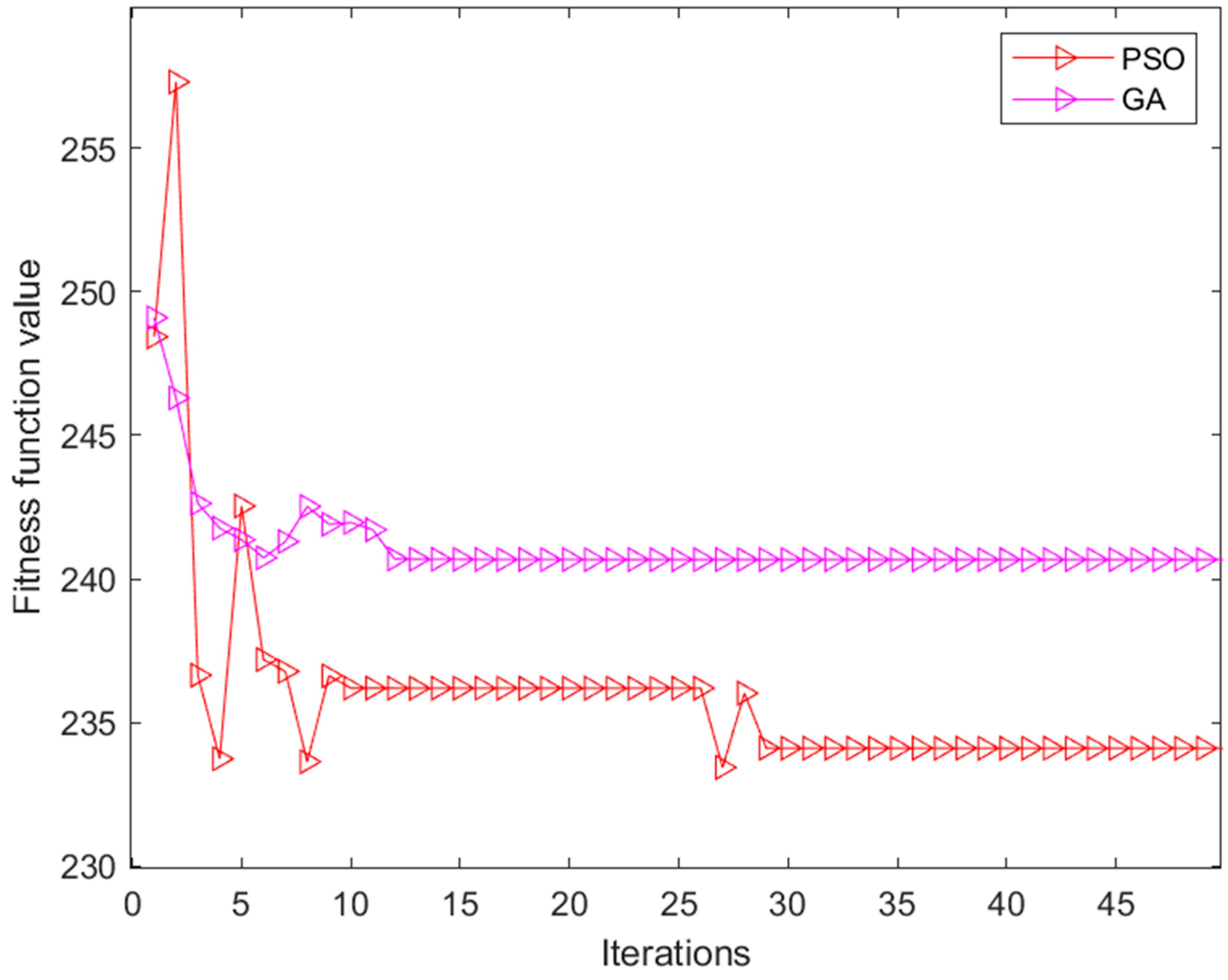
To solve the joint optimization problem of RSVC and ESS configurations, this study employed the particle swarm optimization algorithm, which balances global exploration and local convergence through dynamic parameter tuning. The PSO was specifically chosen for its superior global search capability and fast convergence, as evidenced by the comparison of the convergence curves of the PSO and genetic algorithm (GA) given in Figure 1. The PSO converges rapidly, typically stabilizing by around iteration 5, with the fitness value decreasing steeply early on and quickly reaching a lower value. In contrast, the GA initially converges faster but eventually becomes trapped at a local optimum, showing a plateau effect and failing to improve further despite the initial drop.
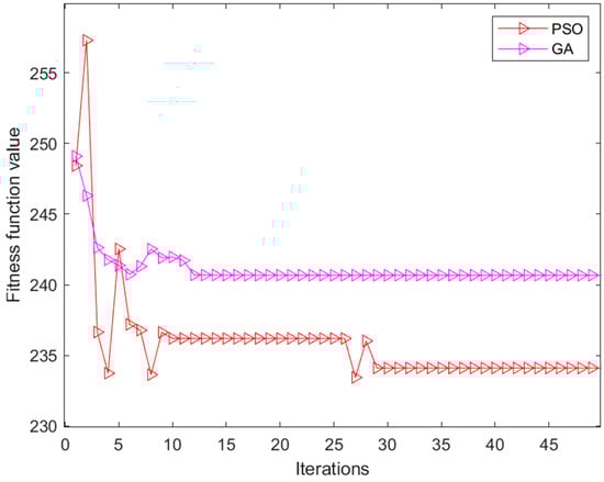
Figure 1.
Multi-objective optimization iterative curve.
The inertia weight (ω) in the PSO linearly decreased from 0.9 to 0.4 over the course of iterations. This dynamic adjustment facilitates a broad search in the early stages, ensuring global exploration while enabling faster convergence toward the optimal solution in later iterations. Both the cognitive (c1) and social (c2) acceleration coefficients were set to 2.0, which ensures a balanced influence of individual and group experience on particle velocity updates, thus improving both exploration and local optimization.
To evaluate the convergence performance, multiple trials were conducted. The convergence curves of the fitness values indicate that the PSO stabilized quickly within 50 iterations. Additionally, the PSO algorithm was executed 20 times independently, and the standard deviation of the best solution values remained below 1.2%. These findings confirm the suitability of the PSO for solving the bi-level planning problem under scenario-based uncertainty, with a notably faster and more reliable convergence to the global optimum compared to the GA. Furthermore, the robustness of the PSO across multiple runs highlights its effectiveness in providing stable solutions under varying initial conditions and parameter settings, validating its computational performance and reliability.
4.2. Process
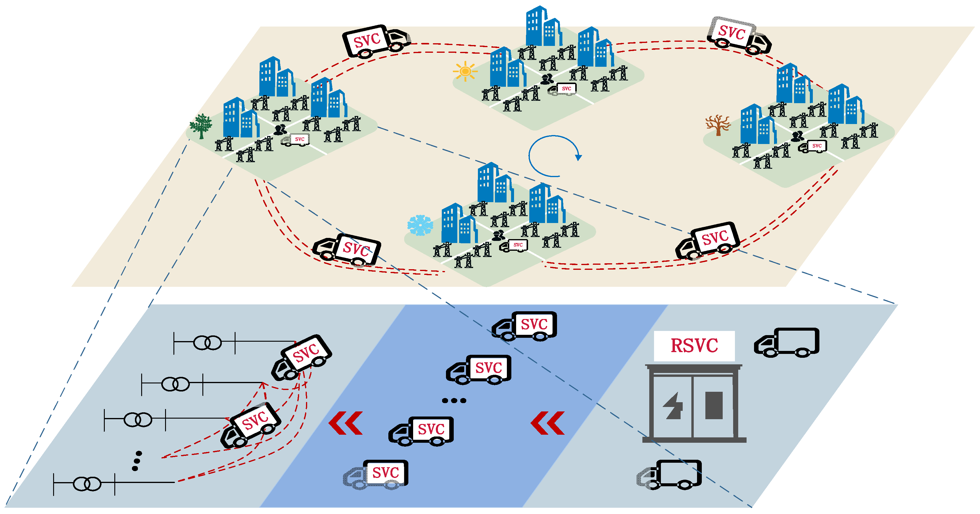
Inspired by the operation mode of mobile energy storage vehicles, RSVCs can change their integration points across different distribution transformer areas according to time-varying reactive power demands. This approach allows multiple distribution areas with asynchronous voltage regulation needs to share limited SVC resources more flexibly and cost-effectively. It forms the foundation of the proposed planning model, enabling the spatial and temporal coordination of reactive support under seasonal and operational variability. Figure 2 illustrates the interconnection concept of the RSVC mobile reactive power compensation.
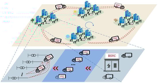
Figure 2.
Concept diagram of mobile reactive power compensation.
Based on this concept, the solution process of the bi-level planning model developed in Section 1 is illustrated in Figure 3. First, multiple DGPV and load scenarios under typical operating conditions were generated by considering the seasonal characteristics of the DGPV and loads at different nodes. Subsequently, the upper-level planning model employed a PSO algorithm to determine the optimal siting, sizing, and power ratings for the ESS and SVCs. The planning decisions that were obtained for the ESS and SVCs were then passed to the lower-level model. The lower-level model optimized the daily dispatch schedules by minimizing the total operational cost in typical scenarios. These operational results were fed back to the upper-level model. Finally, the upper-level model performed a fitness evaluation using the PSO algorithm based on the planning configurations and scenario-based operational costs, iteratively updating solutions until convergence to optimal planning decisions.
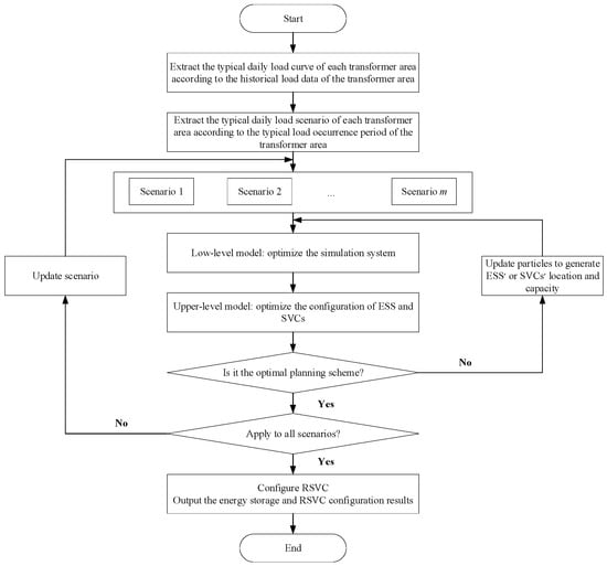
Figure 3.
Algorithm flowchart.
4.3. RSVC Configuration
The primary objective of deploying an RSVC is to share the reactive compensation capacity when loads at different low-voltage transformer areas have quite different load curves during different seasons or time spans. The optimization method given in Section 2 suggests the installation of different groups of SVCs under different typical scenarios, as given in (27):
where represents the capacity and installation location of the kth SVC in the mth scenario. represents the optimal capacity, and represents the installation location. The subscript m represents the scenario, and the superscript k represents the kth SVC installed under scene m, which satisfies . The set of SVCs under scene m is sorted in descending order of capacity; that is, .
The total capacity of the RSVC needed is then given by (28).
5. Simulation Analysis
5.1. Test System Introduction
The mountainous terrain of province A (a certain southwestern province in China) results in a long power supply radius and a complex branching structure of the power grid. Relying on agriculture and tourism as economic pillars, the region’s load exhibits significant load fluctuations influenced by seasonal factors, including tourist peaks, spring irrigation, and specific load types, such as tea processing and tobacco curing. The total load at the 10 kV feeder and the loads at different load voltage distribution transformer areas show distinct patterns and cycles influenced by industrial operations, seasons, and long- and short-term holidays. For example, due to the influence of the wave of going back to work and school in February, the number of tourists decreases, leading to a significant decline in electricity load. April is the peak season for tea production, and July to November is the peak season for cured tobacco production, resulting in a significant increase in the power load. The daily maximum load difference across the province can reach up to 11,000 MW, and the extreme difference between the daily loads is also as high as more than 5000 MW, accounting for 44% and 20% of the annual peak load, respectively.
In rural 10 kV distribution networks characterized by long feeder lengths and weakly meshed structures, voltage regulation challenges are particularly pronounced due to highly seasonal and cyclic load variations. This issue is especially evident in certain southwestern provinces of China, where the rural grid topology closely resembles that of the IEEE-33 bus system. For instance, in the study area, a typical 10 kV feeder spans up to 44.027 km and supplies 41 distribution transformer areas. Owing to confidentiality constraints, this study adopts the IEEE-33 bus test system as a representative model in place of the actual grid topology and operational data. Therefore, in this study, we used the IEEE 33-node system as a test system. To validate the effectiveness of the proposed bi-level optimization strategy and algorithm for distribution networks considering seasonal load variations in transformer areas, simulations were conducted on a modified IEEE 33-node distribution system, whose topological structure is illustrated in Figure 4. The system parameters were defined with base values: UB = 12.66 kV, SB = 1 MVA. An OLTC transformer was installed at node 0, with its tap adjustment range set to 1 ± 3 × 1%. PV generation units with rated capacities of 1.35 MW, 0.5 MW, 1.2 MW, and 1.35 MW were connected at nodes 14, 21, 24, and 28, respectively. The rated solar intensity was set to be 1000 W/m2. Through a simulation analysis, the optimal sizing and placement of the ESS and SVCs were determined. Furthermore, the capacity allocation and total capacity of RSVCs were optimized based on mobile RSVC deployment principles.
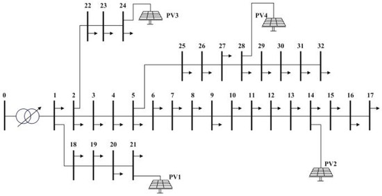
Figure 4.
Modified IEEE 33-node test system.
5.2. Typical Load Curve
Rural power systems in a certain southwestern province of China exhibit diversified load characteristics across 10 kV distribution transformer areas, demonstrating significant seasonal and diurnal fluctuation disparities. However, the aggregated feeder-level load manifests homogeneous patterns across seasonal and temporal dimensions.
5.2.1. Differential Distribution Transformer Area Load Curves
To reflect the spatiotemporal diversity of rural loads in the 10 kV distribution networks of a certain southwestern province of China, typical load scenarios were derived based on historical transformer-area-level load data. First, distribution transformer areas were preliminarily classified by dominant load types—such as tourism, tea processing, and tobacco curing—according to their seasonal and diurnal usage patterns. Annual load curves sampled at 15 min intervals were then collected for each type. These curves were normalized and subjected to K-means clustering using the Euclidean distance to identify representative profiles, with the optimal number of clusters determined using the elbow method [19]. To further capture short-term load fluctuations, wavelet decomposition was applied to enhance the temporal resolution. Representative daily curves were then extracted from each cluster and used as typical load scenarios for subsequent planning analysis.
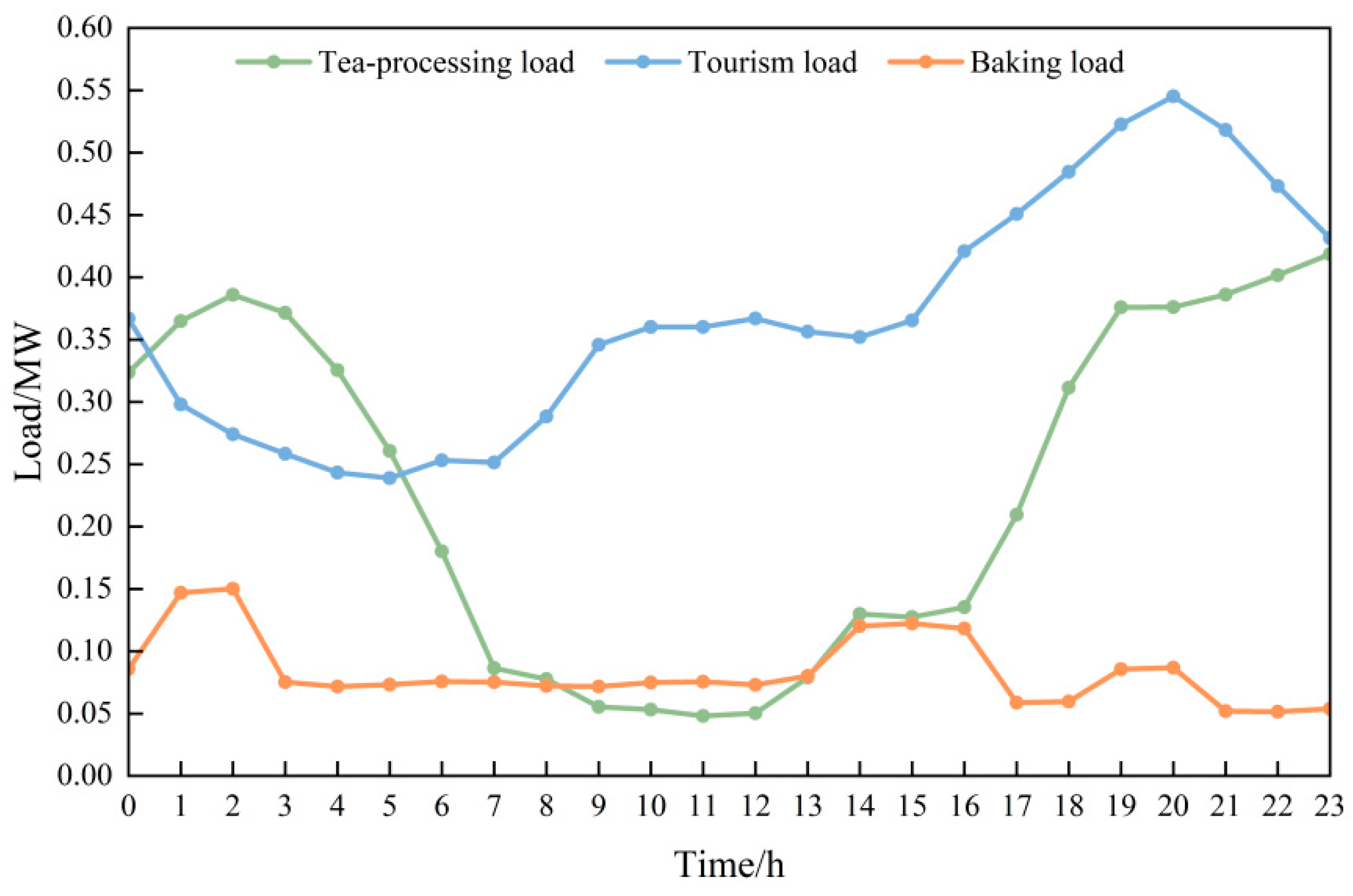
Three typical load profiles of 10 kV distribution transformer areas were selected, including the tourism peak load during the Spring Festival, the tea-processing load in April, and the tobacco-curing load from July to November. The daily load curves for these typical load scenarios are illustrated in Figure 5. The nodal locations corresponding to each load scenario are summarized in Table 2. The loads at the nodes not mentioned in Table 3 were chosen to be the same as the standard IEEE 33-node test system.
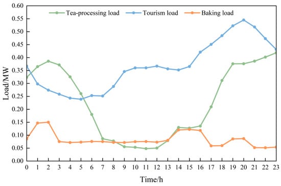
Figure 5.
Daily load curve of the typical load in each time period.
Table 2.
Typical load node location in each time period for the 33 nodes.
Table 3.
Model parameters.
The simulation parameters were obtained by organizing the relevant data and are summarized in Table 3 [20].
As illustrated in Figure 5, significant disparities exist among the load curves of tourism-related, tea-processing, and tobacco-curing loads. During the period from 01:00 to 08:00, the tourism-related load remains at relatively low levels, reaching its daily minimum at 05:00. A marked increase commences at 15:00, culminating in the peak load at 20:00. The Spring Festival holiday period represents a minor tourism peak in winter, which increased hotel occupancy rates due to tourist influx lead to elevated night-time electricity consumption, while the daytime demand remains comparatively low, collectively manifesting pronounced peak–valley differentials. The tea-processing load emerges during the April tea season. Although its daily load profile imposes limited impact on the grid overall, the concentrated electricity consumption in tea-growing areas—where daytime harvesting and nighttime processing operations coincide—induces rapid load surges during specific periods, exerting notable effects on the local grid infrastructure and power quality. The daily load curves distinctly reveal an inverse relationship between tea-season and non-tea-season load patterns: the former is characterized by lower daytime and higher night-time loads, whereas the latter exhibits the opposite trend.
During the tobacco-curing cycle from July to November in a certain southwestern province of China, peak thermal drying loads predominantly occur during the forced ventilation phase, late wilting stage, and large rolling stage. The load fluctuation patterns demonstrate substantial similarity across the curing phases, with maximum values not exceeding 40 kW. In the case study design, the curing loads were exclusively distributed at nodes 11, 16, 20, and 31, resulting in a cumulative load below 150 kW. The tobacco-curing load exhibited distinct fluctuation characteristics. During forced ventilation, accelerated airflow induces significant thermal demand increments. The late wilting stage witnesses intensified moisture evaporation from tobacco leaves, necessitating enhanced heat supply from the heat pump drying system, which consequently elevates the load levels. In the large rolling stage, leaf curling accelerates the drying process, thereby further amplifying the thermal loads.
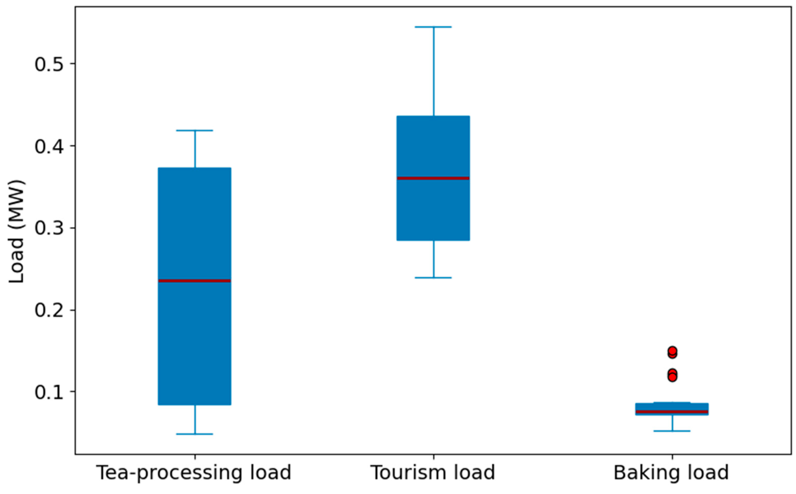
The box plot in Figure 6 clearly presents the variability and distribution characteristics of each load type, highlighting the distinct load fluctuation patterns between the tourism, tea-processing, and tobacco-curing operations. The median line and interquartile range effectively capture the central tendency and dispersion, while the outliers reflect occasional peak loads, particularly in baking operations. This visualization aids in understanding the diverse loading profiles and their potential impacts on grid stability.
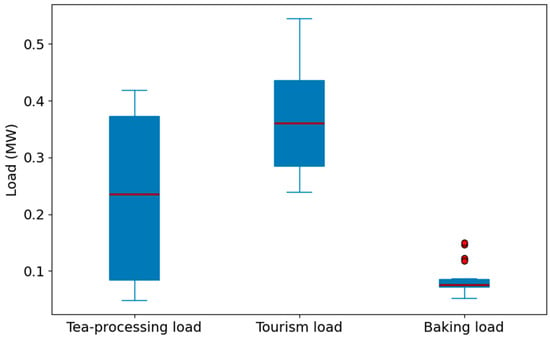
Figure 6.
Variability of the load data.
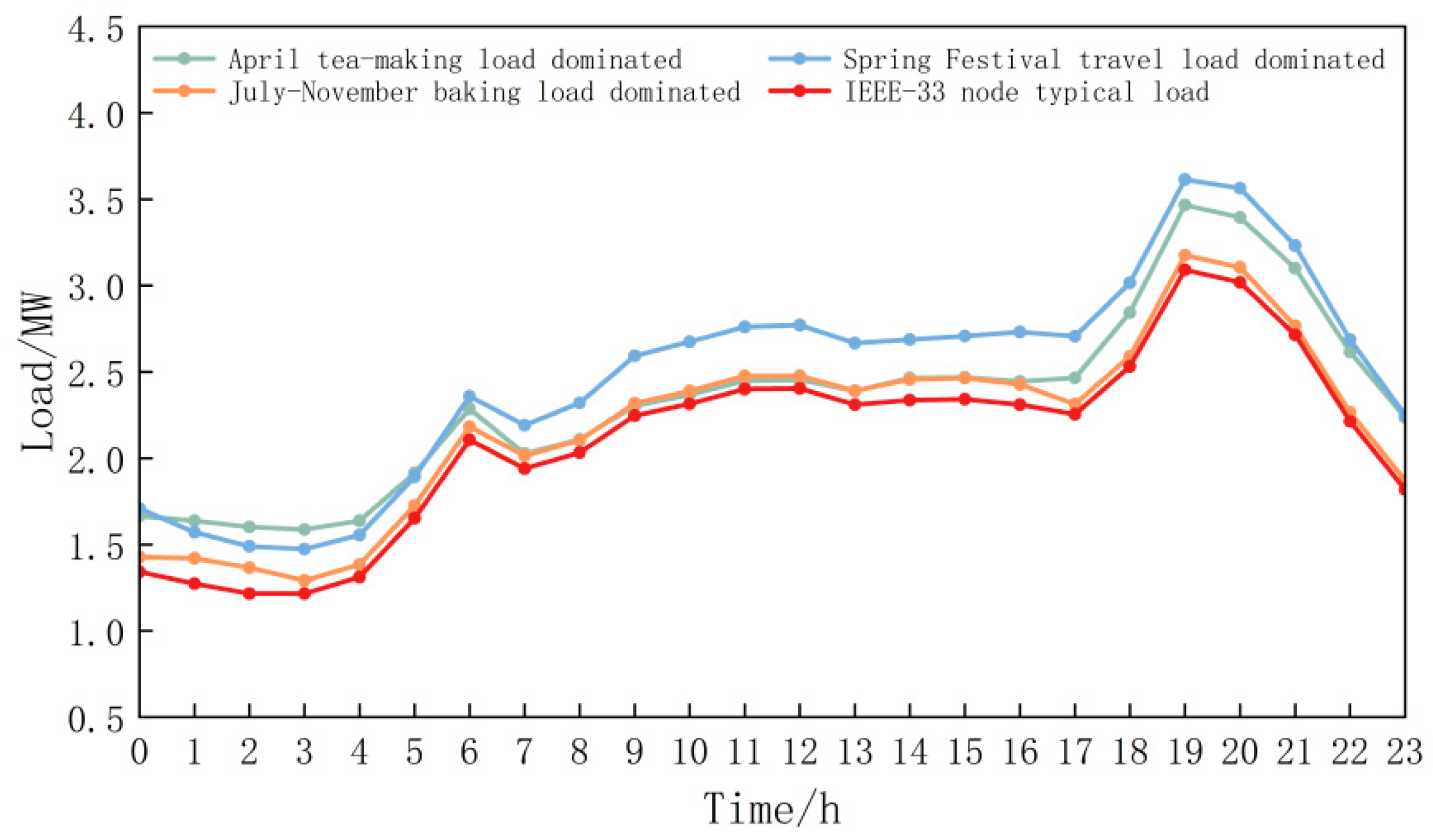
5.2.2. Total Load Curve
By superimposing the conventional nodal loads with the time-variant load profiles specified in Table 3, the aggregate load curves for 10 kV feeders were derived under three characteristic scenarios, as depicted in Figure 7. To mathematically express the typical daily load curve, the following equation is used:
where is the typical daily load at time t. is the base load at time t. is the load variation of the ith characteristic scenario at time t. n is the number of characteristic load scenarios.
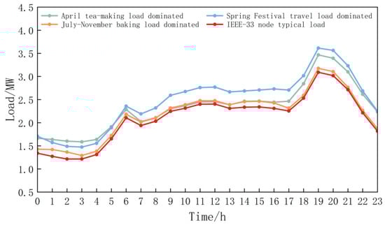
Figure 7.
Typical daily load curve of the 10 kV outgoing line in different scenarios.
This formulation accounts for the superposition of the base load and time-variant characteristics, ensuring that the derived curve accurately reflects the dynamic load variations in different scenarios.
The comparative analysis in Figure 5 and Figure 7 reveals that while the macro-scale contour similarity of the total load curves persists across temporal scenarios, significant divergences emerge in nodal load characteristics, particularly in peak–valley differentials and profile shapes.
In summary, by analyzing the seasonal and daily fluctuation characteristics of different transformer area loads, it was demonstrated that these typical scenarios encompass various load types that may impose stress on the power grid. The peak tourist load is associated with holiday consumption, the tea-making load corresponds to specific tea-picking seasons, and the tobacco-curing load aligns with agricultural production cycles. These load fluctuations impact the grid’s load demand, peak-to-valley difference, and voltage control. The significant peak-to-valley disparity in tourist load may place high demands on the power system during certain periods, necessitating the deployment of additional energy storage and reactive power compensation devices to ensure voltage stability and load balance. Seasonal fluctuations in the tobacco-curing load can lead to unstable load demands, all of which need to be considered over the entire life cycle.
5.3. Analysis of the Planning Results
To evaluate the effectiveness of the proposed ESS and mobile RSVC bi-level planning framework compared to conventional fixed SVC configurations, as well as the performance of photovoltaic systems in active power-only versus combined active–reactive power regulation for addressing voltage issues in modern distribution networks, three operational cases were proposed with distinct flexibility resource participation in active/reactive power planning. For each case, three typical nodal load profiles from different time periods were input to obtain the planning results of the ESSs and RSVCs.
Case 1: DGPVs generate active power only without participating in voltage regulation; ESSs are deployed without reactive power regulation capability.
Case 2: DGPVs participate in both active and reactive power regulation; RSVCs are implemented without energy storage deployment.
Case 3: DGPVs engage in integrated active–reactive power regulation with the simultaneous deployment of ESSs and RSVCs.
The simulation platform MATLAB 2021a was adopted, and the annual planning results of the ESSs and RSVCs under each operational scenario are shown in Table 4.
Table 4.
Annual planning results in different scenarios.
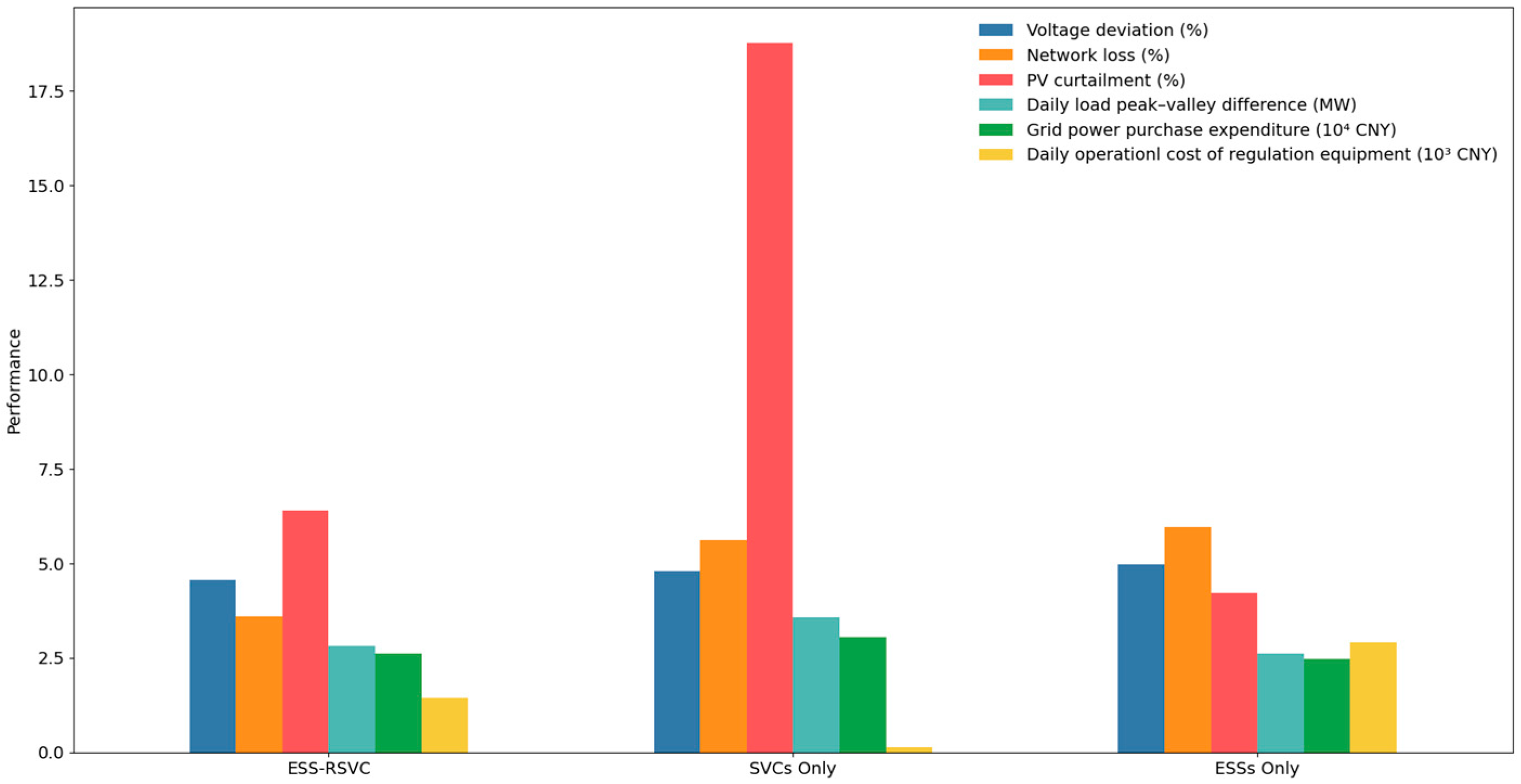
Under identical operating conditions, when employing only conventional voltage regulation equipment—including OLTC and fixed SVCs—the DGPVs operated exclusively in the active power injection mode, providing no voltage regulation support. In this configuration, the voltage quality maintenance relied entirely on the SVC units. Seven SVCs were strategically installed at nodes 8, 10, 15, 17, 21, 29, and 31, with rated capacities of 122 kVar, 110 kVar, 178 kVar, 156 kVar, 190 kVar, 217 kVar, and 202 kVar, respectively. While this approach ensured voltage compliance under certain conditions, it demonstrated limited adaptability and efficiency, particularly under high PV penetration. Notably, this configuration resulted in a network loss rate of 5.62% and a PV curtailment rate of 18.77%, indicating suboptimal performance, as shown in Figure 8.
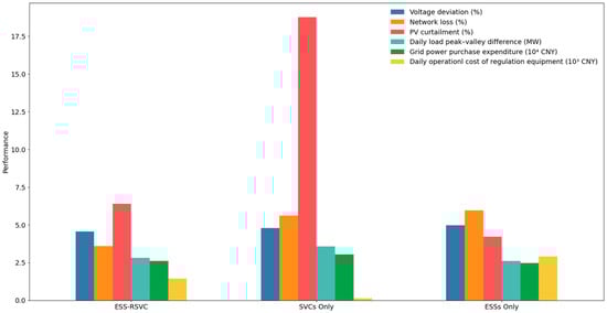
Figure 8.
Comparison of voltage regulation methods.
To compare the overall performance among the evaluated scenarios, six key indicators were analyzed: voltage deviation, network loss, PV curtailment, load peak–valley difference, grid power purchase expenditure, and the daily operational cost of regulation equipment. Case 3 (ESS-RSVC) consistently achieved the best balance across all metrics, indicating superior overall performance.
In contrast, the scenario configured with an OLTC and ESSs demonstrated effective peak–valley load shifting, minimal PV curtailment, and reduced power purchase cost. However, due to the absence of reactive power support, it exhibited relatively poor performance in terms of voltage deviation, network loss, and daily operational cost. Conversely, the configuration based on an OLTC combined with multiple fixed SVC units effectively improved the voltage compliance and alleviated the low-voltage issues during heavy-load periods. In this setting, seven SVCs with substantial capacities were deployed at various nodes. Nevertheless, this static configuration resulted in significantly higher PV curtailment, peak–valley load difference, and power purchase expenditure, as it lacked the energy-shifting flexibility provided by ESSs and could not dynamically respond to fluctuations in renewable generation and load demands.
These results highlight the advantage of the proposed coordinated planning method in case 3, demonstrating its capability to synergistically manage active and reactive power through ESS and RSVC deployment. This comprehensive improvement underscores the effectiveness and robustness of the proposed bi-level planning strategy in modern distribution networks with high PV penetration.
As demonstrated in the in-depth comparative analysis of cases 1–3, case 1 effectively reduces the electricity procurement costs from the main grid by leveraging the ESS for charging during periods of high PV generation and discharging during heavy-load periods without solar power. However, high PV penetration rates combined with distribution network constraints prohibiting reverse power flow necessitate PV curtailment during peak generation periods and fail to fully resolve the low-voltage issues in heavy-load conditions. Case 2, which employs only relocatable static var compensators, incurs higher electricity procurement costs from the main grid. The implementation of RSVCs eliminates low-voltage conditions during heavy-load periods, achieving a 100% voltage compliance rate, yet requires substantial PV curtailment (16.13%) to prevent overvoltage during peak PV generation. Case 3 integrates both ESSs and RSVCs, combining the advantages of cases 1 and 2 to attain a 100% voltage compliance rate. The ESS mitigates load fluctuations through peak shaving and valley filling, reducing main grid power purchases, while the RSVC provides reactive power compensation during non-solar load periods to address low-voltage issues. The synergistic operation of the ESS and RSVC maintains the voltage deviation rate at 4.57%, fully satisfying the power quality standards, while achieving minimal network losses of 3.59%, which is a reduction of 15.33% compared to case 2 (4.24%) and 39.87% compared to case 1 (5.97%). PV curtailment is substantially reduced to 6.41%, compared to 16.13% in case 2, highlighting the enhanced renewable energy utilization efficiency. Although the ESS capacity is reduced, and the PV curtailment in case 3 is slightly higher than in case 1 (4.22%), the integration of RSVC compensation addresses the voltage regulation deficiencies, achieving an optimal balance between the voltage deviation rate and the PV curtailment rate. Consequently, case 3 demonstrates superior performance when comprehensively evaluating voltage deviation, total network losses, electricity procurement costs, and PV curtailment expenses. The proposed bi-level optimization framework in this study exhibits significant advantages in enhancing both grid operational performance and economic efficiency.
6. Conclusions
To address the voltage violation due to the spatiotemporal load imbalance in 10 kV distribution systems, this study proposes a bi-level optimization framework integrating ESSs, relocatable static var compensators (RSVCs), inverter reactive power regulation capabilities, and conventional compensation equipment. The proposed model enables the coordinated deployment of ESSs and RSVCs, which effectively mitigates the voltage violations caused by high-penetration distributed PV integration and seasonal load distribution patterns while simultaneously reducing PV curtailment rates (6.41%), network losses (3.59%), and main grid electricity procurement costs. Notably, RSVCs provide an effective and economical solution to voltage violation issues caused by seasonal load fluctuations. By dynamically compensating reactive power demand, RSVCs reduce the investment in distribution networks while offering a comprehensive and flexible planning framework. This approach significantly improves the renewable energy hosting capacity, optimizes grid performance, and facilitates the transition toward sustainable distribution systems. Importantly, the proposed method has demonstrated promising applicability in real-world rural distribution systems with seasonal demand characteristics, such as those observed in certain regions of Southwestern China. Its modular design and deployment flexibility make it adaptable to broader geographic and regulatory contexts, providing a valuable tool for advancing resilient and sustainable grid planning under evolving renewable integration scenarios.
Despite the promising results, the proposed method still faces practical challenges. Specifically, the economic model simplifies the cost components associated with RSVC relocation and installation, potentially underestimating real deployment expenses. Furthermore, the scenario-based optimization framework may fall short in capturing real-time operational uncertainties and rare extreme events, which warrants further investigation in future studies.
Author Contributions
Investigation, G.S. and S.P.; writing—original draft, Z.G.; writing—review and editing, H.R.; supervision, R.Q.; project administration, H.J. All authors have read and agreed to the published version of the manuscript.
Funding
This research received no external funding.
Data Availability Statement
The original contributions presented in this study are included in the article. Further inquiries can be directed to the corresponding author.
Conflicts of Interest
He Jiang and Risheng Qin were employed by Electric Power Science Research Institute, Yunnan Power Grid Co., Ltd. Guofang Sun was employed by the Pu’er Power Supply Bureau of Yunnan Power Grid Co., Ltd. Sida Peng was employed by the Qujing Power Supply Bureau of Yunnan Power Grid Co., Ltd., The remaining authors declare that the research was conducted in the absence of any commercial or financial relationships that could be construed as a potential conflict of interest.
Abbreviations
| DGPVs | Distributed photovoltaics. |
| RSVC | Relocatable static var compensator. |
| ESS | Energy storage system. |
| SOPs | Soft open points. |
| SVC | Static var compensator. |
| OLTC | On-load tap changer. |
| PSO | Particle swarm optimization. |
| GA | Genetic algorithm. |
References
- Sharma, V.; Aziz, S.M.; Haque, M.H.; Kauschke, T. Effects of high solar photovoltaic penetration on distribution feeders and the economic impact. Renew. Sustain. Energy Rev. 2020, 131, 110021. [Google Scholar] [CrossRef]
- Su, X.J.; Chen, S.L.; Mi, Y.; Fu, Y.; Shahnia, F. A Chronological Sensitivity-based Approach for BESSs Placement in Unbalanced Distribution Feeders. In Proceedings of the 2019 IEEE Power & Energy Society General Meeting (PESGM), Atlanta, GA, USA, 4–8 August 2019. [Google Scholar]
- Paul, S.; Nath, A.P.; Rather, Z.H. A Multi-Objective Planning Framework for Coordinated Generation From Offshore Wind Farm and Battery Energy Storage System. IEEE Trans. Sustain. Energy Storage Syst. 2020, 11, 2087–2097. [Google Scholar] [CrossRef]
- Jia, Y.X.; Li, Q.; Liao, X.; Liu, L.J.; Wu, J. Research on the Access Planning of SOP and ESS in Distribution Network Based on SOCP-SSGA. Processes 2023, 11, 1844. [Google Scholar] [CrossRef]
- Jiao, P.H.; Chen, J.J.; Cai, X.; Wang, L.L.; Zhao, Y.L.; Zhang, X.H.; Chen, W.G. Joint Active and Reactive for Allocation of Renewable Energy and Energy Storage Under Uncertain Coupling. Appl. Energy 2021, 302, 117582. [Google Scholar] [CrossRef]
- Huang, Z.T.; Xu, Y.H.; Chen, L.; Ye, X.J. Coordinated Planning Method Considering Flexible Resources of Active Distribution Network and Soft Open Point Integrated with Energy Storage System. IET Gener. Transm. Distrib. 2023, 17, 5273–5285. [Google Scholar] [CrossRef]
- Jiang, Y.H.; Liu, H.Y.; Ye, S.X.; Qu, J.J.; Chang, J. Energy Storage-Reactive Power Optimal Configuration for High Proportion New Energy Distribution Network Considering Voltage Quality and Flexibility. IEEJ Trans. Electr. Electron. Eng. 2023, 18, 1891–1902. [Google Scholar] [CrossRef]
- Huang, Y.X.; Lin, Z.Z.; Liu, X.Y.; Yang, L.; Dan, Y.Q.; Zhu, Y.W.; Ding, Y.; Wang, Q. Bi-level Coordinated Planning of Active Distribution Network Considering Demand Response Resources and Severely Restricted Scenarios. J. Mod. Power Syst. Clean Energy 2021, 9, 1088–1100. [Google Scholar] [CrossRef]
- Shibani, G.; Saifur, R.; Manisa, P. Distribution Voltage Regulation Through Active Power Curtailment with PV Inverters and Solar Generation Forecasts. IEEE Trans. Sustain. Energy 2017, 8, 13–22. [Google Scholar]
- Giannitrapani, A.; Paoletti, S.; Vicino, A.; Zarrilli, D. Optimal Allocation of Energy Storage System for Voltage Control in LV Distribution Networks. IEEE Trans. Smart Grid 2017, 8, 2859–2870. [Google Scholar] [CrossRef]
- Wan, T.; Tao, Y.C.; Qiu, J.; Lai, S.Y. Data-Driven Hierarchical Optimal Allocation of Battery Energy Storage System. IEEE Trans. Sustain. Energy 2021, 12, 2097–2109. [Google Scholar] [CrossRef]
- Kumar, S.G.; Lalit, K.; Kumar, M.K.; Kumar, S. Optimal Reactive Power Dispatch Under Coordinated Active and Reactive Load Variations Using FACTS Devices. Int. J. Syst. Assur. Eng. Manag. 2022, 13, 2672–2682. [Google Scholar]
- Zhang, Y.C.; Xie, S.W.; Shu, S.W. Multi-stage Robust Optimization of a Multi-Energy Coupled System Considering Multiple Uncertainties. Energy 2022, 238, 122041. [Google Scholar] [CrossRef]
- Tang, Z.Y.; Hill, D.J.; Liu, T. Distributed Coordinated Reactive Power Control for Voltage Regulation in Distribution Networks. IEEE Trans. Smart Grid 2021, 12, 312–323. [Google Scholar] [CrossRef]
- Nasrazadani, H.; Sedighi, A.; Seifi, H. Enhancing Long-Term Voltage Stability of a Power System Integrated with Large-Scale Photovoltaic Plants Using a Battery Energy Storage Control Scheme. Int. J. Electr. Power Energy Syst. 2021, 131, 107059. [Google Scholar] [CrossRef]
- Zheng, F.; Meng, X.; Xu, T.; Sun, Y.; Zhang, N. Voltage Zoning Regulation Method of Distribution Network with High Proportion of Photovoltaic Considering Energy Storage Configuration. Sustainability 2023, 15, 10732. [Google Scholar] [CrossRef]
- Chang, Y.C. Multi-Objective Optimal SVC Installation for Power System Loading Margin Improvement. IEEE Trans. Power Syst. 2012, 27, 984–992. [Google Scholar] [CrossRef]
- García-Gusano, D.; Garraín, D.; Dufour, J. Prospective life cycle assessment of the Spanish electricity production. Renew. Sustain. Energy Rev. 2016, 75, 21–34. [Google Scholar] [CrossRef]
- Permadi, V.A.; Tahalea, S.P.; Agusdin, R.P. K-means and elbow method for cluster analysis of elementary school data. Prog. Pendidik. 2023, 4, 50–57. [Google Scholar] [CrossRef]
- Mi, Y.; Zhou, J.; Lu, C.K.; Xing, H.J.; Li, H.Z. A Multi-objective Bi-level Planning of Distribution Network Based on Generative Adversarial Network and Carbon Footprint. Proc. CSEE 2024, 44, 1–15. [Google Scholar]


Disclaimer/Publisher’s Note: The statements, opinions and data contained in all publications are solely those of the individual author(s) and contributor(s) and not of MDPI and/or the editor(s). MDPI and/or the editor(s) disclaim responsibility for any injury to people or property resulting from any ideas, methods, instructions or products referred to in the content. |
© 2025 by the authors. Licensee MDPI, Basel, Switzerland. This article is an open access article distributed under the terms and conditions of the Creative Commons Attribution (CC BY) license (https://creativecommons.org/licenses/by/4.0/).