Abstract
Recent results indicate that the characteristic locus method provides a convenient approach for analyzing power system low-frequency stability. In this study, an enhanced version of the method, referred to as the inverse characteristic locus method, is introduced. By inverting the similarity matrix of the loop transfer function matrix of the system, a more reliable and accurate stability metric is obtained. The proposed method is applied to assess the impact of changes in wind turbine generator (WTG) dynamics and system operating conditions on stability. Simulation results demonstrate that variations in system operating conditions exert a greater influence on stability compared to changes in WTG dynamics.
1. Introduction
During the past two decades, the rapid development of the global economy has led to a sharp increase in demand for energy. However, fossil energy—which dominates the world’s energy structure—is facing problems such as energy crises and environmental pollution. Compared with fossil energy, renewable energy has the advantages of abundant resources, wide distribution, a renewable and clean environment, etc., and has become an alternative energy source of significant interest [1]. China’s rich wind energy reserves provide a possibility for the large-scale development of wind power. However, the large-scale grid connection of wind turbines deteriorates the damping of low-frequency oscillations, which threatens small-signal stability in the power system [2].
In a traditional AC system, it is well-known that low-frequency oscillations are caused by fast excitation control or the heavy loading of transmission systems [3,4]. While wind power generators do not participate directly with rotor angle oscillations [5], the penetration of wind power changes the oscillation environment in several ways. For example, the distribution of system inertia or transmission load can be affected, thus, the interconnection of the wind power affects oscillation modes in an indirect way. However, exactly how wind power penetration affects low-frequency oscillations is not clear in the community.
At present, the most commonly used methods for small-signal stability are linearization analysis, including the state-space matrix eigenvalue-based method [6,7,8], transfer-function-matrix-based methods [9,10,11], the polynomial approach [12], etc. State-space methods are typically based on eigenvalue sensitivity analysis [13], which may not be appropriate when analyzing the impact of large variations in system conditions on low-frequency oscillations. Polynomial approaches require the computation of characteristic polynomials, thus, in general, they are not suitable for high-dimensional systems.
The increasing complexity of modern power systems requires mathematically clear and rigorous methods of stability analysis. Frequency domain models of power systems are much simpler and more compact than state-space models or polynomial models. Feedback control models of power systems include only a few transfer function loops, which reduces the order to a large extent. The simplicity of the model allows us to develop a general and concise stability analysis method.
A minimum characteristic locus method recently proposed by the authors takes advantage of the frequency domain model [13,14,15]. It can constructively describe the analytical relationship between power system stability indicators and system parameters; in addition, the method is also applicable for analyzing system stability even if the system parameters experience large parameter variations.
This paper extends the above work by proposing an inverse characteristic locus method, which shows better performance in terms of reliability and robustness. This paper starts with a brief review of our recent results, then presents in detail the inverse characteristic locus method with its applications and power system stabilizer design and DIFG analysis. Finally, this paper demonstrates how to apply the method to analyze small-signal stability in power systems using several numerical examples.
2. Minimum Characteristic Locus Method
This section first establishes a Heffron–Phillips model with a DFIG, then describes the basic minimum characteristic locus method suggested in our recent work [13,14,15].
2.1. A Heffron–Phillips Model with a WTG
The Heffron–Phillips model is commonly used in analyzing problems of small disturbance stability [16]. Combining the traditional Heffron–Phillips model (with a first-order excitation system) and the mathematical model of the DFIG, the state-space model of the system with a WTG can be obtained as follows:
in which
where K1–K6 are coefficient matrices derived from the classical Heffron–Phillips linearized model; the column vector Δω represents the rotor speed deviations of the generators; Δδ denotes the rotor angle deviations; ΔE’q refers to the quadrature-axis transient electromotive force deviations; ΔEfd is the output voltage deviation of the automatic voltage regulator; [ΔPw, ΔQw]Trepresents the vector of the active and reactive injection power deviation of the DFIG; ΔUw represents the deviation in voltage amplitude of the injection bus; and s represents the generalized frequency. The matrices Ag, Bg, Cg, and Dg correspond to the system matrix, input matrix, output matrix, and direct transfer matrix of the aforementioned differential algebraic equations, respectively.
The small-signal model of a WTG can be established as follows:
where [KP(s), KQ(s)]T represents the transfer function matrix of the WTG.
Combining Equations (1) and (3), the following expression is obtained:
where
By substituting Equation (2) into Equation (5), the result is as follows:
in which
where KPω, KQω, KPE, KQE, KPf, KQf, KVδ, KVE, KVP, and KVQ are all constant partial derivative coefficients.
According to Equation (4), it can be seen that the closed-loop transfer matrix of the feedback system is equal to the sum of the state matrix of the synchronous machine grid system Ag and the equivalent transfer function matrix of the DFIG Kwind(s).
It can be seen from Equation (6) that the block transfer function matrices of Kwind(s), Kw1(s)~Kw6(s), exactly correspond to the linearized model coefficient matrices in the Heffron–Phillips model block matrix, K1~K6. Therefore, Equation (4) can be rewritten as follows:
in which
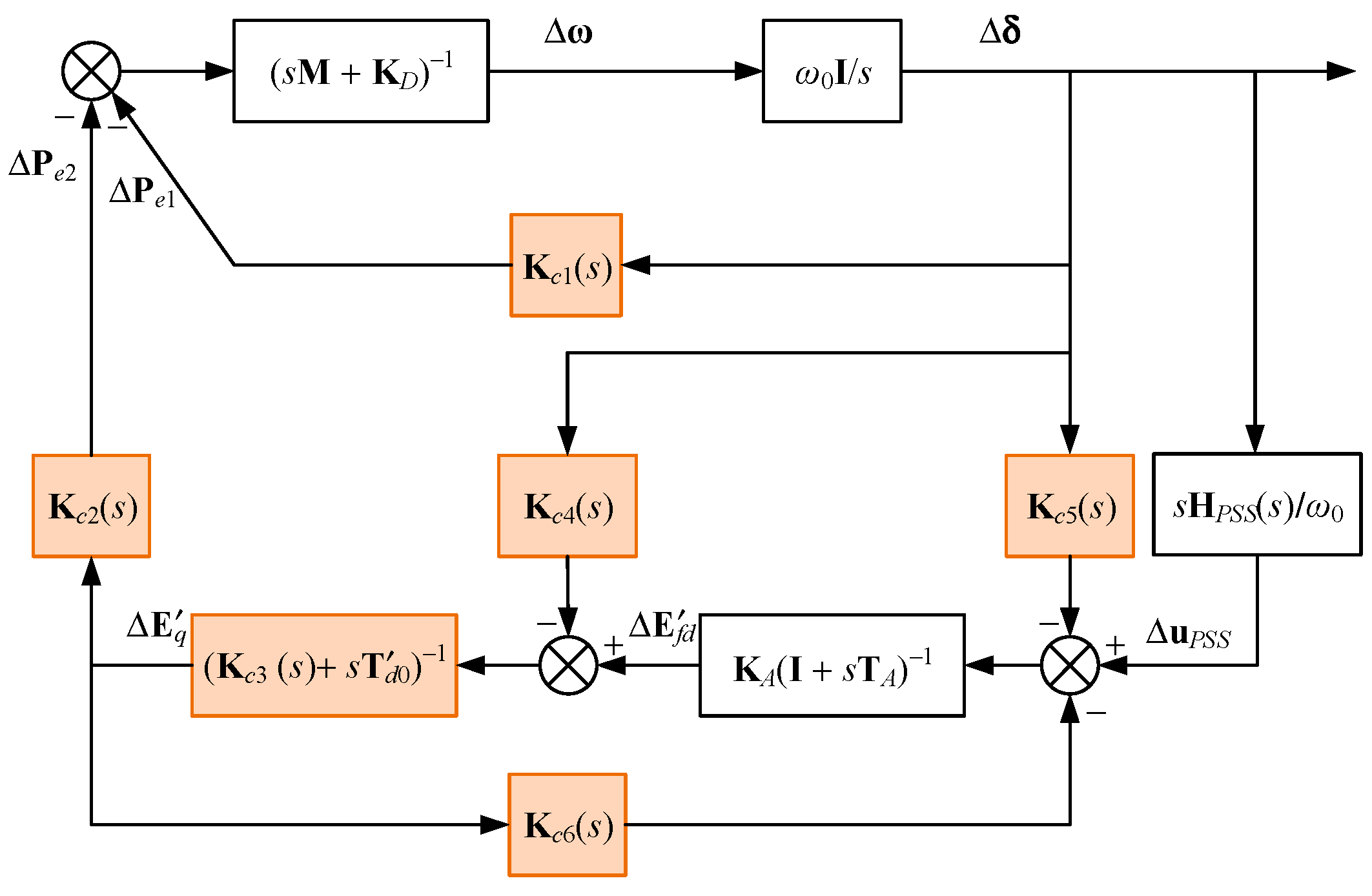
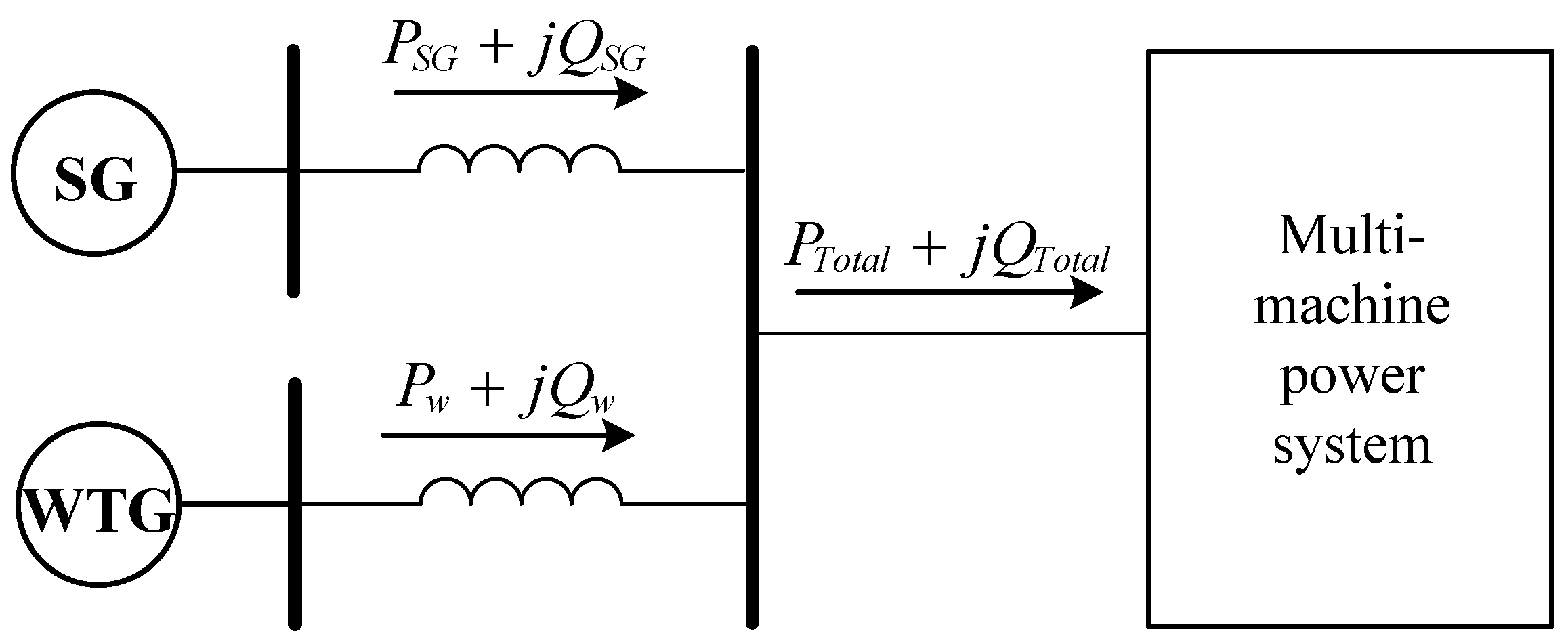
In the Heffron–Phillips model (Figure 1), let us regard the rotor loop (sM + KD)−1 as the feedforward loop, and take the rest of the blocks as the feedback loop; this leads to a compact representation of the rotor-loop Heffron–Phillips model, as depicted in Figure 2.

Figure 1.
Heffron–Phillips model with WTG.
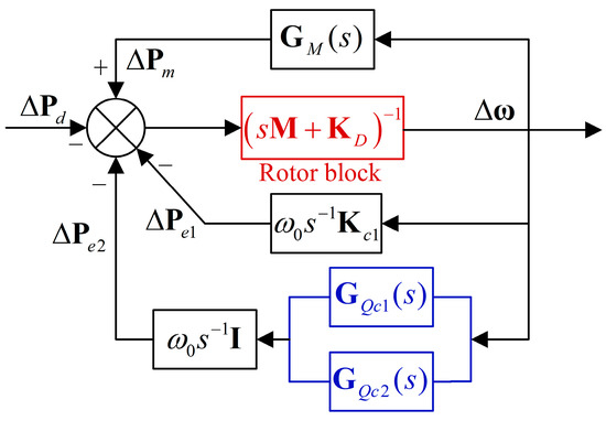
Figure 2.
Block diagram of the Heffron–Phillips model with WTG.
In the figure, GQc1(s) represents the transfer function of the excitation system after wind power integration, while GQc2(s) denotes the transfer function of the additional excitation control (PSS). Their expressions are given as follows:
In addition, the loop transfer function matrix of the complete system is obtained as outlined below:
It is apparent that the above loop transfer matrix plays a key role in determining the overall stability of the system.
2.2. Minimum Characteristic Locus Method Using Similarity Matrix
Substituting into the expression of , one obtains the following:
where M and KD are diagonal matrices, thus
Substitute Equation (14) into Equation (13), the following is obtained:
To proceed the analysis, let us define
In general matrix, Kc1 is diagonalizable; therefore, the following eigen-decomposition holds:
where is a diagonal element of the eigenvalues; and represents the corresponding eigenvector. Notice the following:
It follows that
where
The stability margin becomes
The above stability indicator can be used to study the impact of the DFIG on low-frequency oscillations very conveniently; however, it is less robust when the changes in system parameters are relatively large. The next two sections will describe an enhanced method that proves to be more robust, providing high-fidelity stability assessment.
3. Power System Stabilizer Design Using Inverse Characteristic Locus Method
Substituting into the expression of , one obtains the following:
To understand the impact of controller loops on system stability, a transformation is required. First notice that
Substitute the above result into Equation (22) to obtain the following:
For convenience, introduce the following variable
where LKc1(jω), LKD(jω), and LGQc1(jω) represent, respectively, the open-loop frequency response matrix of synchronous machines, damping terms, and excitation systems; and LGM(jω) and LGQC2(jω) represent the frequency response matrix corresponding to speed-governor and power-system stabilizers.
Let us perform the following similarity transformation:
where the entries of the diagonal matrix consist of the eigenvalues of the first four terms in Equation (26); and U is the corresponding eigenvector.
Introduce the following similarity matrix:
It is apparent that the eigenvalues of the matrix coincide with those of the frequency response matrix L(jω). Since, as in [17],
It is, therefore, clear that the eigenvalues of the inverse matrix can be viewed as a stability indicator.
Notice the following:
Let
where
Substituting Equation (31) into Equation (30), one obtains the following:
Further, let
where
Substituting Equation (33) into Equation (32), the following is obtained:
Now suppose there exist m synchronous machines, and further, let hPSS,i(jω) represent the frequency response of the i-th machine, the following expression is obtained:
For convenience, let E(jω) represent the matrix and express the eigenvector matrix U as follows:
It follows
Following the standard Woodbury formula
Equation (36) can be simplified as outlined below:
Introduce
It follows that
The above formula can be explored to conveniently design power system stabilizers. Specifically, one should choose the phase of stabilizers at a given frequency so that the characteristic locus is farther away from the −1 point in the complex plane, see Section 5 for a design example.
4. Stability Analysis Using Inverse Characteristic Locus Method
In this section, the effect of the grid integration of wind turbines on the open-loop transfer function matrix of the system is investigated by replacing the synchronous machine output with a WTG (Figure 3).
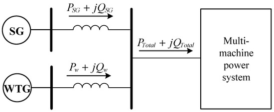
Figure 3.
Schematic diagram of WTG replacing synchronous machine.
Assume that the oscillation frequencies before and after replacement are and , respectively. Then, the loop transfer function matrices before and after the replacement can be represented as outlined below:
Then, rewrite as follows:
In which
From the above equation, it can be seen that the change in the open-loop transfer function matrix due to the replacement of the synchronous machine output by the WTG can be decomposed into the change in the open-loop transfer function matrix of the three loops, ∆LKc1, ∆LGQc1, and ∆LGQc2. According to Equation (9), it can be seen that Kc1(s)–Kc6(s) can be decomposed into two parts, and then, ∆LKc1, ∆LGQc1, and ∆LGQc2 can also be decomposed into two parts affected by the dynamic change in the WTG and the synchronous machine.
For ∆LKc1, the following expression is obtained:
The situation is similar for ∆LGQc1 and ∆LGQc2. Therefore, based on Equation (18), Equation (41) can be rewritten as follows:
According to the Woodbury formula:
The expression for the inverse matrix of the similarity matrix SM is derived as follows:
Since the inverse matrix of the similar matrix is highly diagonally dominant, the stability margin of the system can be better approximated by using the inverse of its diagonal element furthest from the −1 point. According to the above equation, the effect of the change in turbine dynamics on the stability margin and the effect of the change in system tidal current on the stability margin after increasing the turbine output can be obtained.
5. Case Studies
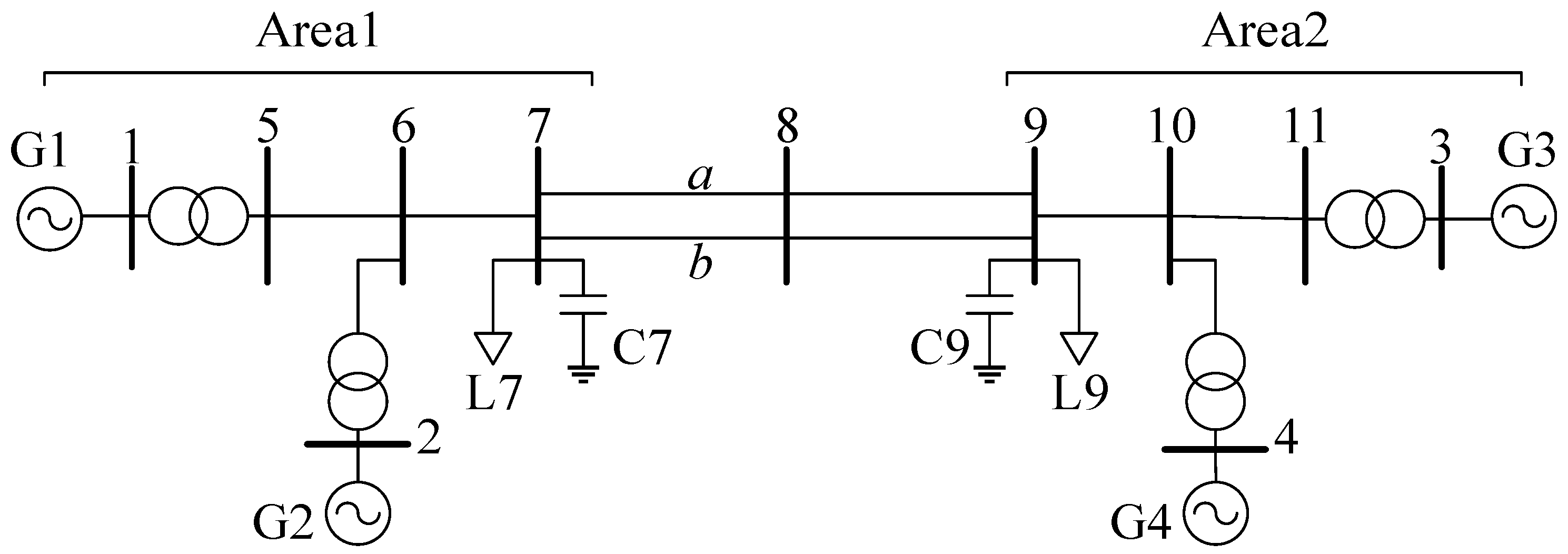
In this section, the inverse characteristic locus method presented in the previous sections is used to study the stability of the familiar 4-machine-2-area system [18] (Figure 4 below).

Figure 4.
Four-machine-two-area system.
5.1. Power System Stabilizer Design
In this example, based on Equation (38), four stabilizers were designed; the compensation angles and corresponding eigenvalue results are summarized in Table 1.

Table 1.
The impact of PSS on area mode.
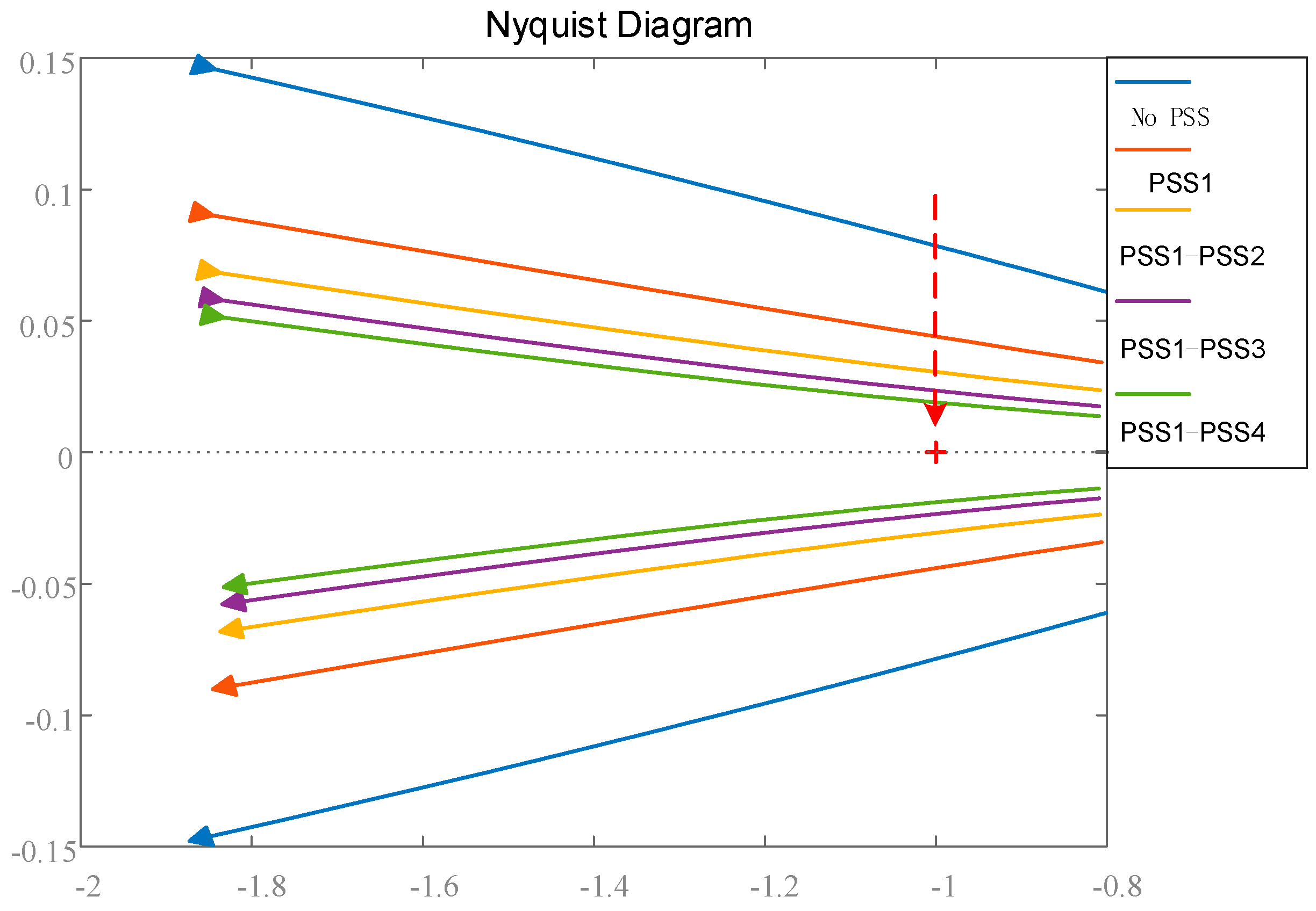
As can be seen from the table, the installation of stabilizers helps improve the damping levels. Figure 5 below further illustrates the characteristic locus of the system after the installation of stabilizers. The figure shows that as more and more stabilizers are installed, the locus gradually approaches the −1 point in the complex plane, indicating the improvement in the stability margin.
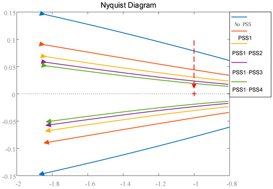
Figure 5.
Characteristic locus after the installation of stabilizers.
5.2. The Impact of the DFIG on Low-Frequency Oscillations
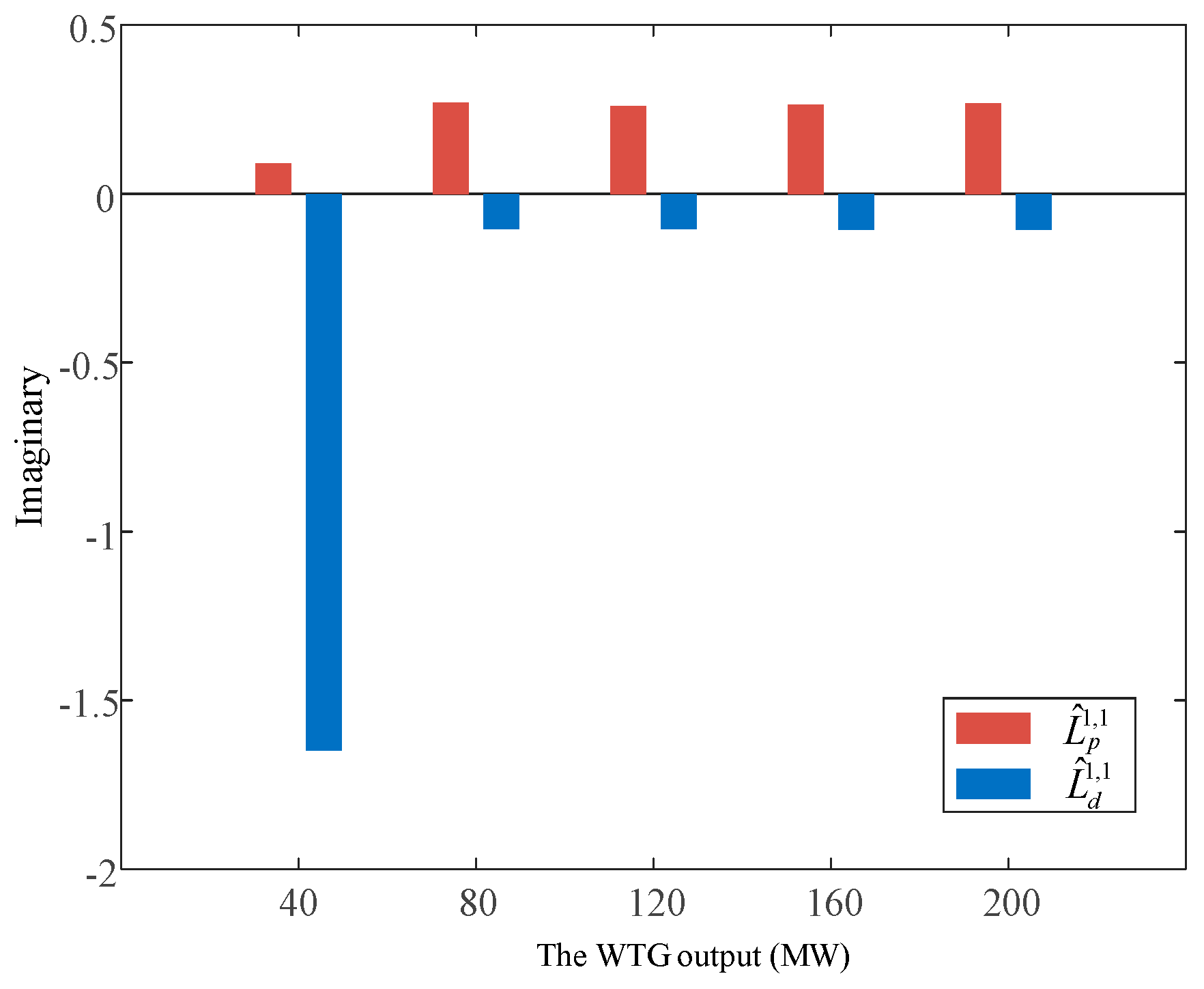
In this sub-section, the effects of and after the turbines are connected to the system are reported, and the errors in the stability margins obtained by the characteristic locus method and the inverse characteristic locus method are also compared. The turbine model used here is a DFIG. Firstly, the wind turbine is connected to bus 6, and the wind turbine output is increased to 40 MW, 80 MW, 120 MW, 160 MW, and 200 MW sequentially, while the load with the same power is added at bus 7 to dissipate the wind turbine output.
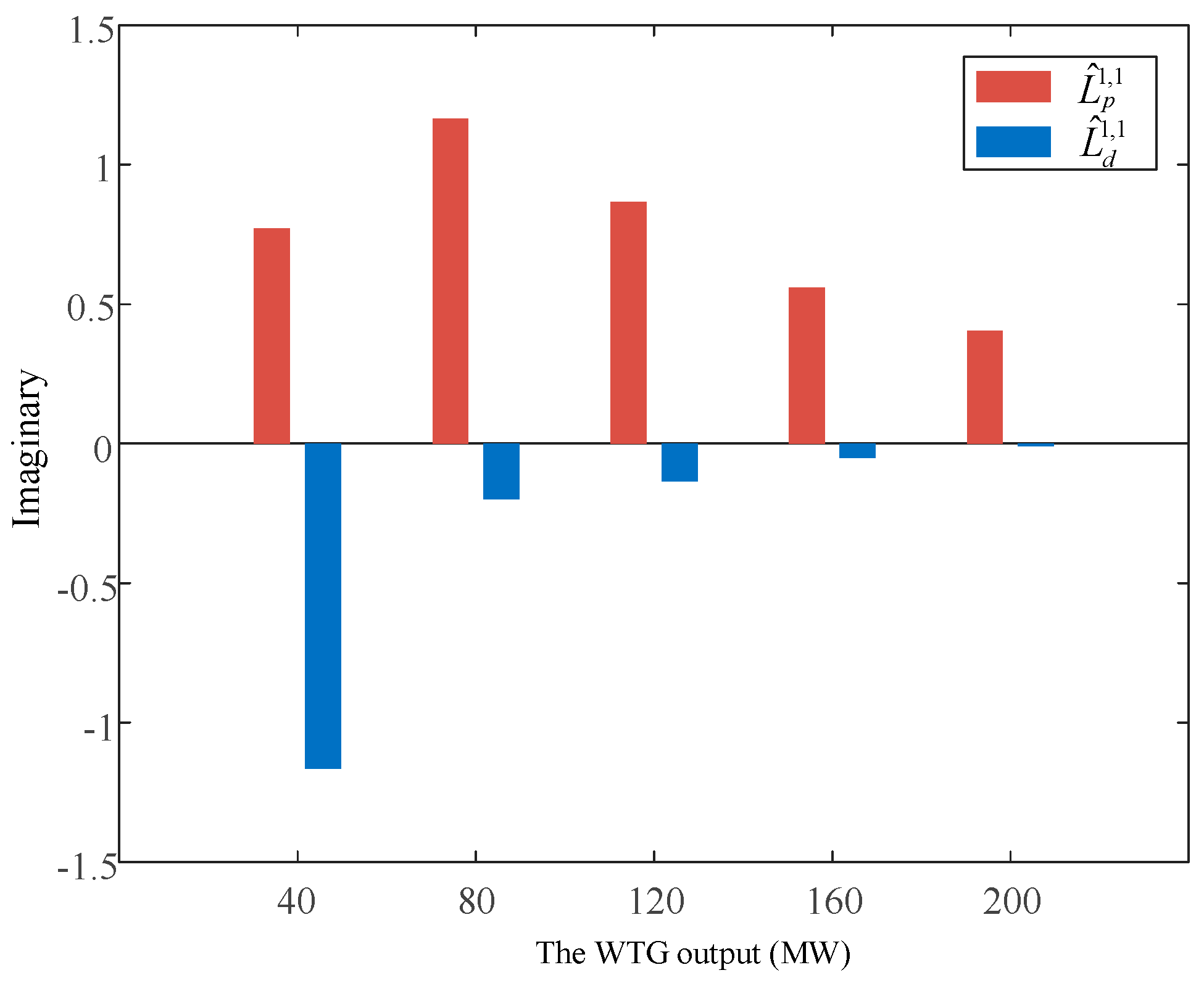
Figure 6 shows the effect of and on the stability margin when the WTG output is increased at delivery bus 6 (load L7 is increased at bus 7). It can be seen from the figure that during the process of increasing the WTG output, the influence of the system trend change on the stability margin is always negative, while the influence of the change in the WTG dynamics on the stability margin is always positive, and when the WTG is connected to the system for the first time, makes the stability margin of the system have a large increase, and after that, the influence of is obviously smaller and basically remains unchanged. In contrast, has the smallest effect on stability when the turbine is first connected to the system, after which the effect increases and remains within a stable range. Overall, except for the initial connection of the turbine to the system, the impact on the stability margin caused by changes in system currents is greater than that caused by changes in turbine dynamics.
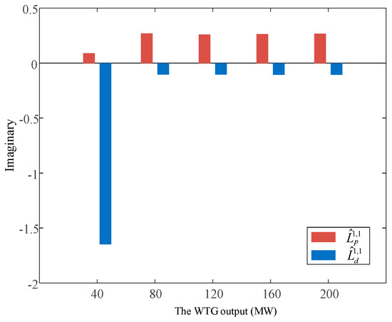
Figure 6.
Effect of and on the stability margin (L7).
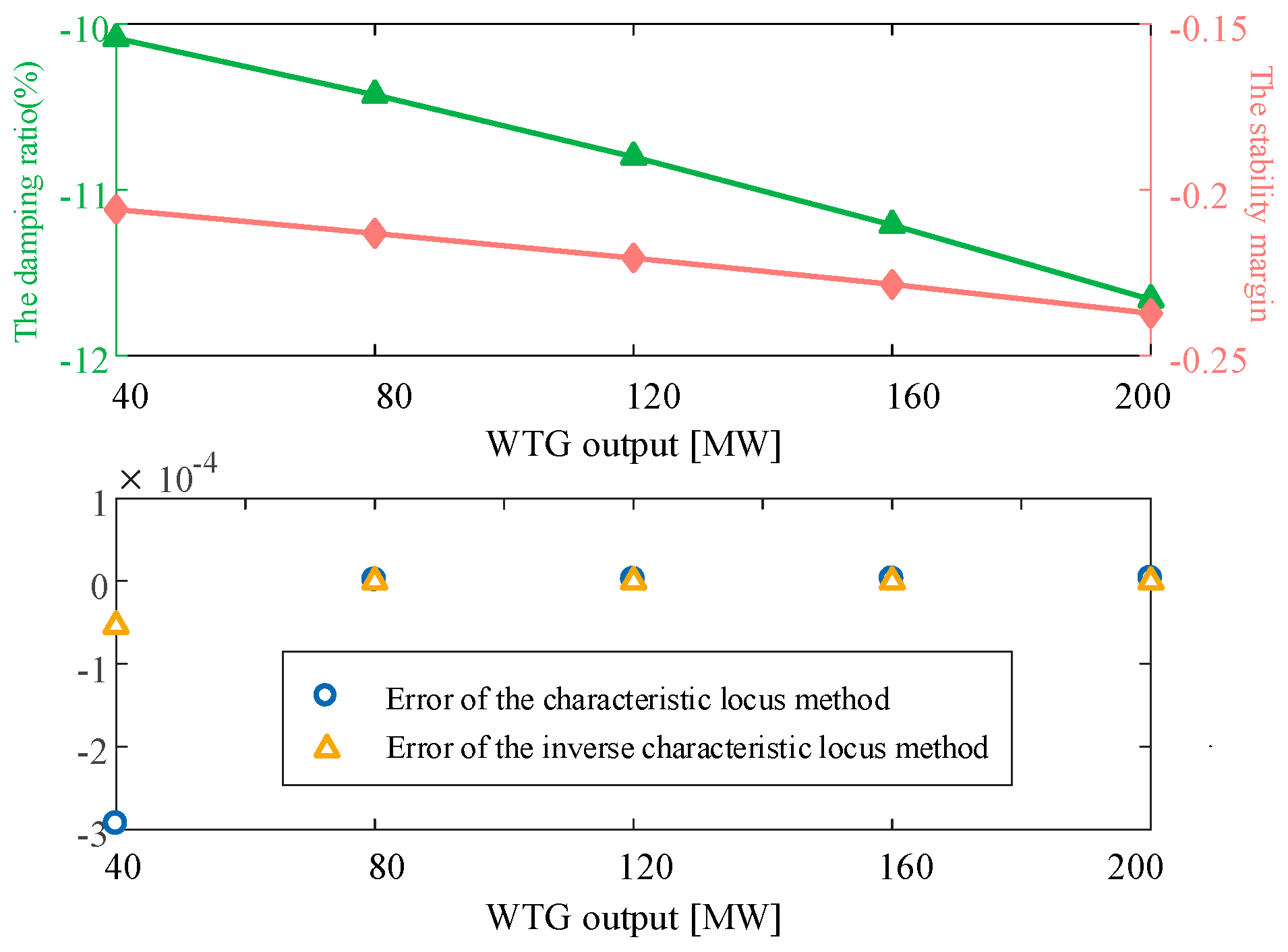
Figure 7 compares the trends of the damping ratio and stability margin of the system when the WTG output force is gradually increased. It can be seen that they have the same trend, i.e., the stability of the system is gradually weakened with the increase in WTG output. In addition, the error of the approximation of the stability margin obtained by the characteristic locus method and the inverse characteristic locus method is also compared with that of the WTG power change, and it was found that the error of the stability margin obtained by the two methods in the initial connection of the WTG to the system is relatively large but the error of the inverse characteristic locus method is smaller than that of the characteristic locus method, and after that, it is basically the same as the accurate value. It is worth noting that the errors of both methods are on the order of minus 4 of 10, which is on a low level.
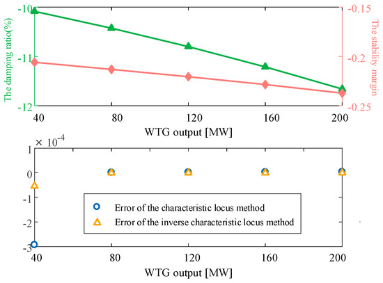
Figure 7.
Comparison of the damping ratio and stability margin of the system (L7).
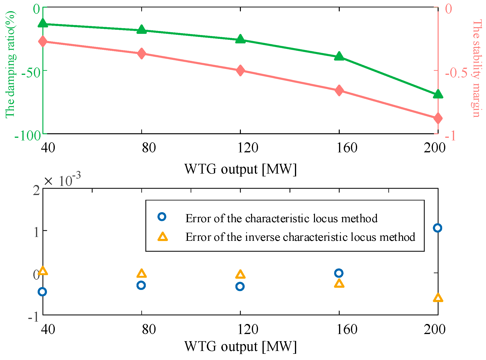
The effects of and on the stability margin when the WTG output at bus 6 is increased, accompanied by a corresponding increase in load L9 at bus 9, are shown in Figure 7. Similar to Figure 5, the effects of are all negative and the effects of are all positive, and except for the first connection of the turbine, the effects of are much larger than the effects of . The positive effects of and on the stabilization margin are shown in Figure 8. The difference is that, with the gradual increase in the WTG’s output, the positive influence of is obviously weakened, while the effect of shows a trend of first increasing and then decreasing.
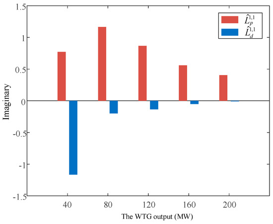
Figure 8.
Effect of and on the stability margin (L9).
From Figure 8, it can be seen that the stability of the system is gradually weakened with the increase in the WTG’s output, and it can be seen from Figure 9 that dominates the trend of weakening stability. It can also be seen that the stability margins obtained by both the characteristic locus method and the inverse characteristic locus method maintain a high degree of accuracy but the accuracy of the stability margins obtained by the inverse characteristic locus method is higher compared to the characteristic locus method.
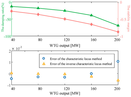
Figure 9.
Comparison of the damping ratio and stability margin of the system (L9).
6. Conclusions
This paper proposes an inverse characteristic locus method to analyze the impact of wind power integration on low-frequency oscillations in power systems. The proposed method is applied to a standard 4-machine 11-bus test system, providing quantitative insights into the stability margin variations under different wind turbine placements and operating conditions. The results indicate that when the wind turbine is connected at the sending end of the system and its output increases, the system’s stability margin decreases. Conversely, when the turbine is connected at the receiving end and its output increases, the stability margin improves. Furthermore, in systems with long-distance transmission lines, if the turbine’s output is primarily consumed by loads at the sending end, the stability margin improves. However, if the output is mainly dissipated by loads at the receiving end, the stability margin deteriorates. Additionally, the analysis reveals that when the wind turbine is integrated into the system with increasing output, the impact of system power flow changes on stability is consistently more significant than the effect of turbine dynamic behavior. These findings provide valuable insights for planning and control strategies in power systems with high wind power penetration.
Author Contributions
Conceptualization, H.X. and D.G.; methodology, H.X. and D.G.; formal analysis, P.S.; writing—original draft preparation, D.G.; writing—review and editing, C.W.; supervision, P.S. and Y.W.; project administration, X.W. and C.F.; funding acquisition, J.B. and B.C. All authors have read and agreed to the published version of the manuscript.
Funding
This research was funded by the Science and Technology Project of the State Grid Sichuan Electric Power Company (52199723000P).
Data Availability Statement
The original contributions presented in this study are included in the article. Further inquiries can be directed to the corresponding author.
Conflicts of Interest
Authors Peng Shi, Yongcan Wang, Xi Wang, Chengwei Fan, Jiayu Bai and Baorui Chen were employed by State Grid Sichuan Electric Power Research Institute. The remaining authors declare that the research was conducted in the absence of any commercial or financial relationships that could be construed as a potential conflict of interest. The authors declare that this study received funding from the State Grid Sichuan Electric Power Company. The funder had the following involvement with this study: supervision, project administration, and funding acquisition.
References
- Bu, S.Q.; Zhang, X.; Zhu, J.B.; Liu, X. Comparison analysis on damping mechanisms of power systems with induction generator based wind power generation. Int. J. Electr. Power Energy Syst. 2018, 97, 250–261. [Google Scholar] [CrossRef]
- Du, W.; Bi, J.; Cao, J.; Wang, H.F. A Method to Examine the Impact of Grid Connection of the DFIGs on Power System Electromechanical Oscillation Modes. IEEE Trans. Power Syst. 2016, 31, 3775–3784. [Google Scholar] [CrossRef]
- Zhang, H.; Zhou, Y.; He, W.; Hu, J.; Huang, W.; Li, W.; Zhai, S. Mechanism Analysis of Low-Frequency Oscillation Caused by VSG from the Perspective of Vector Motion. Processes 2024, 12, 2303. [Google Scholar] [CrossRef]
- Pai, M.A.; Gupta, D.P.S.; Padiyar, K.R. Small Signal Analysis of Power Systems; Apha Science: London, UK, 2004. [Google Scholar]
- Wang, H.; Du, W. Analysis and Damping Control of Power System Low-Frequency Oscillations; Springer Science + Business Media: New York, NY, USA, 2016. [Google Scholar]
- Demello, F.P.; Concordia, C. Concepts of Synchronous Machine Stability as Affected by Excitation Control. IEEE Trans. Power Appar. Syst. 1969, 88, 316–329. [Google Scholar] [CrossRef]
- Larsen, E.V.; Swann, D.A. Applying Power System Stabilizers. Part I: General Concepts. IEEE Power Eng. Rev. 1981, 1, 62–63. [Google Scholar] [CrossRef]
- Pagola, F.L.; Perez-Arriaga, I.J.; Verghese, G.C. On sensitivities, residues and participations: Applications to oscillatory stability analysis and control. IEEE Trans. Power Syst. 1989, 4, 278–285. [Google Scholar] [CrossRef]
- Crusca, F.; Aldeen, M. Multivariable frequency-domain techniques for the systematic design of stabilizers for large-scale power systems. IEEE Trans. Power Syst. 1991, 6, 1133–1139. [Google Scholar] [CrossRef]
- Li, S.; Wang, Y.; Zhang, H. Design method of multivariable PI controller for turboprop engine based on equivalent transfer function. Chin. J. Aeronaut. 2024, 37, 237–260. [Google Scholar] [CrossRef]
- Shi, P.; Jiang, C.; Gan, D.; Xin, H.; Jia, L.; Gao, X.; Xu, Y.; Xie, H. New Value Set Approach for Robust Stability of Power Systems With Wind Power Penetration. IEEE Trans. Sustain. Energy 2019, 10, 811–821. [Google Scholar] [CrossRef]
- Zhou, J.; Shi, P.; Gan, D.; Xu, Y.; Xin, H.; Jiang, C.; Xie, H.; Wu, T. Large-Scale Power System Robust Stability Analysis Based on Value Set Approach. IEEE Trans. Power Syst. 2017, 32, 4012–4023. [Google Scholar] [CrossRef]
- Zhang, Q.; Luo, J.; Zhang, D.; Yang, M.; Xu, H.; Gan, D. A Method to Identify the Impact of Wind Turbine Generator on Low-Frequency Oscillations. IEEE Trans. Power Syst. 2024, 39, 5699–5711. [Google Scholar] [CrossRef]
- Xu, H.; Gan, D.; Zhang, Q.; Huang, W.; Zeng, P.; Huang, R. A Small-Signal Stability Analysis Method Based on Minimum Characteristic Locus and Its Application in Controller Parameter Tuning. IEEE Trans. Power Syst. 2024, 39, 3798–3810. [Google Scholar] [CrossRef]
- Zhang, Q.; Gan, D.; Huang, W.; Xu, H.; Wu, S.; Huang, R.; Zeng, P. A Characteristic Loci Method for Power Systems Small-signal Stability Analysis and Control Design. Int. J. Electr. Power Energy Syst. 2023, 148, 482–488. [Google Scholar] [CrossRef]
- Heffron, W.G.; Phillips, R.A. Effect of a Modern Amplidyne Voltage Regulator on Underexcited Operation of Large Turbine Generators. Trans. Am. Inst. Electr. Engineers. Part III Power Appar. Syst. 1952, 71, 692–697. [Google Scholar] [CrossRef]
- Wang, G.; Xin, H.; Gan, D.; Li, N. A Probability-one Homotopy Method for Stabilizer Parameter Tuning. IEEE Trans. Power Syst. 2013, 28, 4624–4633. [Google Scholar] [CrossRef]
- Klein, M.; Rogers, G.J.; Moorty, S.; Kundur, P. Analytical investigation of factors influencing power system stabilizers performance. IEEE Trans. Energy Convers. 1992, 7, 382–390. [Google Scholar] [CrossRef]

Disclaimer/Publisher’s Note: The statements, opinions and data contained in all publications are solely those of the individual author(s) and contributor(s) and not of MDPI and/or the editor(s). MDPI and/or the editor(s) disclaim responsibility for any injury to people or property resulting from any ideas, methods, instructions or products referred to in the content. |
© 2025 by the authors. Licensee MDPI, Basel, Switzerland. This article is an open access article distributed under the terms and conditions of the Creative Commons Attribution (CC BY) license (https://creativecommons.org/licenses/by/4.0/).