Evaluating Waste Heat Potential for Fifth Generation District Heating and Cooling (5GDHC): Analysis Across 26 Building Types and Recovery Strategies

Abstract

Efficient cooling and heat recovery systems are becoming increasingly critical in large-scale commercial and industrial facilities, especially with the rising demand for sustainable energy solutions. Traditional air-conditioning and refrigeration systems often dissipate significant amounts of waste heat, which remains underutilized. This study addresses the challenge of harnessing low-potential waste heat from such systems to support fifth-generation district heating and cooling (5GDHC) networks, particularly in moderate-temperate regions like Flanders, Belgium. To evaluate the technical and economic feasibility of waste heat recovery, a methodology is developed that integrates established performance metrics—such as the energy efficiency ratio (EER), power usage effectiveness (PUE), and specific cooling demand (kW/t)—with capital (CapEx) and operational expenditure (OpEx) assessments. Empirical correlations, including regression analysis based on manufacturer data and operational case studies, are used to estimate equipment sizing and system performance across three operational modes. The study includes detailed modeling of data centers, cold storage facilities, and large supermarkets, taking into account climatic conditions, load factors, and thermal capacities. Results indicate that average cooling loads typically reach 58% of peak demand, with seasonal coefficient of performance (SCOP) values ranging from 6.1 to a maximum of 10.3. Waste heat recovery potential varies significantly across building types, with conversion rates from 33% to 68%, averaging at 59%. In data centers using water-to-water heat pumps, energy production reaches 10.1 GWh/year in heat pump mode and 8.6 GWh/year in heat exchanger mode. Despite variations in system complexity and building characteristics, OpEx and CapEx values converge closely (within 2.5%), demonstrating a well-balanced configuration. Simulations also confirm that large buildings operating above a 55% capacity factor provide the most favorable conditions for integrating waste heat into 5GDHC systems. In conclusion, the proposed approach enables the scalable and efficient integration of low-grade waste heat into district energy networks. While climatic and technical constraints exist, especially concerning temperature thresholds and equipment design, the results show strong potential for energy savings up to 40% in well-optimized systems. This highlights the viability of retrofitting large-scale cooling systems for dual-purpose operation, offering both environmental and economic benefits.

1. Introduction

Decarbonizing heating and cooling in the built environment remains a pressing challenge, especially in densely populated urban areas, business parks, and university campuses, where district energy solutions are typically beneficial. A lot of models have been created to simulate a district heating (DH) system in energy analysis software and to determine the waste recovery potentials according to different heat recovery methods. These district heating systems enable the utilization of waste heat and operate at ultra-low network temperatures, belonging to the concept of fifth generation district heating and cooling (5GDHC) [1,2,3]. Such systems offer an innovative approach by integrating decentralized, low-temperature thermal networks that operate bidirectionally and enable energy sharing between prosumers. These systems leverage waste heat recovery, thermal storage, and smart control to balance supply and demand while reducing overall energy consumption and emissions. However, typically, a performance comparison of the proposed configurations, which include cooling units (e.g., absorption chillers [4]), is performed with no regard for the source of waste heat. For instance, in [5], the outdoor natural cold resource is used with the help of a refrigerant loop, while heat recovery is achieved by connecting the main condenser in parallel. The second condenser directly supplies warm air to the staff office to satisfy heating demands.

In the transition from conventional heating systems to more efficient district solutions, the role of building envelope performance becomes crucial. Reference [6] on 4GDH emphasizes the thermal inertia and storage potential within building envelopes, highlighting that buildings themselves can act as dynamic components of the heating system through heat accumulation and delayed dissipation. This principle is particularly relevant when considering building-specific characteristics such as insulation and glazing, which directly affect both the cooling demand and the ability to recover and reuse waste heat. In this study, we account for envelope performance in the evaluation of building types (e.g., data centers, supermarkets, cold storage), aligning with the 4GDH perspective that buildings must be considered active thermal elements rather than passive recipients.

The spatial and infrastructural configuration of 5GDHC systems is as critical as their thermodynamic performance. The approach presented in [7], using a top-down GIS-driven methodology, provides valuable insight into optimizing network layouts by leveraging urban form, density, and energy demand distribution. Although this study focuses on the micro-level—variations in cooling profiles and waste heat utilization by building type—it complements our previous macro-level approach by enriching the database with detailed thermal load and waste heat profiles for 26 different prosumer types. Integrating such granular data into GIS-based planning tools could enhance the realism and efficiency of large-scale 5GDHC network design, enabling a more precise match between supply and demand nodes.

Hu et al. [8] suggest using a condenser of the absorption chiller to utilize waste heat. It is then used to regenerate a desiccant solution to achieve latent air cooling. Since the authors also incorporate solar collectors, the heat capacity of cold air significantly increases the seasonal coefficient of performance (SCOP). The system size (required for cooling under the same cooling energy consumption) is potentially considerably decreased. Compared to the utilization concept presented here, waste heat cannot be used for injecting into a 5GDHC network. In [9], when the indoor temperature setpoint increases by 2 °C during the intermittent demand period, the supply temperature of fresh air is still set at 18 °C and is used to cover the indoor cooling load. This concept is mostly applicable to air handler units of office buildings, and thus cannot be used for any type of building presented here. The reason is that fresh air is typically supplied due to sanitary reasons rather than covering the space cooling load. Another difference is the temperature of injected air, which is fixed at 18 °C, according to the constant enthalpy of the indoor air design condition. Reference [9] refers to a dry-bulb temperature of 24 °C and relative humidity of 55%, which might not match the type of building or cooling system, or might not be in line with local regulations.

Zhang et al. [4] suggest a novel dual-evaporation–temperature combined-effect absorption chiller for air-conditioning applications. The difference is that they suggest producing chilled water at two different temperatures (about 7 and 16 °C), with a COP of approximately 1.1, by the deep utilization of a waste heat source at 100–120 °C. The problem is this temperature level is generally beneficial for power generation rather than covering heating and cooling demands with the help of a 5GDHC system. Keskin et al. [10] report that the computer room air handler-based waste heat utilization method was able to recover approximately 860 kW of heat from the 1200 kW reference data center’s electrical consumption with the standard 18 °C server air supply. In addition to reporting temperatures and configurations, as Keskin et al. [10] did, we study waste heat recovery potential under different building types, cooling technologies, and outdoor temperatures. To compare, in [11], an indicator is power usage effectiveness (PUE): when this is low, most of the energy consumed by the DC is used for computing, which suggests a higher-efficiency cooling system. In [12], a similar modeling assumption is presented: a linear trend between coolant temperature and waste heat extraction efficiency.

To the best of the authors’ knowledge, there have been no attempts to study a set of potential prosumers able to improve the flexibility of the energy supply in a 5GDHC system. The research problem is then not reporting various operating characteristics, such as the coolant temperatures, flow rates, and performance indicators, for various building types with similar geometrical characteristics that are located in the same region. The aim of the paper is to study operational and capital costs, seasonal COP, and energy generation for reasonable cooling capacities. However, the main research question is related to the effect of building type on the amount of waste heat available.

While 5GDHC concepts have been explored in various case studies, most focus on system-level configurations, temperature ranges, or singular building types such as residential or office buildings. However, there remains limited insight into how building-specific cooling demands and thermal profiles—particularly across a diverse range of commercial and industrial sectors—impact waste heat reuse potential. This variation is crucial for optimizing 5GDHC system design, especially when sizing thermal storage, selecting equipment, or forecasting seasonal operational modes.

In this context, this study presents a comprehensive techno-economic assessment of potential waste heat sources across 26 different building types, including data centers, supermarkets, ice rinks, industrial facilities, and wastewater treatment plants. By integrating performance modeling with building-specific parameters (e.g., floor area, internal cooling load, envelope characteristics, equipment specifications), the study evaluates both cooling demand profiles and excess heat recovery potential under multiple operational modes.

This study is among the first to systematically quantify and compare the cooling load and waste heat reuse characteristics across such a broad spectrum of building types in the context of 5GDHC systems. The findings aim to support energy planners and engineers in identifying high-value prosumers, improving network flexibility, and maximizing the utilization of locally available excess heat.

2. Materials and Methods

Specific cooling demand in [kW/t] units is typically used for larger commercial and industrial air-conditioning, heat pump, and refrigeration systems [13]:

kW/ton = P_c/E_r,

(1)

where

• P_c is energy consumption [kW];
• E_r is the amount of heat removed converted into tons of coolant, since the temperature of chilled water is fixed.

An example is that if a chiller’s efficiency is rated at 1 kW/t, then the COP is 3.5 and the EER is 12. Then, 1 kW/ton = 12/EER. Energy efficiency ratios (EERs) are assumed according to [14]; these are 3.0 for the chiller with a water-cooled condenser—or the dry cooler, 3.9 for the chiller with an air-cooled condenser, and 4.9 for the chiller with a water-cooled condenser—or the cooling tower. The method uses the usual metric of capital expenditure (CapEx, Figure 1) to assess the feasibility of waste heat utilization, which can be expressed in the regression form (Equation (2)).

CapEx = 103.46⋅P + 5491.9,

(2)

where P is the installed capacity [kW].

PUE is defined as follows [11]:

PUE = P_Cooling + P_Electrical + P_IT,

(3)

where

• P_Cooling is the power demand of the cooling system;
• P_Electrical are the distribution losses and auxiliary energy consumption;
• P_IT is the energy demand for the Information and Communication Technology (ICT) processes.

The ability of a chiller to remove excessive heat correlates with the chiller’s surface area (Figure 2).

The chiller is defined as a packaged device including a compressor, solenoid valves, condensers, a reservoir, a refrigerant pump, an electronic expansion valve, and an evaporator [5]. To assess the efficiency of the waste heat extraction η_WH, the following expression, based on data from the Aquasar application in Zurich (Switzerland) [12], was used:

η_WH = 0.005993·T₁ + 1.18,

(4)

where T₁ is the coolant temperature [°C].

According to the literature, in a supermarket building, only 10% of heat is absorbed from food, while displays operating with high temperature gradients with indoor air and constantly opened doors are responsible for the rest of the useful energy use [15,16]. In large buildings (e.g., cold storage), around 30% of energy is dissipated due to the poor distribution of cold with the help of air [17]. The highest energy saving rate of 50% is achieved for a data center with no intermittent operation, for which a chiller-based system is designed for the cooling of server racks only [18,19]. For any building type, an average cooling demand is defined according to the Air-Conditioning, Heating and Refrigeration Institute (AHRI) standard [20]

0.01 (100% load) + 0.42 (75% load) + 0.45(50% load) + 0.12 (25% load),

(5)

NPLV, or Non-Standard Part Load Value, is an efficiency rating for chillers that measures their performance under various operating conditions, particularly at part load, which is a more realistic scenario than full-load operation. It provides a weighted average efficiency, considering the chiller’s operating hours at different loads and the impact of ambient conditions on the entering water temperature. Then, for an average chiller,

NPLV = 14.6 EER (kW/TR = 0.822),

(6)

This method relies on the waste heat category and source assumptions, as well as qualitative and quantitative data acquisition methods.

Table 1. Methods of data acquisition for waste heat sources and technical overview.

Parameter	How It Is Measured	Equipment Used	Preliminary Evaluation	Uncertainty and Consistency
Internal Cooling Load (kW or TR)	Calculated via building energy simulation, sub-metering, or from equipment specs and operating hours	Energy meters (BTU meters)—Chiller logs/SCADA systems—Building Management Systems (BMS)	Assigned according to the category of waste heat source (Table 2, Category and Source columns), see the Cooling Capacity column	±5–10% depending on measurement method. Metered data are more accurate than estimates. Inconsistent in older facilities without BMS
Total Floor Area/Volume (m2/m3)	Direct measurement from architectural drawings or on-site survey	CAD/BIM models—Laser scanners or manual tape measurement	Derived from GIS databases (e.g., OpenStreetMap and Google Maps)	±1–2% for documented buildings. Reliable and consistent unless the documentation is outdated
Space Usage	Based on the facility function and occupancy profile. Documented in operational or zoning data	Site inspections—Facility zoning records—Occupancy schedules	Assigned according to the category of waste heat source (Table 2, Category and Source columns), see Space Usage column	Qualitative, but generally consistent. May vary slightly due to mixed-use areas
Envelope Performance	Estimated from construction documents or thermal imaging; assessed with U-values and infiltration rates	IR cameras—Blower door tests—Construction specs (R/U-values)	Assigned according to the category of waste heat source (Table 2, Category and Source columns), see Envelope Performance column	±10–20% if undocumented. Consistency varies greatly, especially in retrofitted or poorly documented buildings
Cooling Equipment Type/Model	Taken from technical datasheets, on-site audits, or maintenance logs	Nameplates—Maintenance records—Equipment tags/photos	Assigned according to the category of waste heat source (Table 2, Category and Source columns)	±0% if tagged correctly, but errors occur if undocumented or equipment has been modified
Flow Rates	Measured with flow meters in HVAC loops or inferred from pump curves	Ultrasonic/electromagnetic flow meters—Pressure sensors + pump specs	Assigned according to the category of waste heat source (Table 2, Category and Source columns) and total floor area/volume (Table 2)	±2–10%, depending on calibration. Consistency depends on flow meter maintenance and placement
ΔT (Temperature Difference)	Directly measured between supply and return lines	Thermocouples/RTDs—BMS temperature sensors	Assigned according to the category of waste heat source (Table 3, Waste Heat Temp. column) and 5GDHC network temperatures	±1–2 °C, more reliable in digital systems. Potential errors if sensors are miscalibrated or poorly located
Compressor and Refrigerant Types	From equipment specs, labels, or maintenance documentation	Equipment datasheets—On-site inspection	Assigned according to the category of waste heat source (Table 3, Equipment Specification column)	High confidence if the documentation is recent. Inconsistent in older or modified plants
Waste Heat Potential	Derived from cooling load + ΔT + run hours. Estimated or calculated	Engineering assessment tools—SCADA or BMS trend logs	Assigned according to the category of waste heat source (Table 3, Waste Heat Temp. column)	Uncertainty is high (±15–30%) if based on assumptions. Medium if monitored data are available

summarizes how the main parameters are measured, the equipment used, and the uncertainty and consistency of the data.

For each entry, typical waste heat temperature ranges, cooling capacity, and heat recovery feasibility are described.

Table 2. Waste heat source technical overview.

#	Category	Source	Cooling Capacity	Total Floor Area/Volume	Space Usage	Envelope Performance
N/A	N/A	N/A	kW/MW	m2/m3	N/A	N/A
1	Data Center	Air/Water	200–400 kW	1000–3000 m2	Data center (hot aisle)	Moderate (R-7 walls, R-4 roof)
2		Water/Water	200–400 kW	2000–5000 m2	Data center	Good (raised floor, R-10 walls)
3		In-row Cooling	300–600 kW	1000–2000 m2	High-density racks	High-performance, R-10+
4		In-rack Cooling	600–1200 kW	800–1500 m2	Blade racks	Very high, controlled environment
5		Rear Door HE	200–400 kW	1000–3000 m2	Server room	Good (pressurized room)
6		Cold Plates	300–800 kW	600–1200 m2	GPU/CPU racks	Very high
7	Supermarket	1-comp-r (single compressor)	200–600 kW	500–1500 m2	Retail + cold aisles	Basic, single-glazed front
8		Multiplex	1–10 MW	1000–3000 m2	Grocery retail	Basic-medium
9		50% indirect cooling	500–1500 kW	1200–2500 m2	Supermarket	Medium
10		100% indirect	80–200 kW	1500–3000 m2	Supermarket	Medium-good
11	Cold Storage	Chilled	200–400 kW	800–1500 m3	Logistics warehouse	High (insulated, R-30 walls)
12		Deep-freeze	1–5 MW	500–1000 m3	Frozen storage	Very high (foam walls, <R-35)
13	Ice Skating	Industrial (ammonia)	~500–1000 kW equiv.	1800–3000 m2	Recreation/sports	Poor to moderate
14		Decentralized (Rxxx refrigerant)	200–400 kW	1200–2500 m2	Sports rink	Variable
15		Decentralized (ammonia)	200–400 kW	1000–2000 m2	Sports/recreation	Variable
16		Industrial (Rxxx refrigerant)	300–600 kW	1800–3000 m2	Recreation	Medium
17	Indoor Ski	-	600–1200 kW	10,000–20,000 m3	Sports and leisure	Very high (enclosed, foam-insulated)
18	Plastic Industry	Blow Molding	200–400 kW	2000–5000 m2	Industrial hall	Poor to medium
19		Plastic Extrusion	300–800 kW	3000–6000 m2	Industrial hall	Poor to medium
20		Injection Molding	200–600 kW	2000–5000 m2	Industrial	Medium
21	Heavy Industry	Chemical	1–10 MW	10,000–30,000 m2	Industrial	N/A (process buildings)
22	Food Industry	-	500–1500 kW	3000–8000 m2	Processing	Good (hygienic panels)
23	Winery	-	80–200 kW	1500–3000 m2	Fermentation halls	Moderate (brick/concrete)
24	Brewery	-	200–400 kW	2000–4000 m2	Brew hall + cold storage	Moderate
25	Biomass	Boiler Plant	1–5 MW	N/A	Thermal plant	N/A
26	WWTP (Wastewater)	Effluent	~500–1000 kW	Variable	Utility/process	Moderate

includes the engineering and facility-specific parameters.

Table 3. Extended waste heat source dataset: key assumptions and parameters.

#	Category	Source	Waste Heat Temp.	Cooling Type	Equipment Specification	Conclusion
	N/A	N/A	°C	N/A	N/A	N/A
1	Data Center	Air/Water	28–35	CRAH + chiller	CRAH + air-cooled chiller, ~60–80 L/s, ΔT ≈ 7 °C, Scroll/Rotary, R410A	Moderate temp., medium-grade heat
2		Water/Water	30–40	Rear door HE	Rear-door HE + chilled water loop, ~100 L/s, ΔT ≈ 10 °C, Screw, R134a	Higher-grade heat; ideal for 5GDHC
3		In-row Cooling	25–30	Localized air cooling	In-row DX or glycol-cooled units, ΔT ≈ 6 °C, Scroll/Rotary, R410A	Short loop, fast cycling
4		In-rack Cooling	30–38	Liquid cooling	Direct liquid (cold plate), ~15–25 L/s, ΔT ≈ 8 °C, Micro-compressor, R1234yf	Higher temp; compact HE potential
5		Rear Door HE	32–45	Water loop	Water loop, rear door HE, ~60–80 L/s, ΔT ≈ 10 °C, Scroll/Screw, R513A	High-grade recovery; scalable
6		Cold Plates	40–50	Direct-to-chip	Cold plate + liquid loop, low flow high ΔT, Pump-driven, R1233zd	Highest quality niche adoption
7	Supermarket	1-comp-r (single compressor)	20–28	Air cooled	R404A DX units, ~40 L/s, ΔT ≈ 6 °C, Reciprocating, R404A	Low-temp recovery, limited use
8		Multiplex	25–35	Centralized rack	Central rack with remote condensers, ~80 L/s, R407F or R448A	Better recovery potential
9		50% indirect cooling	28–34	Glycol loop	Glycol loop, centralized rack, ΔT ≈ 6–8 °C, Scroll, R448A	Compatible with 5GDHC
10		100% indirect	30–36	Fully decoupled	Full secondary loop, ΔT ≈ 8 °C, Semi-hermetic, R744 (CO2)	Efficient for HE integration
11	Cold Storage	Chilled	15–25	DX system	R717 (ammonia) or CO2, Recip/Screw, ~60 L/s, ΔT ≈ 5 °C	Low-grade; depends on usage
12		Deep-freeze	5–15	NH3 or CO2	Screw compressor, cascade system, R744 or R717	Very low-grade; not ideal
13	Ice Skating	Industrial (ammonia)	20–28	Ammonia loop	Flooded NH3 system, ΔT ≈ 4–5 °C, Open-screw	Low-grade, but steady
14		Decentralized (Rxxx refrigerant)	22–30	DX split systems	DX system, Scroll/Semi-hermetic, R407C	Common in older rinks
15		Decentralized (ammonia)	20–28	NH3	Reciprocating NH3 units, ΔT ≈ 5 °C	Similar performance
16		Industrial (Rxxx refrigerant)	20–28	Packaged chillers	Chiller plant + secondary glycol, R448A or R404A	Often retrofitted
17	Indoor Ski	-	10–20	Mixed ammonia/CO2	NH3/CO2 cascade, ΔT ≈ 4 °C, Twin-screw, flooded	Very low-grade, hard to reuse
18	Plastic Industry	Blow Molding	35–60	Process cooling	Chiller + tower loop, ΔT ≈ 6–10 °C, Scroll/Screw, R407C	Good match for heat pumps
19		Plastic Extrusion	40–70	Closed-loop glycol	Glycol loop, ΔT ≈ 8–10 °C, Screw, R134a	High-grade waste heat
20		Injection Molding	30–55	Mixed circuits	Process chiller + loop, ΔT ≈ 6 °C, Scroll/Recip, R410A	Compatible with heat pump recovery
21	Heavy Industry	Chemical Sector	60–100 °C	Heat exchangers	Steam exchangers, Shell and Tube HE, Open-screw, R717/R245fa	Industrial-grade recovery
22	Food Industry	-	35–60 °C	Steam or hot water	Process chillers + glycol loops, ΔT ≈ 8 °C, Scroll/Screw	Often uses internal recovery
23	Winery	-	30–45 °C	Chillers	Chiller + fan coils, R410A, ΔT ≈ 5–7 °C	Seasonal operation limits use
24	Brewery	-	45–65 °C	Steam/CO2	Chiller plant + jacket cooling, ΔT ≈ 6 °C, R404A	Good integration potential
25	Biomass Plant	-	60–90 °C	Steam/water loop	Steam turbines + ORC, ΔT ≈ 15–25 °C, Water/Steam, R245fa	Excellent recovery profile
26	WWTP (Wastewater)	-	20–30 °C	Heat exchangers	Sludge digestion + effluent heat exchanger, ΔT ≈ 5 °C	Needs heat pump boost

outlines the assumed technical specifications for each waste heat source in the expanded list.

3. Case Study

This section narrows down the general assumptions listed in Table 2 and Table 3 and exemplifies them with existing buildings in a particular region. A significant advantage compared to the conventional system, with an energy saving potential of up to 40%, is expected when units for waste heat recovery are installed in large buildings. Although with the increase in outdoor temperature the energy demand diminishes rapidly and even becomes negative, the climatic conditions of the Flanders region (Belgium) are assumed to be acceptable for hosting a 5GDHC system, enabling extensive heat use in winter and large potential for waste heat utilization due to hot summers.

3.1. Example of Cold Storage

In Figure 3, a large building used for cold storage, located in Zellik (Flanders, Belgium), is presented as the first example.

The evaluation is based on the operating hours of 8760 h, an electricity price of 0.11 EUR/kWh, an average outdoor temperature of 10.47 °C, and chilled water temperatures set to 12/6 °C.

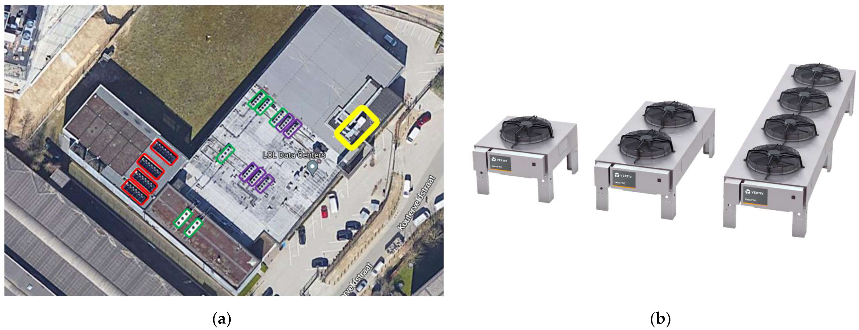
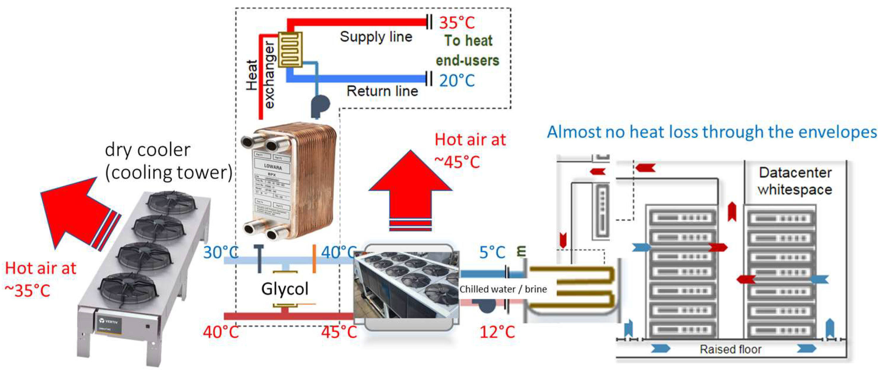
3.2. Example of a Data Center

Another eminent source of constantly produced low-potential waste heat is data centers. Figure 4 shows the main elements of the reference configuration of an air-cooled data center: a server room, a pumping station, a plate exchanger, a chiller, and a cooling tower (or a dry cooler).

In Figure 4, the heat exchanger splits indoor (containing water) and outdoor (containing water–glycol solution) conduits. A cooling tower (or a dry cooler) is responsible for removing excess heat, which is claimed by the network operator (e.g., in the late summer, when seasonal thermal energy storage (TES) is already full). The reference configuration of any other source of waste heat is assumed to be similar. Figure 5 shows how the suggested configuration might be scaled for different numbers of floors.

Excluding industrial units, data centers are typically the largest producers of low-potential waste heat. The evaporator and electronic expansion valve are typically placed in a data center room (next to the server rack), while condensers and other parts are placed outdoors, e.g., on the top of the staff office room. Figure 6 shows a photo of this integrated system of free cooling and heat recovery.

3.3. Example of a Supermarket Building

If a supermarket building is considered a source of waste heat [22], the application zone where the novel system is superior noticeably narrows to large buildings only, as shown in Figure 7.

4. Results and Discussion

This section first describes the operation in two modes, using a data center as an example, and then compares the amount of waste heat potentially recovered under the assumptions listed in Table 2 and Table 3. It is a top-down approach, which does not delve into the details of the particular HVAC systems but compares their potential based on type only.

4.1. Example of a Data Center

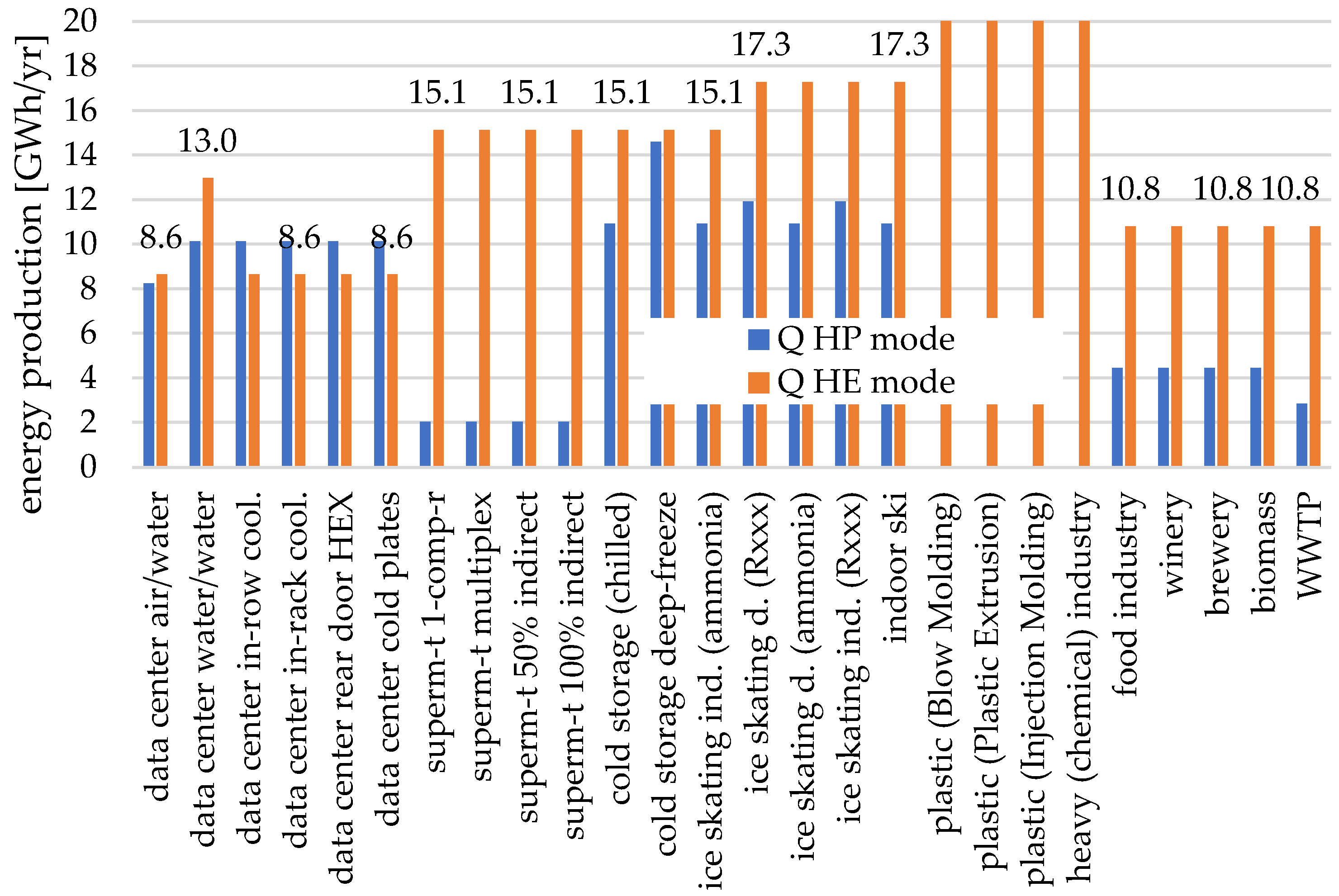
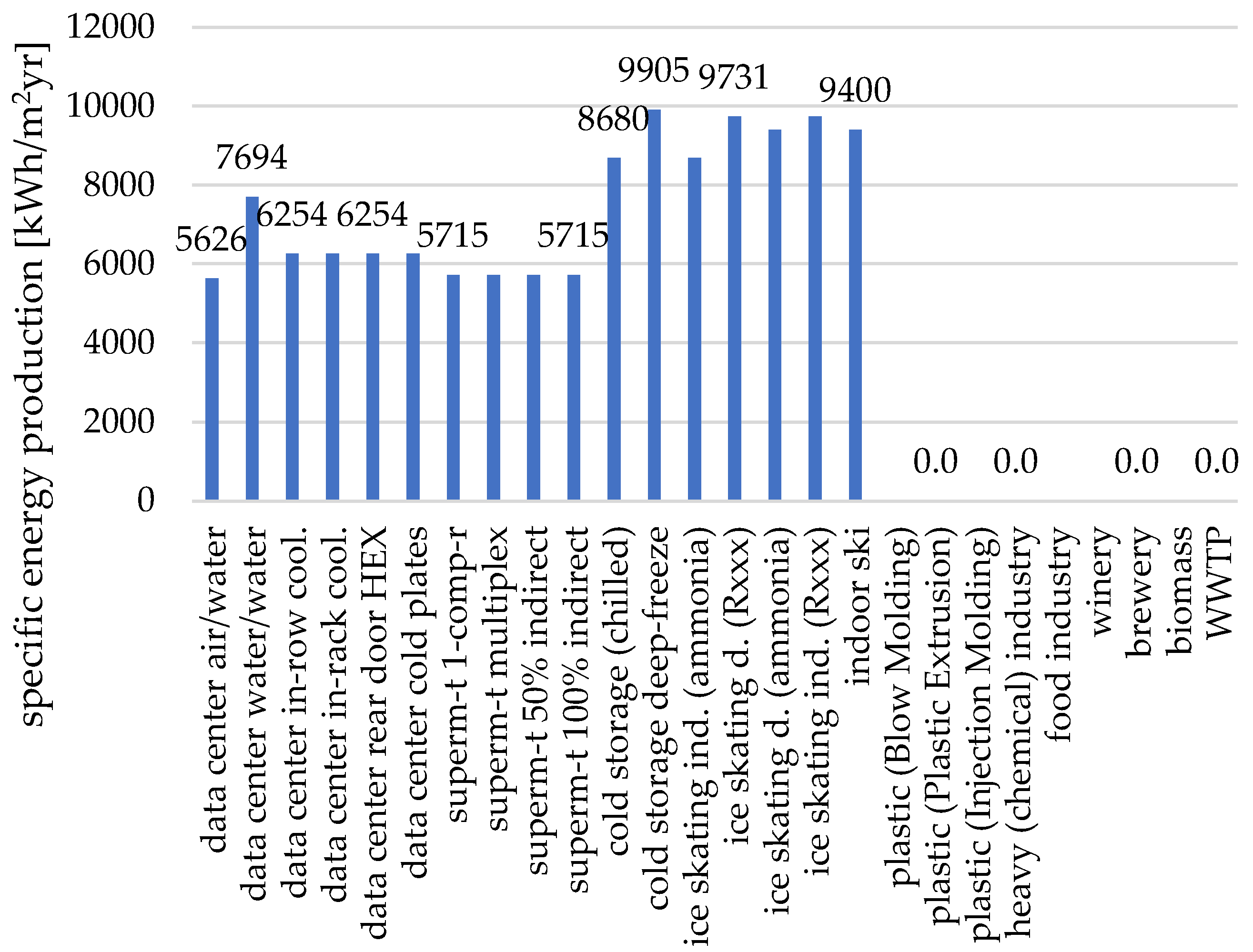
This example serves to demonstrate operating in two modes: summer (heat exchanger) and winter (booster heat pump). However, this is not the case for all the sources of waste heat. According to Table 3, some of them require a heat exchanger only or cannot operate without a booster heat pump due to the low potential of waste heat.

According to Equation (5), the average cooling demand is as follows:

0.01(1) + 0.42(0.75) + 0.45(0.5) + 0.12(0.25) = 0.58 of the peak demand

That means that multiplying peak cooling capacity by 0.58 provides a rough estimate of the average chiller load = (324.8 TR) = 188.4 TR [20]. In June-August, the temperature of waste heat is higher than the network temperature, so only a heat exchanger is required (Figure 8).

For different water and air temperatures, as long as the indoor setpoints stay constant, both the flow rate in the primary circuit and the surrounding air-conditioned environment would maintain thermal equilibrium. HE is the least expensive component, so the cooling load almost does not affect CapEx. At the same time, OpEx tends to considerably increase for the lower temperature of waste heat and lower COP (as presented below).

The distribution of energy production also depends on the number of operating hours when the temperature of waste heat is higher than the network temperature. The difference is typically negative when the outdoor temperature is relatively high. Another factor for southern locations is the air humidity. However, that is not relevant for Belgian climate conditions. Large electricity demand in a heat exchanger mode indicates that the proposed system may inject much higher flow rates in the network and operate as a heat source similar to a boiler of a conventional system (Figure 9).

For a data center, the type of cooling system is defined as either air or liquid cooling. The latter includes in-row and in-rack cooling, rear door heat exchangers, and cold plates, all having the same generation in heat pump (HP) and heat exchanger (HE) modes of 10.1 and 8.6 GWh/yr due to the same air/water ratios and operational temperatures. On the other hand, the lower temperature of cooling water decreases COP, leading to a lower energy generation in the heat pump mode, which is relevant for supermarkets with chilled water at 12/6 °C, an indoor temperature of 18 °C, and a relative humidity of 50%. For larger buildings, the water temperature might be higher. In data centers, the inlet air temperature of the server and the inlet water temperature are assumed to be higher at 30 °C and 40 °C, respectively. In the HP mode, the effects of the availability of heat recovery and waste heat ratio on W_elec are less significant than expected. An example of the temperature distribution when operating in the first mode is presented in Figure 10.

The first task is to ensure the reliable cooling of expensive ICT equipment, and only then to utilize waste heat. No ICT endangering is allowed; therefore, removing chillers or any modernization of the internal cooling conduits is not considered.

4.2. Comparison

As shown in Figure 11, for most of the potential prosumers, OpEx outbalances CapEx and has nearly the same value of 1.32 kEUR/yr for all types of supermarket, which highlights that this component of a 5GDHC system can only feasibly work with a capacity factor above 55%.

Network temperature is restricted to 35 °C in this paper. That means that the water temperature in the supply (warm) line of a 5GDHC network never exceeds 35 degrees Celsius. The chiller power results in lower costs for a higher OpEx because of a lower PLR and a higher COP. The max and min differences between CapEx and OpEx are 2.03% (data center) and 2.50% (deep freeze cold storage), respectively. Despite all the differences between them in terms of influencing mechanisms, this balance indicates that an optimal or nearly optimal configuration of equipment has been achieved. For all these buildings, the number of cooling units depends on the building type only. In real life, this value may drastically vary, while in the given analysis, it is considered reasonable for a building with a surface area of 3000 m² (Figure 12).

According to the simulations, depending on the type of cooling system, between 33% and 68% of the waste heat can be converted to useful heat. In Figure 12, 0 indicates sources of waste heat to which no surface-area-specific values can be applied. However, a 59% heat recovery ratio might be considered as the average and accepted as a mid-case scenario to generate input data for a simulation of a 5GDHC system based on excess heat recovery. Unlike other buildings with a large cooling demand, in a data center, IT power consumption, lighting power, and CRAH fan powers are almost fully converted to heat, although only up to 70% of the heat can be usefully utilized.

However, proper heat exchanger sizing is necessary to ensure chiller cooling and therefore design temperature difference between the supply (typically 5 or 6 °C) and the chilled water returned (typically 11 or 12 °C). Due to the lower temperature difference, compared to heating units, cooling ones typically operate with a higher flow rate and a lower water transport factor, which therefore has less impact on the cooling demand. If the peak-to-base load ratio is high, the COP curve crosses the optimal point related to the highest COP, causing higher energy consumption. As a result, the OpEx component associated with chillers, water pumps, and other auxiliary equipment would increase, shifting the more or less optimal trade-off between OpEx and CapEx obtained by applying a rule of thumb (refer to Figure 11). Eventually, this causes the total costs to increase drastically, while COP drops. To alleviate such an adverse effect, a storage tank for coolant is also installed. After this, a heat pump and a heat exchanger are installed, wherethe latter is the third largest component of CapEx. According to the presented simulations, the max SCOP is 10.3 and the average is 7.4 (Figure 13).

The highest SCOP matches the scenario of installing a water-to-water heat pump in an air-cooled data center (see Figure 10). When studying seasonal variation, these results demonstrate that the waste utilization rate drops substantially with the outdoor temperature decreases, which is expected since almost all the chillers are able to work in a free-cooling mode. This mode typically takes place in winter and can be called the third operational mode, where no waste heat utilization is possible.

To compare, Hnayno et al. [11] discuss data centers only where the cooling system is a combination of air and liquid cooling. For a system that includes rear-door heat exchangers and air/water cooling units, they report a fixed supply water temperature of 27 °C and a return water temperature ranging from 30 to 40 °C. In [9], the variations in temperature and cooling demand on peak load are considered negligible, with total deviations of up to only 2.5%. However, the range of secondary fluid cooling is also narrow in that paper (from 1.0 to 1.3). Song et al. [9] also discuss the differences between types of cooling systems from the point of view of influencing mechanisms. For a cooling system with a chiller, energy consumption is lower for a higher intensity of secondary fluid cooling due to the lower partial load ratio and higher COP.

In the literature, for a data center, the IT power consumption, lighting power, and fan powers of computer room air handlers are typically assumed to be constant and fully converted to heat [23]. If so, up to 100% of the heat could be recovered. However, Keskin et al. [10] report that only between 55% and 90% of the waste heat can be converted to useful heat. In their paper, a 72% heat recovery ratio was input as a mid-case scenario for calculating a data center’s excess heat recovery system. All these values are higher compared to those obtained in the present paper. Song et al. [9] also emphasize specific features of cooling units such as a higher chiller capacity, lower temperature difference between supply and return temperatures, a higher flow rate, and a lower water transport factor, which, on the other hand, has less impact on the cooling load. Another similar aspect is studying the effect of the share of secondary fluid cooling. The authors conclude that, when this is more than 1.4, the COP profile can cross the highest point, causing the COP of the chiller to gradually decrease. An effect is that the power of chillers, water pumps, and other auxiliary equipment also increases, resulting in higher peak loads. These two effects are the same as those discussed in the present paper, which corroborates the results and obtained profiles.

Here, we implement a simplified approach, dividing a year period into three operational modes based on the outdoor temperature. In [4], the primary focus is to study the operation of a cooling system under changing external conditions. For instance, for the period when outdoor temperature is extremely high (above 35 °C), the variation range of power and efficiency indicators is more than 100%, while some values become negative, indicating that the proposed system requires much higher heat source flow rates. In [8], operational modes for an absorption chiller mostly depend on the relative humidity. Their results demonstrate that the ability of the coolant to remove excessive heat decreases considerably with relative humidity, which is expected since the total water content has dropped. For instance, to compensate for the lowered water partial pressure under a lower relative humidity, the steady-state salt concentration in the desiccant substantially rises. Variations in the relative humidity lie outside of the scope of the present paper.

When comparing types of cooling systems, insights from at least two papers are relevant. For instance, as mentioned above, Zhang et al. [4] compare novel and conventional systems under hot and humid climates. They report the same correlation between the outdoor and cooling water temperatures. Second, temperatures in an absorber and a condenser also increase up to 40 °C when the outdoor temperature is 35 °C and the humidity is 80%, which is well in line with the upper and lower temperature thresholds we used in these simulations. Third, as shown in [8], for an absorption chiller, the salt concentration in the desiccant has already nearly hit the crystallization limit for CaCl₂, which highlights that this dehumidifier can only feasibly work with RH conditions beyond 55%. This means that, for an absorption chiller, despite the similarities, the threshold condition is the salt concentration in the desiccant rather than the temperature of waste heat.

5. Conclusions

To sum up, the contribution to the pool of knowledge provided by this study is an approach providing a respective comparison of 26 building types based on an energy and technical analysis of cooling systems. The novelty is the assigning of specific values of energy production, concerning the control method of the cooling system and total heat recovery in the form of both water and air, which can be adopted for three modes available over a year. For different buildings, as long as the indoor setpoints stay constant, both the indoor air-conditioned spaces and the outdoor environment maintain thermal balance, and the cooling load is constant until outdoor temperature changes. A shortlist for necessary inputs is suggested; to simplify the process for designers and decision-makers, this is refined to be as short as possible. For the suggested method, six indicators are sufficient: location (e.g., city name to derive proper profile of outdoor temperature), type of building/process (to assess inlet/outlet temperatures), number of chillers, number of dry coolers, their capacity (Equations (5) and (6) can be used to find average) or surface area (the capacity is then found with the help of regression) and type, and building surface area.

The expected output is the indicators revealing whether the suggested 5GDHC network is feasible, such as total CapEx, savings, and payback period. Before any advanced simulations, it is vital to make sure the potential 5GDHC system, which includes suggested buildings, is even promising. The reason for this is the low specific values of energy generation for some types of buildings and cooling systems, which require including only large buildings. Offering higher efficiency and the better integration of renewables, the 5GDHC concept is a step forward in the decarbonization the energy sector.

References

1. Buffa, S.; Cozzini, M.; D’Antoni, M.; Baratieri, M.; Fedrizzi, R. 5th generation district heating and cooling systems: A review of existing cases in Europe. Renew. Sustain. Energy Rev. 2019, 104, 504–522. [Google Scholar] [CrossRef]
2. Reiners, T.; Gross, M.; Altieri, L.; Wagner, H.J.; Bertsch, V. Heat pump efficiency in fifth generation ultra-low temperature district heating networks using a wastewater heat source. Energy 2021, 236, 121318. [Google Scholar] [CrossRef]
3. Wirtz, M.; Heleno, M.; Moreira, A.; Schreiber, T.; Müller, D. 5th generation district heating and cooling network planning: A Dantzig–Wolfe decomposition approach. Energy Convers. Manag. 2023, 276, 116593. [Google Scholar] [CrossRef]
4. Zhang, F.; Yin, Y.; Cao, B.; Wang, Y. Performance analysis of a novel dual-evaporation-temperature combined-effect absorption chiller for temperature and humidity independent control air-conditioning. Energy Convers. Manag. 2022, 273, 116417. [Google Scholar] [CrossRef]
5. Ding, J.; Zhang, H.; Leng, D.; Xu, H.; Tian, C.; Zhai, Z. Experimental investigation and application analysis on an integrated system of free cooling and heat recovery for data centers. Int. J. Refrig. 2022, 136, 142–151. [Google Scholar] [CrossRef]
6. Chicherin, S. Conversion to Fourth-Generation District Heating (4GDH): Heat Accumulation Within Building Envelopes. Energies 2025, 18, 2307. [Google Scholar] [CrossRef]
7. Chicherin, S. Top-down GIS-driven method for configuring the network layout of a 5th generation district heating and cooling (5GDHC) system. Energy 2025, 328, 136639. [Google Scholar] [CrossRef]
8. Hu, T.; Shen, Y.; Kwan, T.H.; Pei, G. Absorption chiller waste heat utilization to the desiccant dehumidifier system for enhanced cooling—Energy and exergy analysis. Energy 2022, 239, 121847. [Google Scholar] [CrossRef]
9. Song, J.; Peng, J.; Cao, J.; Yin, R.; He, Y.; Zou, B.; Zhao, W. Global sensitivity analysis of fan coil air conditioning demand response—A case study of medium-sized office buildings. Appl. Therm. Eng. 2023, 230, 120721. [Google Scholar] [CrossRef]
10. Keskin, I.; Soykan, G. Optimal cost management of the CCHP based data center with district heating and district cooling integration in the presence of different energy tariffs. Energy Convers. Manag. 2022, 254, 115211. [Google Scholar] [CrossRef]
11. Hnayno, M.; Chehade, A.; Klaba, H.; Bauduin, H.; Polidori, G.; Maalouf, C. Performance analysis of new liquid cooling topology and its impact on data centres. Appl. Therm. Eng. 2022, 213, 118733. [Google Scholar] [CrossRef]
12. Ljungdahl, V.; Jradi, M.; Veje, C. A decision support model for waste heat recovery systems design in Data Center and High-Performance Computing clusters utilizing liquid cooling and Phase Change Materials. Appl. Therm. Eng. 2022, 201, 117671. [Google Scholar] [CrossRef]
13. Understanding Chiller Efficiency. Available online: https://www.linkedin.com/pulse/understanding-chiller-efficiency-omair-farooq (accessed on 20 April 2025).
14. Afonicevs, V.; Strauts, U.; Bogdanovs, N.; Lesinskis, A. Evaporative cooling technology efficiency compared to traditional cooling system—Case study. In Proceedings of the 19th International Scientific Conference Engineering for Rural Development, Jelgava, Latvia, Msy 2020; Latvia University of Life Sciences and Technologies; Volume 19, pp. 877–883. [Google Scholar]
15. Retail Energy Reduction Solutions | Hillphoenix AMS Group. Available online: https://www.hillphoenix.com/products/the-ams-group-products/energy-reduction-solutions/ (accessed on 20 April 2025).
16. Energy Savings Tips for Small Businesses: Grocery and Convenience Stores | ENERGY STAR. Available online: https://www.energystar.gov/buildings/resources-audience/small-biz/grocery (accessed on 20 April 2025).
17. Evans, J.A.; Hammond, E.; Gigiel, A.; Fostera, A.; Reinholdt, L.; Fikiin, K.; Zilio, C. Assessment of methods to reduce the energy consumption of food cold stores. Appl. Therm. Eng. 2014, 62, 697–705. [Google Scholar] [CrossRef]
18. Ni, J.; Bai, X. A review of air conditioning energy performance in data centers. Renew. Sustain. Energy Rev. 2017, 67, 625–640. [Google Scholar] [CrossRef]
19. Zhang, Y.; Zhao, Y.; Dai, S.; Nie, B.; Ma, H.; Li, J.; Miao, Q.; Jin, Y.; Tan, L.; Ding, Y. Cooling technologies for data centres and telecommunication base stations—A comprehensive review. J. Clean. Prod. 2022, 334, 130280. [Google Scholar] [CrossRef]
20. Performance Rating of Water-Chilling and Heat Pump Water-Heating Packages Using the Vapor Compression Cycle. AN-SI/AHRI Standard 551/591 (SI) with Addendum 3, 2021. Available online: https://www.ahrinet.org/search-standards/ahri-550590-i-p-and-551591-si-performance-rating-water-chilling-and-heat-pump-water-heating-packages (accessed on 20 April 2025).
21. Google. Zaventem. 2023. Available online: https://maps.google.com/ (accessed on 20 April 2025).
22. Arias, J. Energy Usage in Supermarkets—Modelling and Field Measurements; Trita-REFR NV—2005:45; Energy Technology, School of Industrial Engineering and Management (ITM), KTH: Stockholm, Sweden, 2005. [Google Scholar]
23. Bram, S. ThermischGrid Zellik. Confidential Report; Bram, S.: Brussels, Belgium, 2020; 79p. (In Dutch) [Google Scholar]
Figure 1. Regression curve based on the manufacturer’s data to assess CapEx.
Processes 13 01730 g001
Figure 2. Correlation between horizontal surface area and cooling capacity according to the manufacturers’ data.
Processes 13 01730 g002
Figure 3. Satellite view of cold storage in Zellik, Belgium: (a) one of the reviews supported a first guess on the building type and suggested the indoor temperature, (b) the same building zoomed in with the area of cooling machines outlined (red), (c) the cooling machines further zoomed in (red) enabling recognition of their size and the number of fans. Adopted from [21].
Processes 13 01730 g003
Figure 4. Principal scheme of waste heat utilization layout (building side only—network side is not depicted). Blue arrows indicate energy flows within the supply (cold) and return (warm) lines of a cooling system.
Processes 13 01730 g004
Figure 5. Configuration of the cooling equipment, presenting its applicability for cooling offices and server rooms at the same time. Red arrows—warm lines, blue arrows—cold lines.
Processes 13 01730 g005
Figure 6. Data center in Zaventem (Belgium) (a) with Vertiv© dry coolers (b) installed on its roof. Yellow—1 rooftop unit (ventilation), green—6 technological dry coolers, purple—5 dry coolers for offices, and red—4 free cooling chillers (monoblock). Adopted from [21].
Processes 13 01730 g006
Figure 7. Due to a lack of cooling equipment, only large supermarket buildings are considered: (a) configuration of the suggested 5GDHC network, (b) satellite view of a supermarket on the left-hand side of the picture, and (c) satellite view of a supermarket on the right-hand side of the picture. Adopted from [21]. Supermarket buildings are marked with red (power plant sign), purple circles are network nodes (i.e., consumer buildings), yellow squares are network forks (valve vaults), and blue lines are network edges (piping sections).
Processes 13 01730 g007
Figure 8. Layout of the equipment necessary to transmit heat to the network in the summer (heat exchanger) mode. According to the concept presented in Figure 4, this configuration is able to remove excess heat since the TES capacity is not infinite.
Processes 13 01730 g008
Figure 9. Energy production when using a heat pump (HP mode) and operating a heat exchanger only (HE mode).
Processes 13 01730 g009
Figure 10. Layout of the units necessary for operation in the winter mode: connecting a heat pump to utilize heat from a data center or any other building with waste heat in March-May and September-October.
Processes 13 01730 g010
Figure 11. Distribution of OpEx and CapEx.
Processes 13 01730 g011
Figure 12. Specific energy production for various types of potential prosumers.
Processes 13 01730 g012
Figure 13. SCOP for different building and cooling system types.
Processes 13 01730 g013