Article

Research on the Degradation Model of a Smart Circuit Breaker Based on a Two-Stage Wiener Process

1
Zhejiang Testing & Inspection Institute for Mechanical and Electrical Products Quality Co., Ltd., Hangzhou 310051, China
2
Intelligent Electrical Appliance Test and Inspection Technology Zhejiang Engineering Research Center, Hangzhou 310051, China
3
Key Laboratory of Low Voltage Apparatus Intelligentization and New Energy Application of Zhejiang Province, Hangzhou 310051, China
4
State Key Laboratory of Reliability and Intelligentization of Electrical Equipment, Hebei University of Technology, Tianjin 300130, China
*
Author to whom correspondence should be addressed.
Processes 2025, 13(6), 1719; https://doi.org/10.3390/pr13061719
Submission received: 26 April 2025 / Revised: 21 May 2025 / Accepted: 28 May 2025 / Published: 30 May 2025
(This article belongs to the Special Issue Fault Diagnosis Technology in Machinery Manufacturing)

Abstract

As the global energy transition moves towards the goal of low-carbon sustainability, it is crucial to build a new energy power system. The performance and reliability of Smart Circuit Breakers are the key to ensuring safe operation. The control circuit is the key to the reliability of Smart Circuit Breakers, so studying its performance-degradation process is of great significance. This study centers on the development of a degradation model and the performance-degradation-assessment method for the control circuit of Smart Circuit Breakers and proposes a novel approach for lifetime prediction. Firstly, a test platform is established to collect necessary data for developing a performance-degradation model based on the two-stage Wiener process. According to the theory of maximum likelihood estimation and Schwarz information criterion, the estimation method of model distribution parameters in each degradation stage and the degradation ‘turning point’ method are studied. Then, reliability along with residual life serve as evaluation criteria for analyzing the control circuit’s performance deterioration. Taking the degradation characteristic data into the degradation model, for example, analysis, combined with the Arrhenius empirical formula, the reliability function at room temperature and the curve of the residual life probability density function is obtained. Ultimately, the average service life of the Smart Circuit Breaker control circuit at room temperature is 178,100 h (20.3 years), with a degradation turning point at 155,000 h (17.7 years), providing a basis for the lifetime evaluation of low-voltage circuit breakers.

1. Introduction

A low-voltage circuit breaker is an important protective switch electrical appliance in the power distribution system. According to statistics, over 80% of the electric energy is distributed and used through the switch electrical appliance [1]. In 2023, the market size of China’s circuit breakers will reach 12.427 billion yuan, and its application will cover various fields of the national economy, such as national defense and military, aerospace, transportation, and electric power [2,3]. Advancements in electronic technology have led to low-voltage electrical devices exhibiting an extended service life and enhanced reliability, with only minimal performance degradation over time [4,5]. Therefore, the reliability evaluation of low-voltage electrical appliances, particularly low-voltage circuit breakers, remains a significant challenge in the industry. To rapidly obtain life data and degradation process data for reliability assessments, as well as to identify product defects promptly, accelerated degradation testing is a crucial method widely employed in research [6,7]. SCB (Smart Circuit Breaker, SCB) is a key part of the intelligent power system in modern society [8]. It is an emerging product in the low-voltage circuit breaker industry. Its internal structure is complex and compact. It is mainly composed of traditional contact mechanical systems and intelligent electronic systems. It can replace the traditional manual opening and closing mode to realize remote automatic opening and closing [9].
In the advancement of reliability engineering, modeling approaches based on failure physics and performance degradation have become the leading research focus [10]. Among them, the reliability modeling method based on failure physics mainly explains the specific mechanism of electronic product failure through electronic products’ physical and chemical information factors. It obtains the accurate failure information of products [11]. The reliability modeling method based on performance degradation pays attention to the data information in the evolution process of electronic product degradation failure. It uses the appropriate mathematical and statistical model to effectively fit the degradation trend to evaluate electronic products’ reliability [12]. Among these, degradation refers to the gradual and irreversible deterioration of key performance parameters in the SCB control circuit over time, under long-term operation or accelerated stress conditions. It is typically reflected by the measurable changes in electrical characteristics, indicating internal aging mechanisms and forming the basis for reliability assessments and lifetime prediction [13]. Based on the Weibull distribution model of degradation quantity and finite element analysis method, Liu Junzuo studied the degradation process of air tightness of a certain type of sensor shell [14]. Aiming at the distribution of an unknown degradation quantity and bounded degradation quantity, Li Jiang et al. [15] proposed a semi-parametric degradation model for assessing the reliability of breaker products, significantly enhancing the accuracy and credibility of the evaluation process. Yu Rongbin studied the performance degradation modeling method of photovoltaic modules. Without the pre-subjective assumption of the distribution type, it can also effectively fit the distribution of degradation at each moment [16]. Tuo Yantian studied the two-stage degradation process of products and used two drift functions to establish the degradation model for each stage [17]. Tang Xuri et al. [18] constructed a bidirectional multi-point grey prediction model and proposed the concept of equivalence for different breaking currents. The proposed model improves the prediction accuracy of the remaining life of low-voltage DC circuit breakers used in photovoltaic systems. Yang Nuoming et al. [19] proposed a method for predicting the electrical life of DC circuit breakers based on the characteristics of DC arc interruption. In this method, contact quality is used to represent the electrical life condition. A contact quality degradation curve is obtained through linear interpolation and is used as a training label for the life prediction network. Most of the previously proposed models primarily address a constant-rate decline scenario in electronic systems, focusing only on a single-phase degradation trend. In actual engineering contexts, the complex internal faults inside electronic systems combined with fluctuating environmental influences result in the observable wear-out process often presenting as multiple distinct stages rather than a single phase. Different stages of wear display specific statistical properties, featuring a “change point” where the speed of performance loss in electronics changes [20,21,22]. This study constructed a reliability degradation model using a two-stage Wiener process method. According to the theory of maximum likelihood estimation and Schwarz information criterion, the estimation method of model distribution parameters and the degradation ‘turning point’ method in each degradation stage are studied. The performance degradation assessment of the control circuit is carried out. Through the example analysis, the curve of the reliability function and the residual life probability density function at room temperature is obtained, and the maintenance strategy of the SCB control circuit is studied based on the results.
The main contributions of this paper are as follows:
(1)
An in-depth study was conducted on the related degradation mechanisms, and its key functional modules are identified. Based on feature extraction and trend analysis of experimental data, the control circuit is found to exhibit a clear two-stage degradation pattern.
(2)
A degradation model based on a two-stage Wiener process is developed. By integrating the maximum likelihood estimation, the Schwarz information criterion, and reliability analysis, the turning point of performance degradation is accurately identified.
(3)
The quantile plot method is used to test the normality of degradation increments at different stages, and the reliability function along with the failure probability density function curve is obtained by extrapolating from the experimental data. The average service life of the control circuit under normal temperature conditions is predicted to be 178,100 h (20.3 years), and the turning point of degradation is estimated at 155,000 h (17.7 years).
This paper is structured into four primary sections: examination of the deterioration mechanism within the SCB control system; identification of crucial components; analysis of degradation trends and development of a two-stage Wiener process-based degradation model; extrapolation of experimental data to derive the reliability and failure density functions, and prediction of the average service life and turning point of degradation under normal temperature conditions.

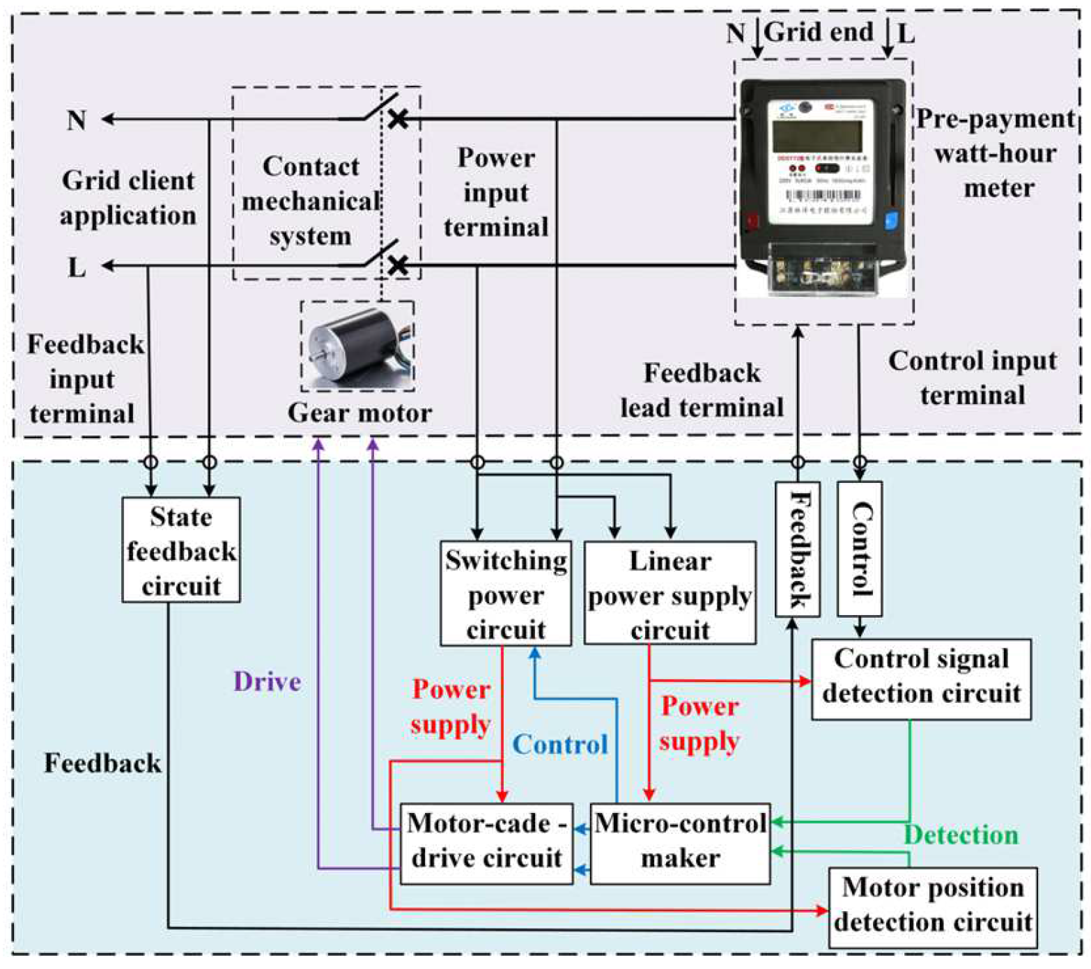
2. Research on the Deterioration Process of the Control System in SCB

2.1. Study on the Functional Mechanism of the Control System

The SCB consists of a contact mechanical system and an intelligent electronic system. The smart electronic setup comprises a control unit and a geared motor. The main function of the control circuit is to receive and judge the external input opening/closing control signal; on the other hand, electric power is transmitted to provide the electric power input for the gear motor. The geared motor transforms the electrical energy supplied by the control unit into mechanical energy to actuate the contact mechanism. The control circuit is the ‘heart’ of the SCB and the key link of the circuit breaker system. Its reliability determines whether the SCB can work reliably and accurately. The principle diagram of the control circuit is shown in Figure 1.
Figure 1 shows that the control unit comprises several operational blocks, including the power module, microcontroller unit, position sensing module, motor driver, control signal acquisition, and feedback for the on/off state. The linear module supplies a constant voltage to the MCU and the signal acquisition subsystem, while the switching section employs low-power design techniques to reduce unnecessary energy consumption for the end user. The control signal acquisition module translates the meter’s status information (e.g., payment in arrears or not) into a direct current (DC) signal, which is then transmitted to the microcontroller for analysis and decision-making. Through the feedback line, the switching status detection circuit conveys connection and disconnection signals of the power system to the energy measurement device. The motor-position-detection circuit is used to detect the motor position and to limit the maximum angle of motor rotation.
Before executing the external control command, the control circuit detects the Hall position and external control signals. Then, it performs different action processes according to the signal state. The complete working logic is shown in Figure 2.
Figure 2 illustrates the automatic control process of the circuit breaker’s opening and closing. After the system is powered on, the motor position is detected by the Hall sensor, and the external control signal is monitored. When a rising edge is detected and the circuit breaker is in the closed state, the start-up power supply drives the motor to reverse to the open position and then locks it. If the circuit breaker is already open, it is directly locked without action. When a falling edge is detected and the circuit breaker is open, the motor drives it to the closed position. If it is already closed, no action is taken. The system remains in a low-power sleep mode when the control signal stays steady. After all operations are completed, the power supply is automatically turned off, and the system enters sleep mode, thereby achieving intelligent control with high efficiency and energy savings.

2.2. Determination of Key Modules

Based on the above theoretical analysis, the following assumption is made: the components have only two states of normal and failure; the system works in the rated input state; the reliability of all components obeys exponential distribution. The exponential distribution has limitations. When assuming that its failure rate is constant, it is not suitable for the description of aging or failure of mechanical components such as bearings and gears.
R ( t ) = e λ t
In the formula, λ refers to the failure occurrence rate; R(t) is the reliability function. According to engineering experience statistics, the time-dependent variation in the failure rates of various components is generally classified into three phases: the initial failure stage, the random malfunction period, and loss failure period. Based on the reliability study of the control unit in the SCB, a mathematical model is established.
λ S = i = 1 n λ i T BF = 1 λ S = 0 R ( t ) d t
In this equation, λS indicates the control circuit’s failure frequency; λi corresponds to the failure frequency of the ith component contained therein; TBF is the average failure-free time. Determine the fault occurrence rate across all constituent elements and functional units, as shown in Figure 3 and Figure 4.
According to the analysis of Figure 3 and Figure 4, electrolytic capacitors and power MOSFETs are the principal components impacting the overall reliability of the circuit system. The main functional elements responsible for system operation are the drive circuits, integrating both the switching power supply and motor drive modules. The above analysis provides a basis for selecting condition-monitoring signals for the accelerated degradation test.

3. Accelerated Degradation Test Design and Characteristic Trend Analysis

3.1. Degradation State Monitoring Signal Selection

The control circuit includes not only device-level degradation monitoring signals, such as capacitance C, equivalent series resistance ESR, etc. It also includes circuit board-level degradation status monitoring signals, such as input voltage signals, output voltage signals, sampling voltage and current signals, and output current signals. Each signal has a coupling redundancy relationship. If these signals are considered for measurement, on the one hand, it will increase the difficulty of data processing and analysis; on the other hand, it will waste test resources. Therefore, by determining the above key modules, combined with the circuit’s topology, the electrical characteristics of the monitoring signal, the difficulty of measurement, and the cost of measurement, the priority of the degradation state monitoring signal is considered. The monitoring signal most representative of the control system’s degradation condition is chosen.
According to the failure statistics of SCB products, most are the failure forms of the closing process [23]. Therefore, the board-level electrical signals related to the control unit during the closing phase of the smart breaker are chosen: motor current, motor terminal voltage, switching power supply voltage, linear power supply voltage, closing and opening control signals, and closing and opening state feedback signals, which are drawn together at the same time, as shown in Figure 5. According to the analysis of the working principle of the control circuit and the characteristics of the electrical signal waveform, the working stages are divided as shown in Table 1.
The critical functional units within the initial segment are identified, considering the circuit’s topology, the monitoring signal’s electrical characteristics, and the measurement’s difficulty and cost. The monitoring signals that can best characterize the control circuit’s performance degradation state are selected as the switching power supply voltage, the motor terminal voltage, and the motor current.

3.2. Accelerated Test Design

Combined with the above-selected degradation state detection signal, accelerated degradation testing is commonly categorized into three distinct forms. As shown in Figure 6, under the premise of a comprehensive consideration of test cost and feasibility, to improve testing efficiency, minimize the number of test samples, and ensure the reliability of data modeling, this study adopts a constant-stress accelerated testing approach.
Several key elements must be considered when developing a scheme for accelerated degradation testing.
(1)
Stress Type and Levels in Accelerated Testing: Temperature is chosen as the sole accelerated stress factor. Typically, a single-stress temperature model requires test data at a minimum of three distinct temperature levels to enable an accurate parameter estimation. The temperature difference between adjacent levels is maintained at no less than 10 °C.
(2)
Determination of Sample Size for Accelerated Testing: Based on prior studies, a standard practice under single-temperature stress conditions is to include five samples per group. This approach minimizes the impact of individual variability on data interpretation and parameter estimation.
(3)
Accelerated Test Duration and Frequency: The test cycle is defined by taking into account changes in performance parameters, the overall testing workload, cost considerations, and the desired quantity of data. An initial inspection interval is established, and subsequent adjustments are made based on observed trends in performance degradation during testing.
The following are the steps of the experiment:
(1)
At 25 °C, the initial values of key condition monitoring signals are recorded as the reference for the samples to evaluate performance degradation.
(2)
The samples are then sequentially subjected to cyclic accelerated aging tests under thermal stress conditions of 105 °C, 95 °C, and 85 °C.
(3)
Each test cycle lasts for 24 h. The process begins with the sample being stabilized at 25 °C for 0.5 h, followed by a temperature increase to the specified stress level over the next 0.5 h. The sample is then operated with one on–off switching cycle lasting 1 h. Afterward, the temperature is reduced back to 25 °C within 0.5 h. Following a 0.5 h hold at this temperature, the sample is removed for a measurement of its condition-monitoring parameters. This process is repeated for the next cycle.
(4)
Until all five samples under each stress fail, the test ends.

3.3. Experimental Data Feature Extraction and Trend Analysis

Due to noise interference in the experimental data, it is necessary to perform denoising before further analysis. Common methods such as wavelet denoising, moving average filtering, and low-pass filtering are applied. The appropriate denoising method is selected based on the signal-to-noise ratio (SNR), which is calculated using the following formula.
S N R = 10 log 1 N i = 1 N n 2 ( i ) 1 N i = 1 N ( n ( i ) s ( i ) ) 2
In the formula, n(i) represents the original degradation state monitoring signal, s(i) denotes the signal after denoising, and N is the total number of signal sampling points. The experimental data were denoised using three different methods, and the signal-to-noise ratio (SNR) was calculated for each. The results are shown in Figure 7.
In general, a higher SNR indicates better signal quality. As shown in Figure 7, wavelet denoising achieves the highest SNR and is therefore selected.
According to the above experimental scheme, the accelerated test is carried out to obtain the sample’s monitoring value under each temperature group. The monitoring data are processed, and the signal-to-noise ratio is calculated and compared. Finally, the wavelet denoising is selected to denoise the data. The extracted feature parameters from the test data include the mean, peak, peak-to-peak, and kurtosis in the time domain; center frequency and standard deviation in the frequency domain; and energy entropy and singular entropy in the wavelet domain. In summary, six feature parameters from the time domain, frequency domain, and wavelet domain can be obtained. Some of these features are highly correlated with performance degradation, while others do not effectively support the evaluation of performance degradation. Moreover, an excessive number of features may impose computational and storage burdens. Therefore, it is necessary to optimize the above characteristic parameters. Therefore, the feature selection method shown in Figure 8 is used to optimize the features.
The feature-selection process shown in Figure 8 is mainly divided into three steps: data acquisition, feature candidate generation, and optimal feature selection. Specifically, the process involves collecting raw data, extracting potential features from the data, and selecting the features that are most relevant to the target task. The core goal is to identify the most critical features from the original data to make the subsequent analysis or modeling more efficient and accurate.
The feature-selection process employs a multi-factor assessment index model to identify the optimal feature parameters. The evaluation considers three dimensions: trend, monotonicity, and robustness. The corresponding formulas are as follows.
T r e ( F , T ) = N i f i t i i f i i t i N i f i 2 ( i f i ) 2 N i t i 2 ( i t i ) 2
Here, F = (f1, f2, , fN) denotes the time series of degradation feature parameters, T = (t1, t2, , tN) represents the corresponding sampling time points, and N is the total number of samples.
M o n ( F ) = i δ ( f i f i 1 ) i δ ( f i 1 f i ) N 1
In the above equation, δ (*) denotes the unit step function.
R o b ( F ) = 1 N i exp ( f i f i ˜ f i )
The comprehensive index formula for multi-dimensional feature evaluation and optimization is derived as follows, based on the above equations.
Z = k 1 T r e ( F , T ) + k 2 M o n ( F ) + k 3 R o b ( F ) s . t . k i > 0 i k i = 1
The test data are brought into the above process for feature selection, and a three-dimensional map of the scoring effect is obtained, as shown in Figure 9.
Figure 9 shows three key feature indices: correlation, monotonicity, and robustness. The candidate feature parameter with the highest score corresponds to the motor terminal voltage’s peak-to-peak amplitude. The score table is shown in Table 2. According to testing and statistical analysis, the failure threshold H for the characteristic parameters is 3 V. The comprehensive score histogram for the corresponding characteristic parameters is shown in Figure 10. By counting the empirical failure date of 15 samples, the failure threshold H of the characteristic parameters can be obtained as 3 V.
Figure 10 shows the comprehensive score of each feature parameter. As shown in the figure, the voltage difference between the highest and lowest points at the motor terminals achieves the highest score, indicating that it is the optimal feature across all dimensions.
The compiled degradation data from samples exposed to various temperature conditions are used to model the characteristic parameter’s degradation trend through least squares fitting. The trend under the three temperature stress levels is consistent, and the fitting trend of 85 °C is shown in Figure 11.
The evolution trend of the degradation characteristics of the five samples is the same. They all experience a relatively stable degradation stage first, pass through the degradation ‘turning point’ at a certain time, and enter the degradation stage with a significantly faster degradation rate. That is, the degradation process of the sample shows a more obvious two-stage nonlinear characteristic. Because the degradation characteristic parameters of the control circuit show obvious two-stage nonlinear characteristics and there is a degradation ‘turning point’, it is difficult to use the traditional linear statistical model to infer. Therefore, this paper proposed a degradation model of the SCB based on the two-stage Wiener process for analysis.

4. Two-Stage Wiener Process Degradation Model

4.1. Degradation Model Construction

Given the research object’s above-mentioned performance-degradation characteristics, a two-stage degradation model should be considered to describe the circuit system’s performance-degradation process. In addition, in the field of reliability engineering, the Wiener process model can describe the inherent randomness of the product degradation path well, and the statistical computational complexity is low, which has a wide range of application research bases. Therefore, this paper uses a two-stage Wiener process model to describe the circuit system’s degradation process. The complete degradation model construction and parameter estimation are based on the flow chart shown in Figure 12.
Define that the first degradation stage obeys the Wiener process X1(t; μ1, σ1), and the second degradation stage obeys the Wiener process X2(t; μ2, σ2), and τ is the time when the turning point of degradation occurs. The control circuit’s two-stage Wiener degradation process model can be expressed as follows.
X ( t ) = X 1 ( t ; μ 1 , σ 1 ) = x 01 + μ 1 t + σ 1 B ( t ) 0 < t τ X 2 ( t ; μ 2 , σ 2 ) = x 02 + μ 2 ( t τ ) + σ 2 B ( t τ )         t > τ
In the expressions above, x01 and x02, are the initial degradation quantities of the first and second degradation stages. μ1 and μ2 are the drift parameters of the first and second degradation stages, respectively, representing the degradation rate of each stage. σ1 and σ2 are the diffusion parameters of the first and second degradation stages. The Wiener degradation process is continuous, and the performance degradation values of the two degradation stages at the degradation turning point are consistent, that is, x1(τ) = x02.

4.2. Parameter Estimation and Turning Point Estimation

A set of m + 1 degradation data with a periodic detection interval Δt = tjtj−1 and degradation increment Δxj = X(tj) – X(tj−1) is obtained from the degradation test. Because the degradation process of the control circuit before and after the degradation turning point is different, the probability density function f(t) of the degradation increment can be expressed in the following two cases:
(1)
When tj < τ, the degradation process is in the first stage. The degradation increment Δxi obeys the inverse Gaussian distribution with drift parameter μ1 and diffusion parameter σ1. The likelihood function of the degradation process increment is as follows:
L 1 ( Δ x i ; μ 1 , σ 1 2 ) = i = 1 k 1 2 π Δ t σ 1 exp ( Δ x i μ 1 Δ t ) 2 2 σ 1 2 Δ t
(2)
When τ < tj−1, the degradation process is in the second stage. The degradation increment Δxi obeys the inverse Gaussian distribution with drift parameter μ2 and diffusion parameter σ2. The likelihood function of the degradation process increment is as follows:
L 2 ( Δ x i ; μ 2 , σ 2 2 ) = i = k + 1 m 1 2 π Δ t σ 2 exp ( Δ x i μ 2 Δ t ) 2 2 σ 2 2 Δ t
The joint likelihood function of the first-stage and second-stage degradation process increments is expressed as follows:
L = i = 1 k 1 2 π Δ t σ 1 exp ( Δ x i μ 1 Δ t ) 2 2 σ 1 2 Δ t i = k + 1 m 1 2 π Δ t σ 2 exp ( Δ x i μ 2 Δ t ) 2 2 σ 2 2 Δ t
Further, the maximum likelihood estimation of parameters μ 1 , σ 1 2 , μ 2 , and σ 2 2 is obtained as follows:
μ ^ 1 = 1 k i = 1 k Δ x i Δ t σ ^ 1 2 = 1 k i = 1 k ( Δ x i μ ^ 1 Δ t ) 2 Δ t μ ^ 2 = 1 m k i = k + 1 m Δ x i Δ t σ ^ 2 2 = 1 m k i = k + 1 m ( Δ x i μ ^ 2 Δ t ) 2 Δ t
Due to the existence of a degenerate ‘turning point’, the k in the above formula is unknown. Here, the Schwarz (SIC) information criterion is introduced to estimate it, as follows:
S I C = 2 ln L ( θ ^ ) + p ln m
In the formula, L ( θ ^ ) is the maximum likelihood function; θ ^ is the parameter estimation; p is the number of free parameters; m is the sample size. Using SIC to determine the interval estimation k ^ of the ‘turning point’ is
S I C k ^ = min 2 k m 2 S I C ( k )
The interval [ t k ^ , t k ^ + 1 ] of each sample’s performance degradation ‘turning point’ is determined using the above formula, and the estimated values of the distribution parameters μ 1 , σ 1 2 , μ 2 , and σ 2 2 can be obtained by bringing k ^ into Formula (12). Finally, the maximum likelihood estimation gives the estimated value of the ‘turning point’ distribution parameter, as follows:
μ ^ τ = 1 n i = 1 n τ ^ i = τ ^ i ¯ σ ^ τ 2 = 1 n i = 1 n ( τ ^ i τ ^ i ¯ ) 2

4.3. Reliability Estimation

When the degradation quantity X(t) changes over time for the first time and exceeds the specified failure threshold, the product can be considered a failure. At this time, the corresponding time is defined as the life T of the product, and its expression is as follows:
T = inf t : X ( t ) H ; t 0
Among them, the failure threshold H can be a fixed product design standard value or an empirical random value according to the working conditions. According to the accelerated test’s product failure and the second section’s analysis results, the failure threshold is set as a constant.
The reliability function of the product can be expressed as follows.
R ( t ) = P T > t = P X ( t ) H = 1 F ( t )
In the formula, F(t) is the cumulative failure distribution function, which represents the failure probability of the product under the specified conditions and time. The cumulative failure distribution function and reliability function of the product are studied step by step, and the reliability function R(t) of the two-stage Wiener process is obtained as follows:
The reliability function of the product can be expressed as follows.
R ( t ) = R 1 ( t ; x 01 , μ 1 , σ 1 ) 0 t τ R 2 ( t τ ; x 02 , μ 2 , σ 2 ) R 1 ( τ )     τ < t

4.4. Establishment of Residual Life Prediction Model

Under the premise that the time tk is still not invalid, the performance degradation amount at this time is xk. According to the independent and identically distributed characteristics of the degradation increment of the Wiener process, the remaining life Tl of the product is defined as Formula (9).
T l = inf t l : X ( t k + t l ) H X ( t k ) H = inf t l : X ( t l ) H x k X ( t k ) H
(1)
The failure of the product occurs in the first degradation stage, that is, tk < τ and th < τ. The degradation of the product can be regarded as a single-stage Wiener degradation process, and the probability density function of the residual life can be expressed as
f 1 ( t ) = H x 01 2 π σ 1 2 t 3 exp ( H x 01 μ 1 t ) 2 2 σ 1 2 t   0 t τ
(2)
When the product fails in the second degradation stage, that is, tk > τ and th > τ, and the product is reliable in the first degradation stage, the residual life probability density function can be expressed as
f 2 ( t ) = R 1 ( τ ) H x 1 ( τ ) 2 π σ 2 2 ( t τ ) 3 exp ( H x 1 ( τ ) μ 2 ( t τ ) ) 2 2 σ 2 2 ( t τ ) τ < t
So far, the two-stage Wiener process degradation model of SCB has been established.

5. Life Prediction Degradation Model Test and Result Analysis

5.1. Degradation Model Test

The degradation test data were brought into the above degradation model for a case analysis of degradation assessment. Table 3 shows the SIC values of each detection interval of sample 1 at 85 °C.
According to Table 3, SIC(17) = 24.443 is the smallest, and SIC(22) > SIC(17). Hence, the sample has a degradation ‘turning point’, and the turning point τ occurs within [t17, t18), that is k ^ = 17, and the degradation data sequence can be divided into two stages. The quantile–quantile plot (QQ) method performs a phased normal distribution test on the degradation increment of degradation characteristics. The test results are shown in Figure 13 and Figure 14.
According to Figure 13 and Figure 14, the QQ chart is a scatter plot of the functional relationship between actual sample data and standard normal distribution data, with the y-axis representing the actual input sample quantile and the x-axis representing the standard normal distribution quantile. Most blue data points are distributed on the red straight line, and only a few points fall outside the straight line. Through probabilistic statistical inference, it is considered that the degradation increment Δxi of the degradation characteristic quantity in each degradation stage conforms to the normal distribution, and the two-stage Wiener process model can be used for degradation modeling.
Similarly, there are also degradation change points in the degradation process of other samples. The Δxi of each degradation stage obeys the normal distribution, and the estimated values k of the corresponding samples are calculated. By bringing k into Equations (7) and (10), the estimated values of the model distribution parameters and the values of the change points at each temperature stress level can be obtained, as shown in Table 4.

5.2. Analysis of Life Prediction Results

The accelerated degradation stress in this paper is temperature. Without changing the failure mechanism of the product, the higher the temperature, the faster the degradation rate of the electronic product. As early as the 19th century, Arrhenius obtained the relationship model between temperature and the material reaction rate based on experience, that is, the Arrhenius reflection theory model, which was also used as an empirical model of the accelerated life of electronic products. The Arrhenius model is suitable for the scenario where temperature is the dominant failure stress factor, and the results of multi-stress coupling are not considered. The model is defined as follows.
d M d t = A e E k T
In the formula, M is the amount of product degradation; t is the test time, that is, the product life; A is a constant; E is the activation energy; k is the Boltzmann constant; and T is the absolute temperature (K) of the test stress level. The following formula is obtained based on the integral and logarithmic formula operation (10).
ln t = ln M M 0 A + E k 1 T = a + b T
By using this model and combining the accelerated degradation data for extrapolation estimation, the reliability of the statistical inference of electronic products under a normal working environment can be obtained. The reliability function curve and the failure probability density function curve of the SCB in the normal-use environment can be obtained by bringing the experimental data into Formulas (18)–(21), as shown in Figure 15 and Figure 16.
According to Figure 16, in the distribution interval before and after the turning point of the first and second stages of degradation, 155,000 h (17.7 years), the value of the re-liability function will first undergo a gentle transition period. Then, the decline rate will be significantly accelerated, and it will be much larger than the decline rate at the end of the first stage. The failure probability density function curve first shows a slight downward trend, and then, its rise rate is significantly accelerated, and it is much larger than the rise rate at the end of the first stage. The difference between the variation trend of the reliability function curve and the failure probability density function curve in the interval before and after the ‘turning point’ of degradation shows that under a normal working environment, the SCB has high working reliability in the first degradation stage, a slow performance degradation speed, and extremely low failure probability caused by degradation. Then, after years of operation loss, aging, and fatigue accumulation, after the ‘turning point’ of degradation, it enters the second degradation stage. Compared with the first degradation stage, the working reliability of the SCB is significantly reduced, the performance degradation speed is significantly accelerated, and the failure probability caused by degradation is significantly increased. The control circuit of the SCB presents two-stage degradation characteristics on the degradation model, which is consistent with the fitting trend of degradation data and the analysis results of degradation characteristics in the second section.
As shown in Table 5, the degradation model proposed in this paper is compared with other models. The two-stage Wiener process degradation model proposed in this paper more accurately reflects the two-stage or multi-stage degradation behavior of circuit breakers under real-world operating conditions than the traditional single-stage Wiener model. Although the Bayesian statistical method offers flexibility, its reliance on prior distribution selection can introduce subjective bias into the results. However, the two-stage Wiener model, driven by real-world data, offers greater objectivity. Compared to the time-consuming finite element simulations, it enables faster parameter estimation and demonstrates strong practical applicability.

6. Conclusions

This paper mainly studies performance degradation modeling and evaluation methods for SCB control circuits. The details are as follows:
(1)
The two-stage nonlinear degradation characteristics of the SCB. The distribution parameters and the ‘turning point’ of the degradation model are estimated using maximum likelihood estimation (MLE) and the Schwarz Information Criterion (SIC).
(2)
Reliability estimation and residual life are proposed as key reliability metrics for evaluating the performance decline in SCB. A degradation model, based on a two-stage Wiener process, is developed, and its accuracy is validated through a case analysis.
(3)
By applying the Arrhenius empirical acceleration model, the distribution parameters of the degradation model at room temperature are converted, yielding probability density function curves for reliability and residual life. The prediction results indicate that the average service life of the control circuit at room temperature is 178,100 h (20.3 years), with the degradation ‘turning point’ occurring at 155,000 h (17.7 years). This allows for a reliable evaluation of the decline in SCB performance.
The model and evaluation method proposed in this paper positively impact the safety, efficiency, and sustainability of the modern power infrastructure. They also provide valuable insights for the reliable assessment of performance degradation in SCB control circuits. This paper has two main limitations: first, the accelerated degradation testing scheme only considers constant temperature stress. Second, it focuses on individual components and a single degradation failure mode, without fully addressing the randomness and suddenness of the process. In the future, we will focus on studying the effects of multi-dimensional time-varying stress coupling, such as electrical and mechanical stresses, on the deterioration of SCB functionality. Additionally, we aim to further optimize the degradation testing scheme and investigate the competitive failure model, which includes control circuit degradation, random failure, and sudden failure.

Author Contributions

Conceptualization, Z.X. and J.R.; methodology, P.H.; software, L.H.; validation, Y.W., Z.X. and J.R.; formal analysis, P.H.; investigation, L.H.; resources, Y.W.; data curation, Z.X.; writing—original draft preparation, J.R.; writing—review and editing, P.H.; visualization, L.H.; supervision, Z.X.; project administration, J.R.; funding acquisition, P.H. All authors have read and agreed to the published version of the manuscript.

Funding

This work was funded by National Natural Science Foundation of China under Grant No. 51937004 and the Zhejiang Natural Science Foundation under Grant LTGG23E070001.

Data Availability Statement

The data presented in this study are available on request from the corresponding author due to privacy reasons.

Conflicts of Interest

Authors Zhenhua Xie, Jianmin Ren, Puquan He and Linming Hou were employed by the Zhejiang Testing & Inspection Institute for Mechanical and Electrical Products Quality Co., Ltd. The remaining authors declare that the research was conducted in the absence of any commercial or financial relationships that could be construed as a potential conflict of interest.

References

  1. Lin, Z.; Wang, Z. Analysis of Low Voltage Electrical Products and Market Development Status. Electr. Power Equip. 2008, 2, 104–107. [Google Scholar]
  2. Li, H.; Liu, D.; Yao, D.Y. Research on the development of China’s power system for the goal of carbon peak carbon neutrality. Chin. J. Electr. Eng. 2021, 41, 6245–6259. [Google Scholar]
  3. Fushun, N. Some understandings on fault prediction and health management technology. J. Instrum. 2018, 39, 1–14. [Google Scholar]
  4. Zhilin, D.; Feng, H.; Chunbo, Y.; Wu, W. A life prediction method for high-voltage thyristors based on Wiener process. J. Wuhan Univ. Eng. Ed. 2022, 55, 1044–1049. [Google Scholar]
  5. Xiaowei, X. Development of low-power control system for external circuit breaker of smart meter. Electr. Appl. Energy Effic. Manag. Technol. 2019, 23, 27–33. [Google Scholar]
  6. Jiaxing, H.; Meng, S.; Bo, J.; Jingyuan, L.; Xin, C. Two-phase degradation modeling and residual life prediction based on nonlinear wiener process. In Proceedings of the 2021 Global Reliability and Prognostics and Health Management (PHM-Nanjing), Nanjing, China, 15–17 October 2021; IEEE: New York, NY, USA, 2021; pp. 1–8. [Google Scholar]
  7. Chen, X.; Liu, Z. Wiener process and extreme learning machine swarm based transfer learning for remaining useful life prediction of lithium battery. In Proceedings of the 2023 IEEE 16th International Conference on Electronic Measurement & Instruments (ICEMI), Harbin, China, 9–11 August 2023; IEEE: New York, NY, USA, 2023; pp. 1–10. [Google Scholar]
  8. Zhang, S.; Zhai, Q.; Shi, X.; Liu, X. A wiener process model with dynamic covariate for degradation modeling and remaining useful life prediction. IEEE Trans. Reliab. 2023, 72, 214–223. [Google Scholar] [CrossRef]
  9. Guobo, L. Research on the Residual Life Prediction Method of Equipment Based on Multi-Stage Wiener Process; Chongqing University: Chongqing, China, 2022. [Google Scholar]
  10. Guang, J. Reliability Technology Based on Degradation: Models, Methods and Applications, 1st ed.; National Defense Industry Press: Beijing, China, 2014; pp. 1–8. [Google Scholar]
  11. Pan, Z. Reliability Prediction Method and Software Implementation of Typical Airborne Electronic Equipment Based on Failure Physics and Fault Tree Analysis; Xidian University: Xi’an, China, 2020. [Google Scholar]
  12. Zhirong, L. Research on Reliability Modeling and Evaluation Method of Long Storage Equipment Based on Degradation Data; University of Electronic Science and Technology of China: Chengdu, China, 2020. [Google Scholar]
  13. Yang, S.; Xiang, D.; Bryant, A.; Mawby, P.; Ran, L.; Tavner, P. Condition monitoring for device reliability in power electronic converters: A review. IEEE Trans. Power Electron. 2010, 25, 2734–2752. [Google Scholar] [CrossRef]
  14. Junzuo, L. Research on Performance Degradation and Reliability Analysis of MEMS Accelerometer; University of Electronic Science and Technology of China: Chengdu, China, 2022. [Google Scholar]
  15. Jiang, L.; Hecheng, W.; Chen, Z. Reliability evaluation of long-life products based on semi-parametric degradation model. Syst. Eng. Electron. Technol. 2023, 45, 1893–1901. [Google Scholar]
  16. Rongbin, Y. Research on Service Reliability Evaluation Method of Photovoltaic Modules Based on Performance Degradation; South China University of Technology: Guangzhou, China, 2016. [Google Scholar]
  17. Yantian, T. Research on the Residual Life Prediction Method of Components Based on Wiener Process; North University of China: Taiyuan, China, 2023. [Google Scholar]
  18. Xuri, T.; Jikai, L.; Guangbin, L. Research on life estimation of photovoltaic DC circuit breaker based on grey prediction. Autom. Instrum. 2025, 46, 59–64. [Google Scholar]
  19. Nuoming, Y.; Ziran, W.; Zezhou, L.; Chenxi, W.; Guichu, W.; Yigang, L. Electrical life prediction method of DC circuit breaker based on residual network regression. Electr. Appl. Energy Effic. Manag. Technol. 2024, 10, 7–18. [Google Scholar]
  20. Wang, J.; Ma, X.; Zhao, Y.; Yang, L. A condition-based maintenance policy for two-stage continuous degradation considering inspection errors. In Proceedings of the 2023 5th International Conference on System Reliability and Safety Engineering (SRSE), Beijing, China, 20–23 October 2023; IEEE: New York, NY, USA, 2023; pp. 339–346. [Google Scholar]
  21. Zhao, X.; Yang, J.; Qin, Y. Optimal condition-based maintenance strategy via an availability-cost hybrid factor for a single-unit system during a two-stage failure process. IEEE Access 2021, 9, 45968–45977. [Google Scholar] [CrossRef]
  22. Zheng, R.; Zhou, Y.F.; Gu, L.; Zhang, Z. Joint optimization of lot sizing and condition-based maintenance for a production system using the proportional hazards model. Comput. Ind. Eng. 2021, 154, 107157. [Google Scholar] [CrossRef]
  23. Hangyu, L. Study on Arc Erosion Behavior and Mechanism of Silver-Based Contact Materials; University of Technology: Xi’an, China, 2022. [Google Scholar]
  24. Liu, Y.; Zhang, G.; Zhao, C.; Lei, S.; Qin, H.; Yang, J. Mechanical Condition Identification and Prediction of Spring Operating Mechanism of High Voltage Circuit Breaker. IEEE Access 2020, 8, 210328–210338. [Google Scholar] [CrossRef]
  25. Muratović, M.; Sokolija, K.; Kapetanović, M. Modelling of high voltage SF6 circuit breaker reliability based on Bayesian statistics. In Proceedings of the 2013 7th IEEE GCC Conference and Exhibition (GCC), Doha, Qatar, 17–20 November 2013; pp. 303–308. [Google Scholar]
  26. Zheng, X.; Cheng, Y. Research on Temperature Aging Life Equivalent Test Method of Press-Pack IGBTs Device Used in Circuit Breaker. In Proceedings of the 2020 IEEE International Conference on High Voltage Engineering and Application (ICHVE), Beijing, China, 6–10 September 2020; pp. 1–4. [Google Scholar]
Figure 1. Schematic block diagram of the SCB control system.
Processes 13 01719 g001
Figure 2. Logic schematic of the SCB control system.
Processes 13 01719 g002
Figure 3. Working failure rate of components.
Processes 13 01719 g003
Figure 4. Function module work failure rate.
Processes 13 01719 g004
Figure 5. Control circuit monitoring signal waveform of SCB closing process.
Processes 13 01719 g005
Figure 6. Accelerated test type classification.
Processes 13 01719 g006
Figure 7. SNR values for different denoising methods.
Processes 13 01719 g007
Figure 8. Feature-selection process.
Processes 13 01719 g008
Figure 9. The three-dimensional graph of the comprehensive score of feature parameters.
Processes 13 01719 g009
Figure 10. Characteristic parameter comprehensive score histogram.
Processes 13 01719 g010
Figure 11. The evolution trend of degradation characteristics at 85 °C.
Processes 13 01719 g011
Figure 12. Comparison of motor current noise reduction.
Processes 13 01719 g012
Figure 13. Sensitivity simulation model.
Processes 13 01719 g013
Figure 14. QQ diagram of the second stage degradation data.
Processes 13 01719 g014
Figure 15. Reliability function curve.
Processes 13 01719 g015
Figure 16. Failure probability density function curve.
Processes 13 01719 g016
Table 1. Control circuit working stage division of intelligent circuit breaker closing process.
Time and Time PeriodMeaning of Electrical Characteristics
A Open state
BaClosing signal triggered
bSwitching power supply startup
c-dMotor start
d-eMotor unloaded
fThe dynamic and static contacts start to make contact
h-iMotor braking
j-kBraking/precise positioning
kClose the switch in place
lTurn off the switch power supply
C Closed state
Table 2. The best degradation characteristic parameter score table.
Characteristic Parameter/VTrend ScoreMonotonicity ScoreRobustness ScoreComprehensive Score
Peak-to-peak voltage at motor terminals0.8360.3290.9920.715
Table 3. The SIC values of each detection interval of sample 1 at 85 °C.
kSIC(k)kSIC(k)kSIC(k)
234.891955.5001699.162
340.7561073.2621724.443
437.4831162.6161881.507
539.5881255.4411977.703
639.8841394.9752078.662
735.7441491.9622184.156
868.7571579.1392296.358
Table 4. Estimation results of model distribution parameters.
Parameter μ ^ 1 σ ^ 1 2 μ ^ 2 σ ^ 2 2 τ ^ /h
Temperature/°C
1053.38 × 10−33.47 × 10−21.26 × 10−23.59 × 10−2410.60
952.79 × 10−32.36 × 10−20.99 × 10−22.37 × 10−2601.34
851.82 × 10−31.76 × 10−20.67 × 10−21.26 × 10−2916.51
Table 5. Comparison of different degradation models.
Degradation ModelInput Data VolumeThe Resources Used for CalculationSubjective RiskMechanism Interpretability
Two-stage Wiener process modelmoderatemoderatesmalllarge
Classical Wiener model [24]smallsmallsmallmoderate
Bayesian statistics [25]midhighhighdependent on prior distribution selection
Finite element simulation model [26]highhighlowhigh
Disclaimer/Publisher’s Note: The statements, opinions and data contained in all publications are solely those of the individual author(s) and contributor(s) and not of MDPI and/or the editor(s). MDPI and/or the editor(s) disclaim responsibility for any injury to people or property resulting from any ideas, methods, instructions or products referred to in the content.

