Integrating Model Predictive Control with Deep Reinforcement Learning for Robust Control of Thermal Processes with Long Time Delays

Abstract

Thermal processes with prolonged and variable delays pose considerable difficulties due to unpredictable system dynamics and external disturbances, often resulting in diminished control effectiveness. This work presents a hybrid control strategy that synthesizes deep reinforcement learning (DRL) strategies with nonlinear model predictive control (NMPC) to improve the robust control performance of a thermal process with a long time delay. In this approach, NMPC cost functions are formulated as learning functions to achieve control objectives in terms of thermal tracking and disturbance rejection, while an actor–critic (AC) reinforcement learning agent dynamically adjusts control actions through an adaptive policy based on the exploration and exploitation of real-time data about the thermal process. Unlike conventional NMPC approaches, the proposed framework removes the need for predefined terminal cost tuning and strict constraint formulations during the control execution at runtime, which are typically required to ensure robust stability. To assess performance, a comparative study was conducted evaluating NMPC against AC-based controllers built upon policy gradient algorithms such as the deep deterministic policy gradient (DDPG) and the twin delayed deep deterministic policy gradient (TD3). The proposed method was experimentally validated using a temperature control laboratory (TCLab) testbed featuring long and varying delays. Results demonstrate that while the NMPC–AC hybrid approach maintains tracking control performance comparable to NMPC, the proposed technique acquires adaptability while tracking and further strengthens robustness in the presence of uncertainties and disturbances under dynamic system conditions. These findings highlight the benefits of integrating DRL with NMPC to enhance reliability in thermal process control and optimize resource efficiency in thermal applications.

1. Introduction

In the current era of digitalization and interconnected industrial systems, the control of long-delayed processes has become increasingly critical due to the growing complexity of interactions among subsystems. In particular, thermal processes pose persistent control challenges due to their nonlinear dynamics, slow responses, and significant time delays [1]. These characteristics not only hinder accurate control but also amplify the impact of external disturbances and model uncertainties, emphasizing the need for robust and adaptive control strategies that can operate reliably under such constraints. Such inaccuracies often result from unmodeled dynamics, oversimplified representations, and idealized assumptions, which could compromise real-time performance and degrade the robustness of the control system. These challenges are particularly critical given the widespread use of thermal systems in the energy production, chemical processing, and manufacturing industries [2]. In this context, even small deviations in control accuracy may result in significant losses in energy efficiency, diminished product quality, or safety risks [3]. Therefore, enhancing the reliability and precision of control in thermal systems is not only a technical priority but also a requirement for ensuring safe and efficient industrial operations.

To improve control accuracy and performance, model-based control techniques have been widely adopted in thermal and heat transfer system due to their use of structured mathematical models capable of capturing nonlinear and lag dynamics while handling interactions in multi-variable systems subject to constraints [4]. For instance, these models support predictive decision-making, making them particularly useful for optimizing energy usage and resource allocation in HVAC thermal systems [5]. Among them, nonlinear model predictive control (NMPC) stands out for its ability to compute optimal control actions through the repeated solution of constrained optimization problems, where tracking objectives, energy efficiency, and input/output limitations can be encoded in cost functions [6,7]. Actually, NMPC has found extensive application in thermal processes and complex dynamic systems due to these predictive capabilities [8,9,10]. However, its performance degrades in the presence of unmeasured disturbances, long time delays, or model inaccuracies. To address such limitations, alternative strategies have been developed to enhance NMPC robustness. For instance, observer-based methods are used to estimate latent states under delayed feedback conditions [11], while hybrid approaches combine predictive control with fuzzy logic or heuristic techniques to improve adaptability [12,13,14]. Although robust control methods mitigate uncertainties via bounded regions or disturbance estimation [15], they often lack real-time adaptation mechanisms capable of dynamically refining control policies. To address robust NMPC limitations with real-time data, intelligent control systems based on neural network (NN) estimation techniques have been explored [16,17], enabling control under model inaccuracies and uncertain environments [18]. However, few approaches effectively integrate both model-based predictive capabilities and the learning-based adaptability acquired from NN to ensure robustness under model degradation and external disturbances [8,19,20,21,22].

Hybrid control frameworks that combine NMPC with learning-based methods have been shown to be favorable for addressing robustness limitations under model inaccuracies and external disturbances [23]. In particular, deep reinforcement learning (DRL) schemes are capable of learning optimal control policies through interaction with the environment, using exploration to acquire real-time data and exploitation to refine decision-making [24]. This real-time adaptability makes DRL a strong candidate for enhancing predictive control strategies. For instance, in [25], a combined NMPC–DRL framework was developed to exploit the predictive structure of NMPC while leveraging DRL’s policy refinement capabilities, offering a more flexible and resilient control solution in thermoforming processes. However, the incorporation of NMPC into the DRL strategy produced an accelerated learning process that resulted in inefficient exploration and unstable early policy updates. Deep Q-learning (DQL) has been extensively applied to control systems, particularly in environments with discrete action spaces and complex decision-making tasks; however, its reliance on action discretization has not always resulted in robust performance in continuous control applications. In contrast, the deep deterministic policy gradient (DDPG) overcame such limitations by directly handling continuous action spaces, making it well-suited for application in nonlinear, high-dimensional, and real-time systems [26,27,28]. Moreover, DDPG inherently incorporates system constraints and adapts to disturbances by learning an adaptive control strategy. For instance, in [29], a DDPG strategy was applied to thermal processes in bioreactors, demonstrating adaptability to input variations and disturbances. However, prior approaches have largely neglected the effects of dead time, time constants, and parameter variability, limiting their effectiveness in robust control applications. To overcome these issues, recent works have explored DRL-based controllers to optimize performance across complex multi-energy systems [30]. Building upon DDPG principles, the variant twin delayed deep deterministic policy gradient (TD3) algorithm has demonstrated significant improvements over its predecessors in terms of controlling dynamic systems [31]. TD3 has shown promising results when applied in trajectory tracking systems [32,33], yet its utilization for the robust control of nonlinear thermal processes with long, variable time delays remains unexplored. In thermal applications, DDPG-based models have been used for temperature and humidity regulation [34]. Additionally, modified DDPG and TD3 architectures have been used in nonlinear chemical systems to optimize temperature control performance against reference variations and internal parameter changes [35,36]. TD3-based DRL controllers have also been integrated with classic PID control schemes in order to optimize the reward structures for thermal reactors in nonlinear transesterification processes, as demonstrated in [37]. Unlike prior studies that focused narrowly on DDPG-based NMPC implementations, this work presents a generalized actor–critic (AC) framework that integrates both DDPG and TD3 strategies with NMPC, incorporating reward shaping and real-time feedback to improve training efficiency, control robustness, and performance under long, variable time delays in thermal processes.

Work Contributions

This work extends the previous research [38] by providing a more comprehensive analysis, incorporating advanced AC-based DRL architectures, and conducting extensive experimental trials under several operating conditions, including external disturbances, variable dead time effects, and changes to the process time constant. Specifically, this work is distinguished by the following:

• This work furthers the integration of NMPC with learning-based controllers by adopting a generalized AC architecture, enabling more robust and accelerated training in both DDPG- and TD3-based NMPC strategies. Unlike the original approach, which relied solely on model-based tracking errors, the extended version incorporates reward shaping through instantaneous feedback, enhancing learning efficiency and control robustness.
• This work generalizes the use of AC-based approaches for thermal processes with long time delays by integrating real-time feedback and model determinism into the NMPC framework. Unlike the previous study focused solely on NMPC–DDPG, this extended version presents a broader comparative analysis including TD3 and its combinations with NMPC.
• Unlike the previous work in [38], it is presented here a more in-depth comparative analysis of multiple AC-based controllers integrated with NMPC, addressing limitations of the prior work that focused solely on DDPG. It includes detailed description and evaluation of tracking accuracy and control effort under various delay scenarios.

The main contributions of this paper lie in the following:

• The development of a unified DRL–NMPC control architecture tailored to the robust control of temperature in nonlinear thermal processes with long and variable time delays. The proposed architecture combines AC agents with NMPC to enhance the control performance inherent to the closed-loop dynamics by leveraging real-time feedback along the learning process. This integration enables adaptive policy updates, reinforces disturbance rejection, and improves robustness against model uncertainties.
• The design of an integral reward function based on NMPC principles, under which the maximization of the cumulative reward function is explained as the minimization of prescribed NMPC cost objectives. In particular, the reward function is designed to discourage predictive and instantaneous trajectory tracking errors and control effort, ensuring that the DRL agent’s policy optimization aligns with the NMPC objectives. Unlike traditional DRL schemes, this formulation tightly couples predictive control objectives with policy learning in practice.
• An proposal of an offline AC control policy that enables real-time control without requiring online optimization, thus decoupling the computational activity of NMPC during runtime. In the proposed framework, NMPC is used as a policy generator by defining trajectory tracking and disturbance rejection objectives through a structured cost functional. The resulting policy ensures closed-loop performance comparable to NMPC, avoiding computational overhead during deployment.
• The comprehensive assessment of the proposed DRL–NMPC control architecture through experimental trials, demonstrating its capability to achieve accurate trajectory tracking and effective disturbance rejection in nonlinear thermal processes with long and variable time delays.

Extensive training, testing, and validation trials were conducted on thermal processes with long, variable time delays, including a dual-heater system within a temperature control laboratory (TCLab^®, APMonitor, Provo, UT, USA) module (see Figure 1). The proposed hybrid control strategy was evaluated against standard and NMPC-based controllers using both time domain and cumulative performance metrics, including ISE, ITSE, IAE, and ITAE [39], as well as overshoot, rise time, and dead time [40]. The outcome demonstrated that the NMPC-based DRL framework not only improved the tracking control performance of conventional NMPC but also exhibited adaptability and robustness in handling disturbances and model uncertainties.

The remainder of this paper is structured as follows: Section 2 introduces the formulation of linear and nonlinear thermal models with long and variable time delays. Section 3 details the design of the proposed AC agents. Section 4 explains the integration of a hybrid AC framework with NMPC. Tracking and regulation tests for performance analysis are presented in Section 5. Finally, Section 6 concludes the study with the findings and future research work.

2. Modeling Thermal Dynamics of the Dual-Transistor Heater System with a Long Time Delay

This section presents the experimental setup employed for the design and validation of the proposed robust control strategy. Specifically, two mathematical models are developed to characterize a thermal process with long and variable time delays using a coupled dual-transistor heating system. Each model is used for a different purpose. The first is a nonlinear model and is used for the formulation of the proposed controllers and to rigorously evaluate trajectory-tracking performance under varying system dynamics. The second is a simplified linear model and is only used to assess the robustness and adaptability of the controllers under model simplifications, parameter variations, and uncertainties. These include time constant changes and variations in dead time, which are inherent to linear approximations of the thermal process.

The dual-heater system consists of an interconnected thermal exchange mechanism that operates primarily through conduction and radiation. The system comprises two bipolar junction transistors (BJTs) working as heat actuators, with mutual radiative heat transfer occurring between them and convective cooling facilitating heat dissipation. A temperature-sensing subsystem, consisting of two embedded thermal sensors, is integrated to continuously monitor the temperature variations of each BJT (see Figure 1).

To develop an accurate model representation, empirical data from approximately 10 experimental trials—each lasting 30 min—are collected, providing a comprehensive dataset for model identification and parameter estimation. The modeling process follows a structured two-step approach. First, a reduced-order continuous-time model is formulated, incorporating time-varying parameters to approximate the system’s dynamic behavior. This model, derived as a second-order linear system with delays, is used as a representation, facilitating real-time control design while preserving the fundamental system characteristics. However, linear approximations inherently neglect certain nonlinear interactions, which may impact control accuracy in scenarios involving complex delayed thermal variations. To address these limitations, a more comprehensive nonlinear model is developed based on energy balance principles. This formulation explicitly captures the intricate thermal dynamics of the dual-heater system, integrating key nonlinear phenomena such as thermal resistance variability across the heat transfer interface, multi-modal heat transfer through conduction, convection, and radiation, as well as nonlinear actuator behavior, including thermal saturation effects in the BJTs. By incorporating these higher-order dynamics, the nonlinear model offers a more accurate representation of the thermal system. Such a model enables a more thorough evaluation of the proposed control techniques, particularly in scenarios where linearized models and nonlinear models may yield differing system responses in the control system, especially when capturing the dynamics associated with time delays.

2.1. Nonlinear Model of the Thermal Process with Time Delay

A nonlinear model representing the nominal, (disturbance-free) thermal process, as shown in Figure 1, can be expressed as follows:

$$\dot{x}\left(t\right)=\mathit{f}(x\left(t\right),u\left(t\right)),x\left(t_0\right)=x_0$$

(1)

where $x\in {\mathbb{R}}^n$ represents the states of the thermal system, $x_0$ is the initial system state, and $u\in {\mathbb{R}}^m$ is the control input to the system. This formulation provides the basis for describing the thermal dynamics of the dual-transistor heater system, which will be used as the benchmark model for evaluating the proposed control strategies. In the specific case of the dual-transistor heater, the partial differential dynamic equation governing the temperature variation of one heater is given by

$$m{c}_p{\displaystyle \frac{dT\left(t\right)}{dt}}=U_{h}A(T_a\left(t\right)-T\left(t\right))+ϵA\sigma \left(T_a^4\left(t\right)-T^4\left(t\right)\right)+Q_{C12}-Q_{R12}+\alpha K{Q}_u\left(t\right)$$

(2)

where m represents the mass of the BJT, $c_p$ is the specific heat capacity, and $T\left(t\right)$ denotes the temperature of the heater at time t. The heat transfer coefficient is given by $U_h$, and A denotes the heat sink area in the transistor. The term $T_a\left(t\right)$ represents the ambient temperature at time t. The parameter $ϵ$ is the heat emissivity, and $\sigma$ refers to the Stefan–Boltzmann constant. Additionally, $\alpha$ relates the heat dissipated by the BJT to the electrical power input, while $Q_{C12}$ represents the convective heat transfer from heater 1 to heater 2, and $Q_{R12}$ is the radiative heat transfer between the two heaters. The term $Q_u\left(t\right)$ is the heater input, and K is an additional correction factor for the heat transfer efficiency. It is highlighted here that the long time delays in this system are associated with the thermal inertia of the components and the time-dependent nature of the heat transfer processes, particularly between the two heaters and their interaction with the surrounding environment. These delays are implicitly represented in the terms $Q_{C12}$ and $Q_{R12}$, which depend on the temperature differences between components and the ambient temperature. Also, it is worth mentioning that this modeling approach focuses on capturing the essential dynamics of each component of the system while accounting for the complex interactions between heaters and the effects of time delays. Therefore, the radiative heat transfer term $Q_{R12}$ is excluded from the model for the purpose of analysis, as it is treated as an external disturbance to each thermal subsystem. By leveraging such a detailed model, the proposed control techniques can be rigorously tested and evaluated, even in the presence of disturbances or uncertainties.

2.2. Linear Model of the Thermal Process with Time Delay

The preliminary procedure for identifying the thermal model followed the guidelines outlined by [16], and the resulting model order was used to characterize the thermal process and estimate its internal parameters. In the linearized model of the thermal process, heat leakage from the other heater was also considered as an unknown heat disturbance. This approach allows for a robust performance analysis by accounting for such disturbances. The estimated parameters for the thermal model are summarized in

Table 1. Model variables and steady-state values of the thermal process using the TCLab^® module.

Variables	Brief Description	Value
$T_a$	Environment temperature	273.15 + 26.75 K°
$\alpha$	Heater factor	0.019 W/(% heater)
$c_p$	Heat capacity	10,000 J/kgK°
A	Surface area	0.012 m2
m	BJT mass	0.004 kg
U	Heat transfer coefficient	2.43 W/m2K°
$ϵ$	Emissivity	0.9
$\sigma$	Stefan–Boltzmann constant	5.67 $\times {10}^{-8}$ W/m2(K°)4
K	Power correction factor	1.4

. The model described in Equation (1) has also been studied due to its highly nonlinear dynamics caused by long and variable time delays. However, to simplify the complexity introduced by these nonlinearities, we adopted a strategy that approximates the nonlinear system dynamics using a continuous first-order time delay (CFOTD) representation, as proposed by [41]. The CFOTD approximation is expressed as

$${\tau }_s{\displaystyle \frac{dx\left(t\right)}{dt}}=-x\left(t\right)+K_{s}u(t-{\theta }_s)$$

(3)

where ${\tau }_s$ is the system time constant of the thermal system dynamics, $K_s$ is the gain of the reduced-order model, and ${\theta }_s$ is the system dead time. This thermal model can also be represented using a first-order transfer function $G\left(s\right)$ as follows:

$$G\left(s\right)={\displaystyle \frac{X\left(s\right)}{U\left(s\right)}}={\displaystyle \frac{K_s{e}^{-{\theta }_{s}s}}{{\tau }_{s}s+1}}$$

(4)

Using the model parameters presented in Table 1 for the nonlinear system and its nonlinear representation, the approximate system time constant value becomes ${\tau }_s\approx 9.41$ s, and the dead time value becomes about ${\theta }_s\approx 1.45$ s, as shown in Figure 2. The system’s response in terms of dynamics when the time constant is forward or delayed with respect to that of the real system is represented below in red and blue lines, respectively. Such forward and delayed system dynamics are actually modified based on the model’s aforementioned parameters, and the simplified version of the linear system with a changed time constant is given by Equations (3) and (4). Note that the CFOTD model, as presented in both Equations (3) and (4), is equivalent. However, both forms are provided here to facilitate the design and test of the NMPC-based AC controller, respectively. This dual representation is beneficial for assessing and optimizing the control strategies within the context of a model that captures both the thermal dynamics and time delays inherent in the system. This is achieved by varying the estimated linear time parameters; the obtained response is used to find a similar output from the nonlinear model, adjusting parameters usually affected by the environment such as heater factor, heat capacity, and power correction factor. New time-based internal disturbed plants will be modeled and evaluated in later sections. In order to leverage this approach, we ensured a comprehensive evaluation of the proposed control techniques, particularly in terms of handling the complexities of nonlinear behavior and time-varying dynamics.

3. Actor–Critic-Based Reinforcement Learning Agents

This section describes the development of the AC framework used for training agents, which forms the foundation of the proposed robust control strategy. In this architecture, the actor is responsible for selecting control actions, while the critic evaluates those actions by estimating a value function, thus guiding control policy improvement over time. With the aim of achieving a proper mathematical statement [24], an agent systematically collects data from temperature sensors representing the thermal state $s_t$, applies actions $a_t$ corresponding to the heater control input, and records the resultant thermal responses [42]. The learning process involves iteratively refining the control policy by updating internal controller parameters based on feedback obtained from previous interactions with the environment. These updates are guided by a reward signal that incorporates both performance objectives and penalties, thus enabling the agent to converge toward an optimal policy that maximizes the expected cumulative reward $r_t$. To execute control, the agent selects actions $a_t$ based on the policy $\pi \left(a_t\right|s_t)$, being informed by the reward function $r_t(s_t,a_t)$ that guides the agent towards learned control actions. In the thermal system of our study, the system dynamics are assumed to adhere to the Markov decision process (MDP) [43], which asserts that the future rewards $r_{t+1}$ and states $s_{t+1}$ are conditionally independent of past states, given the present state $s_t$ and action $a_t$. The AC framework incorporates DRL techniques, specifically (i) the deep deterministic policy gradient (DDPG) and (ii) the twin delayed deep deterministic policy gradient (TD3), as depicted in Figure 3. These agents are then integrated with NMPC, resulting in the design of a robust control strategy tailored to the control of thermal process with long time delays. By combining the advantages of AC methods and NMPC, our approach leverages the strengths of both model-based optimization and data-driven learning, enabling adaptability while tracking temperature references and further enhancing robustness while counteracting disturbances.

3.1. Deep Deterministic Policy Gradient (DDPG) Agents

In contrast to RL strategies that typically use stochastic policy methods to generate actions based on a probability distribution for a given state, certain AC-based algorithms, such as the deep deterministic policy gradient (DDPG), offer a more specialized approach for continuous control domains. In particular, DDPG is designed to handle continuous control actions by learning a deterministic policy, which directly associates each state with a specific control action. This feature enables the algorithm to produce precise and repeatable control actions, as opposed to the inherent variability present in stochastic methods. The control action under such a deterministic policy is expressed as follows:

$$\begin{array}{c}\hfill a=\mu (s,\theta )\end{array}$$

(5)

where $\theta$ represents the parameters of the learning policy. Although the policy $\mu$ is deterministic, the DDPG algorithm introduces Gaussian noise during training to enhance exploration, particularly in uncertain states. This noise prevents the agent from converging early to suboptimal solutions by discouraging excessive exploitation of previously learned actions. Instead, it promotes a more comprehensive exploration of the action space, thereby improving the robustness of the learned control policy. The objective of the learning process is to determine the optimal set of parameters $\theta$ that maximizes the rewards the agent can expect to receive in the future. To achieve this, two value functions are introduced to estimate $\theta$: (i) the state value function $V^{\mu }\left(s_t\right)$ and (ii) the action value function $Q^{\mu }(s_t,a_t)$. The function $V^{\mu }\left(s_t\right)$ quantifies the value of a given state $s_t$ under policy $\mu$, representing the expected return when starting from state $s_t$ and subsequently following policy $\mu$. This state value function is given by

$$V^{\mu }\left(s_t\right)={\mathbb{E}}^{\mu }\left[R_t\right|s_t\in \mathcal{S}]$$

(6)

where ${\mathbb{E}}^{\mu }\left[R_t\right]$ denotes the expected value of the cumulative expected reward $R_t$ in time step t under policy $\mu$. The probability space underlying this expectation is implicitly defined by the stochastic process induced by the MDP, which consists of the set of all possible state–action trajectories generated by the transition probabilities and the policy $\mu$. On the other hand, the action value function $Q^{\mu }(s_t,a_t)$ quantifies the expected return when executing action $a_t$ in state $s_t$ under the deterministic policy $\mu$. This function is formulated by the Bellman equation [24], which expresses recursively in terms of the immediate reward $r_t$, future discounted rewards, and policy $\mu$. This recursive formulation plays a crucial role in estimating long-term rewards by considering both current and future state–action pairs, as described by

$$\begin{array}{c}\hfill Q^{\mu }(s_t,a_t)={\mathbb{E}}_{s_t\sim \mu ,a_t\sim \mu }[r_t+\gamma {\mathbb{E}}_{a\sim \mu }\left[Q^{\mu }(s_{t+1},a_{t+1})\right]]\end{array}$$

(7)

where $Q^{\mu }$ represents the expected cumulative reward. In Equation (7), the agent optimizes its learning strategy to maximize the expected discounted return, ensuring that the predicted value function Q converges to an optimal estimate. Under a deterministic policy $\mu$, the value function governing total reward is defined as

$$Q^{\mu }(s_t,a_t)=\mathbb{E}[r(s_t,a_t)+\gamma \underset{\mu }{argmax}{Q}^{\mu }(s_{t+1},\mu \left(s_{t+1}\right|\theta ))]$$

(8)

where $Q_{t+1}$ denotes the updated Q function corresponding to state $s_t$ and action $a_t$, while $\gamma$ is the discount factor regulating the influence of future rewards. The term ${max}_{a_{t+1}}{Q}^{\mu }(s_{t+1},\mu )$ identifies the highest expected future return among all subsequent actions within the policy framework.

The DDPG algorithm uses an AC architecture [44] to train the agent efficiently. This framework consists of two primary neural networks: (a) the actor, which generates control actions based on state observations, and (b) the critic, which evaluates these actions and refines its value function estimates accordingly. To mitigate instability in learning and reduce the risk of divergence caused by abrupt value function updates, two auxiliary networks are introduced: (i) a target actor network and (ii) a target critic network. These target networks undergo periodic updates, ensuring that the learned policy remains stable and aligns with the main network’s value estimations. By maintaining temporarily fixed parameters in the target networks, the algorithm effectively minimizes oscillations arising from discrepancies between learned and estimated values, encouraging smoother convergence.

The target critic network is updated by adjusting its parameters, denoted as ${\theta }^Q$, based on the temporal difference (TD) error. This error quantifies the difference between the current action value function $Q^{\theta }(s_t,a_t|{\theta }^Q)$ and the predicted action value function $y_t$, which is the target value. The Q-value loss function, obtained from the TD error in the critic network, is defined as the expected quadratic error between $Q^{\theta }$ (denoted simply as Q for notational convenience) and $y_t$, as follows:

$$\mathcal{L}(s_t,a_t;{\theta }^Q)=\mathbb{E}\left[{(Q(s_t,a_t|{\theta }^Q)-y_t)}^2\right]$$

(9)

where $y_t$ is computed using the target critic network, which predicts the action value for the next state $s_{t+1}$ and the corresponding action $a_{t+1}$. This prediction is accomplished by applying the Bellman equation, as shown in Equation (8). The target value $y_t$ combines the current reward $r_t$ with the estimated state value of the subsequent state, thus providing a comprehensive evaluation of the expected cumulative reward. The Bellman equation for the target value is formulated as follows:

$$\begin{array}{c}\hfill y_t=r(s_t,a_t)+\gamma Q(s_{t+1},\mu \left(s_{t+1}\right)|{\theta }^Q)\end{array}$$

(10)

The learning process of the target critic network ensures a refined estimation of the action value function by consistently reducing the discrepancy between the current and predicted action values. The actor network, on the other hand, updates its parameters ${\theta }^{\mu }$ using the deterministic policy gradient to optimize an actor function $J_{{\theta }^{\mu }}$ with loss $\mathcal{L}(s_t,a_t;{\theta }^{\mu })$. This loss is defined in terms of expectation of the gradient taken from the action value function $Q^{\mu }$, aiming to learn a policy that maximizes the expected return. The optimization process involves maximizing the following actor loss function:

$$\begin{array}{c}\hfill \mathcal{L}(s_t,a_t;{\theta }^{\mu })={\nabla }_{{\theta }^{\mu }}{J}_{{\theta }^{\mu }}\approx \mathbb{E}\left[{\nabla }_{{\theta }^{\mu }}Q(s_t,\mu \left(s_t\right|{\theta }^{\mu })|{\theta }^Q)\right]\end{array}$$

(11)

The target networks are initialized with the same parameters as the original actor and critic networks to ensure consistency at the beginning of the training process. Subsequently, these target networks are updated using gradient descent for soft updates, which allows them to gradually trace the parameters of the main actor and critic networks. This is achieved through the following update:

$$\begin{array}{cc}\hfill & {\theta }^{\mu }\leftarrow \tau \theta +(1-\tau ){\theta }^{\mu }\hfill \end{array}$$

(12)

$$\begin{array}{cc}\hfill & {\theta }^Q\leftarrow \tau \theta +(1-\tau ){\theta }^Q\hfill \end{array}$$

(13)

where $\tau \ll 1$ represents the update rate that controls the speed of parameter adjustments. Additionally, within the DDPG learning framework, past experiences are used through a replay buffer, which systematically stores previously encountered experience tuples $(s_t,a_t,r_t,s_{t+1})$ collected during agent–environment interactions. To mitigate temporal correlations between consecutive samples, experience tuples are randomly sampled in batches at each training iteration. This strategy ensures that both the main and target actor networks are exposed to a diverse range of past experiences, thus enhancing the learning process and encouraging the development of a more generalized and robust control policy.

3.2. Twin Delayed Deep Deterministic Policy Gradient (TD3) Agents

The TD3 is selected here because of its ability to enhance stability and robustness in the learning process, which is crucial for controlling the thermal process under long and variable time delays. Originating from the deep deterministic policy gradient (DDPG) framework, TD3 refines the estimation of the action value function by leveraging temporal difference (TD) error for parameter updates. A key feature of TD3 is its incorporation of target networks, which are updated via soft updates at a slower rate than the primary networks. This mechanism mitigates fluctuations in value function updates, thereby preserving the stability of the training process.

In addition to target networks, TD3 introduces critical improvements tailored to enhance the reliability of policy learning in nonlinear and time-delayed systems. The twin-critic architecture mitigates overestimation bias in Q-value estimation by utilizing two independent critics and selecting the minimum estimated value. Furthermore, the algorithm implements delayed policy updates, ensuring that the critic networks reach a stable approximation of the value function before optimizing the policy. Another crucial enhancement is target policy smoothing, which injects noise into the policy during Q-value updates to prevent overfitting and improve robustness against function approximation errors. The combination of such variants along with the use of two actor networks and four critic networks (i.e., two main critics and two twin networks) is intended to optimize the following loss functions:

$$\begin{array}{c}\hfill \mathcal{L}(s_t,a_t;{\theta }_i^Q)=\mathbb{E}\left[{(Q(s_t,a_t|{\theta }_i^Q)-y_t)}^2\right],i\in [1,2]\end{array}$$

(14)

where $\mathcal{L}(s_t,a_t;{\theta }_i^Q)$ denotes the loss function for the i-th critic network. The associated double-Q strategy is formulated using two distinct target values as follows:

$$\begin{array}{c}\hfill y_{t,1}=r(s_t,a_t)+\gamma Q(s_{t+1},\mu \left(s_{t+1}\right)|{\theta }_1^Q)\left(\mathrm{critic}1\right)\end{array}$$

(15)

$$\begin{array}{c}\hfill y_{t,2}=r(s_t,a_t)+\gamma Q(s_{t+1},\mu \left(s_{t+1}\right)|{\theta }_2^Q)\left(\mathrm{critic}2\right)\end{array}$$

(16)

where $\mu \left(s_{t+1}\right)$ represents the action generated by the policy network. The double-Q algorithm selects the minimum of the two estimated target Q values:

$$y_t=r(s_t,a_t)+\gamma min\left\{y_{t,1},y_{t,2}\right\}$$

(17)

The target action required here to improve exploration by smoothing the target strategy and compute the double-Q values is given by

$$a_{t+1}=\mu \left(s_{t+1}\right|{\theta }^{\mu })+ϵ$$

(18)

where ${ϵ}^{\prime }$ is an additive random noise that follows a clipped normal distribution $ϵ\sim [\mathcal{N}(0,{\sigma }^2),-c,c]$ with $c>0$. Concurrently, the optimization process involves a similar procedure to maximize the loss function as described in Equation (11) and update parameters according to Equations (12) and (20). Then, the target networks are updated using the previous technique of soft updates, enabling them to trace the parameters of the actor and critic networks according to the following update:

$$\begin{array}{cc}\hfill & {\theta }^{\mu }\leftarrow \tau \theta +(1-\tau ){\theta }^{\mu }\hfill \end{array}$$

(19)

$$\begin{array}{cc}\hfill & {\theta }_i^Q\leftarrow \tau {\theta }_i+(1-\tau ){\theta }_i^Q,i\in [1,2]\hfill \end{array}$$

(20)

where $\tau \ll 1$ is a speed parameter that determines the rate at which the update process is executed. Moreover, the parameters of the actor network, critic network 1, and critic network 2 in the main network are periodically used to update their corresponding parameters in the target network, ensuring synchronized and consistent learning across both networks.

4. Nonlinear Model Predictive Control-Based Actor–Critic Agent

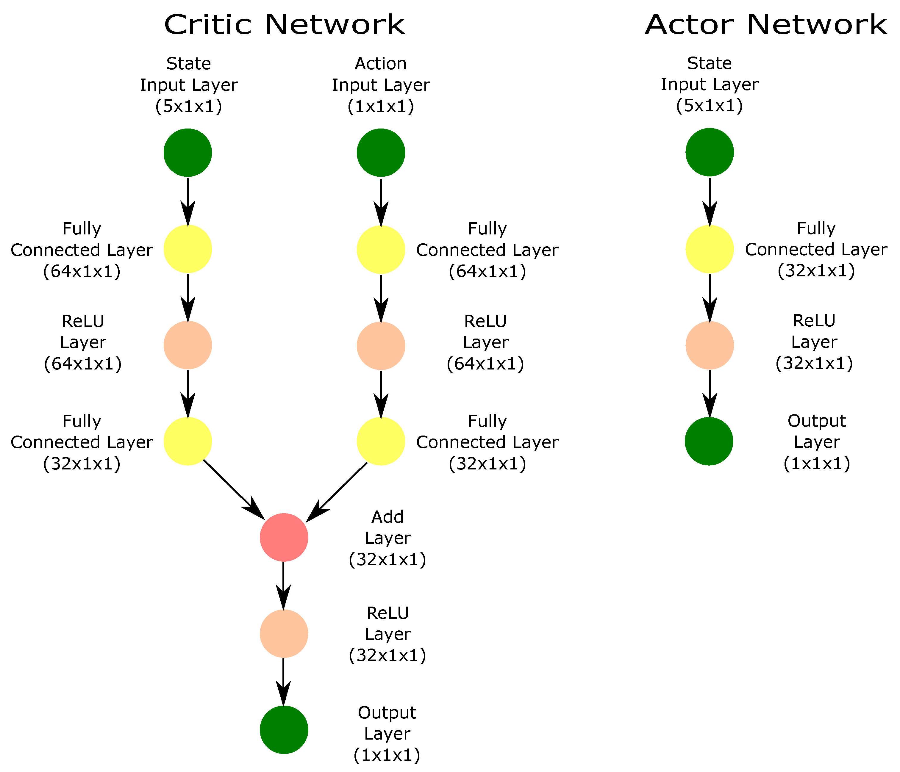
In this section, a control strategy for thermal processes with time delays is presented, integrating NMPC with AC reinforcement learning strategies. Within this framework, NMPC works as a policy generator, providing the trajectory tracking and disturbance rejection objectives to guide the AC agent throughout the learning process. The reward function is derived from the cost function typically formulated in the NMPC optimization problem, ensuring that the AC agent learns to evaluate control actions based on the same performance criteria that govern the baseline controller. The AC agent, implemented through either the deep deterministic policy gradient (DDPG) or twin delayed deep deterministic policy gradient (TD3) methods, assesses control performance by measuring how effectively the thermal process tracks the reference trajectory while simultaneously adapting to disturbances and system uncertainties in real time.

The integration is not only aimed at improving the agent’s learning efficiency but also at enabling adaptive control adjustments based on feedback from the process. Moreover, the proposed controller eliminates the need to compute a terminal cost during the control execution, which is typically required in NMPC and can be computationally intensive for nonlinear system dynamics. By leveraging AC-based approaches, the proposed method enhances adaptability to model uncertainties and varying process conditions, ensuring that the control strategy remains effective even in unpredictable operating environments. In addition, the combination of NMPC and AC strategies is designed to reinforce robust control performance while preserving system stability.

4.1. Observation and Action Spaces

Reinforcement learning (RL) techniques rely on MDPs to model system dynamics, where decisions are made based on the assumption of full state observability. Similarly, NMPC requires an observable model to predict future system behavior and optimize control actions accordingly. Therefore, establishing a state space representation with appropriate state and control actions is essential to ensure that the DRL agent can learn an effective policy aligned to NMPC objectives. In a standard MDP framework, the AC agent has direct access to the complete state of the environment. However, in the case of the thermal process of this work, full observability is not feasible due to inherent system constraints. Instead, the agent must infer the system state from a set of measurable process variables. Then, the observations for the proposed controller are given by

$$o=\{e_T,e_T^i,e_T^d,T,T_d\}$$

(21)

where $e_T$ represents the temperature error of the thermal process computed by $e_T=T_d-T$, with reference temperature $T_d$ and measurable sensor temperature T; $e_T^i$ stands for the continuous integral error given by $e_T^i=\int e_{T}dt$; $e_T^d$ is the continuous derivative error obtained with $e_T^d={\displaystyle \frac{d{e}_T}{dt}}$. All these observations are standardized within the [−1, 1] range to ensure equal prioritization of learning across the scaling factors. Based on the process constraints, the system state space and control action space operate according to intrinsic temperature limits and specified input ranges, respectively. Specifically, the action space is defined here by $a=\left\{Q_u\right\}$, where $Q_u$ works as a control input associated with the heat input as a percentage. Such operating margins for the states and control action are summarized in

Table 2. State and control input constraints of the thermal process.

Parameter	Description	Min	Max
$e_T$	Temperature error	−50 C°	50 C°
T	Measured temperature	273 + 24.5 K°	273 + 50 K°
$T_d$	Reference temperature	273 + 24.5 K°	273 + 50 K°
$Q_u$	Percentage heater input	0%	100%

.

4.2. Nonlinear Model Predictive Control-Driven Reward Strategy

To optimize long-term reward returns in alignment with control objectives, the proposed reward function is formulated based on a NMPC cost function, prioritizing the minimization of both tracking errors and control effort. The agent is designed to improve trajectory tracking accuracy while efficiently regulating control inputs, ensuring robust performance against external disturbances and model uncertainties. Moreover, the agent dynamically adapts the learning to varying process conditions, mitigating the influence of disturbances during control execution. Consequently, the reward function is defined as the minimization of a stage cost function associated with a nominal NMPC problem, explicitly formulated to achieve the desired control objectives. Since the agent is trained using this reward function, the NMPC objectives are implicitly addressed through the minimization of trajectory tracking errors and control effort, subject to feasible state and input constraints. By integrating the reward function within the DRL framework, the proposed approach preserves the advantageous properties of NMPC while leveraging DRL techniques to enhance robustness against disturbances and uncertainties.

The cost function J that captures the integral control objectives of trajectory tracking and control effort is detailed in Equation (22), where $(\overline{x}$ and $\overline{u}$ comprise the nominal system states and control input (i.e., disturbance-free), respectively. $T_p$ is the prediction horizon, and $T_c$ is the control horizon. To compute the control input $\overline{u}$, an optimization problem (OP) associated with the nominal system dynamics in Equation (1) is proposed by

$$\begin{array}{c}\hfill \underset{\overline{u}(·)}{min}J(\overline{x}\left(t\right),\overline{u}(·);T_c,T_p)\end{array}$$

(22)

with:

$$\begin{array}{c}\hfill J(\overline{x}\left(t\right),\overline{u}(·);T_c,T_p):={\int }_t^{t+T_p}l(\overline{x}\left(\tau \right),\overline{u}\left(\tau \right))d\tau +V_N\left(\overline{x}(t+T_p)\right)\end{array}$$

(23)

subject to:

$$\begin{array}{cc}\hfill \dot{\overline{x}}\left(\tau \right)& =f(\overline{x}\left(\tau \right),\overline{u}\left(\tau \right)),\overline{x}\left(t\right)=x\left(t\right)\hfill \\ \hfill \overline{u}\left(\tau \right)& =\overline{u}(\tau +T_c),\forall \tau \in [t+T_c,t+T_p]\hfill \\ \hfill \overline{x}\left(t\right)& \in \mathcal{X},\forall \tau \in [t,t+T_p]\hfill \\ \hfill \overline{u}\left(\tau \right)& \in \mathcal{U},\forall \tau \in [t,t+T_c]\hfill \end{array}$$

where $T_p$ and $T_c$ represent the state prediction and control horizon, respectively. The term l denotes the stage cost function that captures the control objectives, whereas $V_N$ denotes the terminal cost function, which was incorporated during the training phase to ensure stability of the closed-loop system by penalizing deviations from the desired terminal state. While the terminal cost $V_N$ played a critical role in shaping the NMPC-generated trajectories used for training, its explicit design and evaluation were not required during policy execution. Specifically, once the DRL policy was learned, the terminal cost was no longer explicitly evaluated at runtime. Instead, the agent learned from the terminal state trajectories within the control policy through reward shaping and repeated exposure to NMPC-guided episodes, enabling the execution of a stable control policy without requiring online computation of $V_N$. To ensure feasibility throughout the optimization process and meet the control requirements of the thermal system described in Equation (1), the agent first verifies that the state constraints $\mathcal{X}$ and control input constraints $\mathcal{U}$ are satisfied. Such constraints are given by

$$\begin{array}{cc}\hfill & \mathcal{X}:=\{\overline{x}\in {\mathbb{R}}^n|x^{\min }\le \overline{x}\le x^{\max }\}\hfill \end{array}$$

(24)

$$\begin{array}{cc}\hfill & \mathcal{U}:=\{\overline{u}\in {\mathbb{R}}^m|u^{\min }\le \overline{u}\le u^{\max }\}\hfill \end{array}$$

(25)

The stage cost function l encompasses the control objectives of the NMPC controller, which are integrated into the DRL framework for learning tracking and regulation capabilities through exploration and exploitation of the environment, including the minimization of tracking errors and the smoothing of the control input effort. Such a cost function can be described as follows:

$$\begin{array}{cc}\hfill l(\overline{x},\overline{u})& ={({\overline{x}}^{\mathrm{ref}}-\overline{x})}^{T}S({\overline{x}}^{\mathrm{ref}}-\overline{x})+{({\overline{u}}^{\mathrm{ref}}-\overline{u})}^{T}R({\overline{u}}^{\mathrm{ref}}-\overline{u})\hfill \end{array}$$

(26)

$$\begin{array}{cc}\hfill V_N\left(\overline{x}(t+T_p)\right)& ={({\overline{x}}^{\mathrm{ref}}-\overline{x})}^T{P}_N({\overline{x}}^{\mathrm{ref}}-\overline{x})\hfill \end{array}$$

(27)

where ${\overline{x}}^{\mathrm{ref}}$ and ${\overline{u}}^{\mathrm{ref}}$ denote state and control input set points, respectively, which are fixed for each episode but changed throughout the training process. In general, weights S and R denote positive definite symmetric matrices which provide the ability to tune nominal control performance through the balance between the tracking error and control input effort. It is worth noting that the matrix $P_N$ is often challenging to compute for nonlinear systems without introducing increased conservativeness, and thus, it is treated as a design parameter. Additionally, due to the inherent non-convexity of the optimization problem caused by nonlinear model constraints, global optimality cannot be guaranteed.

From the DRL perspective, the agent is designed to learn from the nonlinear model following the control objectives raised in an NMPC scheme. Indeed, the control objective for the agent is to use an internal optimization process while adjusting the reward policy according to the stage cost function of the NMPC. The NMPC works as a policy generator, while the DRL strategies evaluate the learning process. Thus, the optimization process incorporates the state $\mathcal{S}$ and action $\mathcal{A}$ constraints into the learning process, as defined in Equation (24) and Equation (25), respectively, and they are specified as follows:

$$\begin{array}{cc}\hfill \mathcal{S}& :=\{s\in {\mathbb{R}}^m|T^{\min }\le s\le T^{\max }\}\hfill \end{array}$$

(28)

$$\begin{array}{cc}\hfill \mathcal{A}& :=\{a\in {\mathbb{R}}^n|Q_u^{\min }\le a\le Q_u^{\max }\}\hfill \end{array}$$

(29)

Given that the agent’s goal is to iteratively optimize the NMPC objectives in terms of tracking and disturbance rejection, the optimization problem described in Equation (22) can be reformulated to integrate the NMPC cost function within a reward policy iteration framework. However, rather than directly optimizing the cost function J as part of the DRL process, the reward function is designed to ensure that the agent achieves at least the same control objectives that the NMPC strategy targets. This ensures that the learning process remains aligned with the NMPC framework while avoiding the need for building a simultaneous control framework that accounts for additional compensatory or corrective control actions. Specifically, the agent aims to minimize the cost function J, but rather than directly computing optimal control inputs at each iteration, it relies on a reward function derived from the optimized NMPC cost as follows:

$$r_{NMPC}(s_t,a_t):=-{\int }_t^{t+T_p}l(T\left(\tau \right),Q_u\left(\tau \right))d\tau -V_N\left(T(t+T_p)\right)$$

(30)

where $l(T\left(\tau \right),Q_u\left(\tau \right))$ represents the stage cost, penalizing both tracking errors and control effort, while $V_N\left(T(t+T_p)\right)$ accounts for the terminal cost function addressed to ensure the system stability along the training process. These cost functions are given by

$$\begin{array}{cc}\hfill l(T,Q_u)& ={(T^{\mathrm{ref}}-T)}^{T}S(T^{\mathrm{ref}}-T)+Q_u^{T}R{Q}_u\hfill \end{array}$$

(31)

$$\begin{array}{cc}\hfill V_N\left(T(t+T_p)\right)& ={(T^{\mathrm{ref}}-T)}^T{P}_N(T^{\mathrm{ref}}-T)\hfill \end{array}$$

(32)

It is worth mentioning that, although the DRL agent does not explicitly solve an optimization problem at each time step, the NMPC remains active throughout the learning process. Consequently, the training stage inherently involves optimization steps for each learning episode; however, the training process remained feasible within practical time constraints. To accelerate the learning process and improve convergence, reward shaping is incorporated by adding an additional shaped reward $\tilde{r}$, which provides intermediate feedback on the trajectory tracking improvement and control smoothness. Then, the final reward function is expressed as

$$r=r_{NMPC}+\lambda ·\tilde{r}$$

(33)

where $\lambda \in [0,1]$ is a weighting factor that balances the influence of the NMPC cost function and the shaped reward $\tilde{r}$. This shaped reward enables residual learning, allowing the agent to learn from both the global NMPC cost function J and the local trajectory improvements provided by $\tilde{r}$, thereby effectively reducing the dependence on frequent NMPC evaluations. The parameter $\lambda$ was selected through a heuristic approach to balance the influence of the NMPC-based reward and the shaped reward r. To this end, a set of candidate values within the range [0, 1], incremented by 0.1, was evaluated during preliminary simulations. These simulations assessed control performance and stability in terms of cumulative reward and sensitivity to the shaped reward. Based on this assessment, $\lambda =0.3$ was identified as the suitable value to be fixed, as it consistently yielded smooth learning and improved trajectory tracking with reduced oscillatory responses during early training. The shaped reward can be defined as a function of the instantaneous tracking error ${\epsilon }_z\left(t\right)$ and control input effort ${\epsilon }_u\left(t\right)$:

$$\tilde{r}=-\alpha ·{\epsilon }_z\left(t\right)-\beta ·{\epsilon }_u\left(t\right)$$

(34)

where $\alpha$ and $\beta$ are positive constants that regulate the penalization of the actual tracking errors and control effort, respectively. The tracking error ${\epsilon }_z\left(t\right)$ and the deviation of the control input from the previous input ${\epsilon }_u\left(t\right)$ are given by:

$$\begin{array}{cc}\hfill {\epsilon }_z\left(t\right)& = \parallel z^{\mathrm{ref}}\left(t\right)-\overline{z}\left(t\right)\parallel \hfill \end{array}$$

(35)

$$\begin{array}{cc}\hfill {\epsilon }_u\left(t\right)& = \parallel u^{\mathrm{ref}}\left(t\right)-\overline{u}(t-1)\parallel \hfill \end{array}$$

(36)

To improve convergence and learning with the proposed shaped rewards, NMPC generates optimal control sequences for a set of representative initial conditions. These precomputed solutions initialize the policy and value function approximations for the DRL agent, particularly during the early exploration phase. This approach reduces computational overhead while ensuring near-optimal performance and control feasibility. As the DRL agent learns the control policy, the need for real-time NMPC optimization is reduced, allowing the system to operate with minimal computational cost.

The constraint values and NMPC parameters used in the NMPC-based reward policy function, following tuning for the thermal process, are presented in

Table 3. Parameters for the NMPC-based reward model.

Parameter	Description	Value
$T^{\min }$	Lower bound state limit	273 + 24.5 K°
$T^{\max }$	Upper bound state limit	273 + 50 K°
$Q^{\min }$	Lower bound control input limit	0%
$Q^{\max }$	Upper bound control input limit	100%
$T_p$	Prediction horizon	20
$T_c$	Control horizon	5
S	State weight parameter	0.01$I_3$
R	Control input weight parameter	0.001
$P_N$	Stabilizing state parameter	0.15$I_3$

. The computational burden of the proposed control agent typically escalates by increasing the prediction horizon $T_p$ and control horizon $T_c$. However, selecting a relatively small $T_p$ can degrade control performance, as the agent may fail to adequately learn tracking and regulation. Conversely, an excessively large $T_c$ limits the ability to execute timely control actions, which is particularly unfavorable given the inherently long time delay in the thermal system dynamics. To address these trade-offs, the horizon lengths were chosen to balance three critical aspects: (i) efficient agent training, (ii) feasibility for real-time implementation, and (iii) robust control performance, particularly under long and variable time delays characteristic of the thermal process. Since the thermal system exhibits relatively slow reaction dynamics in response to reference changes, a confident horizon length was enough to ensure stability. For consistency across all NMPC-based strategies, the prediction and control horizons were set to $T_p=20$ and $T_c=5$, respectively.

Remark 1.

It is worth highlighting that the terminal cost function, embedded within the NMPC-based reward formulation, was used exclusively during the training phase. Its role was to guide the agent toward stable trajectory generation, leveraging the long-term control objectives associated with NMPC. While a terminal cost term is conventionally included to guarantee theoretical stability under specific model formulations [45], the proposed approach avoids the need for explicit terminal evaluation at runtime. Instead, closed-loop stability emerges from the agent’s learned policy, shaped through repeated exposure to NMPC-generated trajectories and rewards that penalize deviations from the reference. During training, the agent effectively internalized terminal state behavior by being penalized for persistent tracking errors in response to reference variations and external disturbances, thereby ensuring stable performance during deployment without online computation of the terminal cost function $V_N$. In addition, this approach enabled the proposed controllers to adapt the thermal dynamics to time-varying conditions without need of additional compensatory control actions to mitigate errors induced by disturbances or model uncertainties. Such perturbations were also inherently addressed by the agent as part of the training process, thereby enhancing the robustness of the control strategy.

4.3. Randomized Episodic Training Approach

To train the AC-based learning models, the thermal dynamics described in Equation (2) were incorporated into the environment, with the system states being represented by the observations o from Equation (21), and the control action a followed the formulation in Section 4.1. The objective of the AC-based framework is to develop an adaptive control agent, independent of its specific learning architecture and capable of accurately tracking reference temperature trajectories while mitigating uncertainties and disturbances inherent to the thermal process. To achieve such a goal, external variability was intentionally introduced into the exploration and exploitation phases by means of a reference shift parameter that changed episodically, randomly changing based on a uniform probability distribution. This strategy was incorporated to enhance exploration under variable reference conditions, as they changed while tracking over time, thus preventing systematic error accumulations in the reward function and mitigating potential estimation biases. Specifically, considering minimum and maximum temperature values and actions that must satisfy the state and control input constraints outlined in Table 2, two previously normalized variables were integrated into the training process: (i) an episodic reference temperature variable $T_{\mathrm{ref}}$, which varied across training episodes for all admissible control inputs, and (ii) an episodic disturbance variable $T_0$, which spanned the largest feasible disturbance range. The training parameterization is defined in terms of a randomly generated parameter $D_{\mathrm{rand}}\in [-1,1]$, such that the episodic variables are structured as follows:

$$\begin{array}{c}\hfill T_{\mathrm{ref}}^{\mathrm{train}}={\displaystyle \frac{1}{2}}(T_d^{\max }-T_d^{\min })(D_{\mathrm{rand}}+3)\end{array}$$

(37)

$$\begin{array}{c}\hfill T_0^{\mathrm{train}}={\displaystyle \frac{1}{2}}(T_d^{\max }-T_d^{\min })(D_{\mathrm{rand}}+3)\end{array}$$

(38)

where $T_{\mathrm{ref}}^{\mathrm{train}}$ denotes the target training temperature, used to train the agent in tracking time-varying reference trajectories. Likewise, $T_0^{\mathrm{train}}$ represents the initial temperature for each training episode, allowing the agent to adapt effectively to varying system conditions. To further enhance robust control performance and strengthen the control system’s ability to reject disturbances, a new episodic parameter is also incorporated into the learning process, as described below:

$$P^{\mathrm{train}}=p\times D_{\mathrm{rand}}$$

(39)

where $P^{\mathrm{train}}\in [-p,p]$ is a stochastic parameter that represents a variable disturbance during training. Similarly, the parameter p stands for the largest feasible bound of disturbances. Note that alternative observations and reward formulations may be used; however, the proposed reward function is suited for achieving satisfactory performance in practice for the delayed thermal process.

5. Experimental Setup and Results

This section outlines the experimental setup used for the training, testing, and validation of the control agents. It also presents the results obtained from the experimental trials, offering a quantitative evaluation and comparative analysis of the control performance of the proposed temperature tracking controllers.

5.1. Environment Setup Description

The experimental setup for the thermal system was based on a dual-heater process with a long, variable time delay, as detailed in [46] (see Figure 1). The thermal process was conducted in a temperature control laboratory (TCLab^® module), which inherently exhibits second-order dynamics. Unlike the nonlinear model that represents the MDP for the design and training of the the proposed DRL-based controllers, a linear model representation of this thermal system was used to obtain forward equations of the dynamical model, which were subsequently used in the testing phase. The experimentation board was interfaced with a microcontroller to collect temperature data and generate pulse width modulation (PWM) signals used as control actions. Specifically, the TCLab^® electronic board was outfitted with two TIP31C NPN bipolar junction transistors (BJTs), mounted in TO-220 packages. Each BJT was paired with a TMP36GZ temperature sensor, providing a voltage output (in mV) linearly proportional to the measured temperature. The heaters were powered by a 5V@2A power supply, delivering a maximum output power of 20 W. Further details regarding the hardware design and implementation are provided in [46,47]. To test the agent design and compare performance, six different controllers were evaluated against step-wise temperature reference changes and external disturbances. The tested controllers included (i) a standard PID controller, widely used in industrial thermal applications [48], with parameters tuned theoretically as outlined in Table 1; (ii) an NMPC strategy [49] with parameters specified in Table 3; (iii) a TD3-based control approach; (iv) a DDPG-based control method; (v) the NMPC-based DDPG strategy; and (vi) the NMPC-based TD3 approach. All comparison controllers and reinforcement learning agents were developed and tested using MATLAB^TM R2024a from MathWorks Inc^© and Simulink (MathWorks Inc., Natick, MA, USA), with the agents trained and simulated in the thermal environment by leveraging the Reinforcement Learning Toolbox [24,50]. The Simulink block diagram for all DRL agents was constructed based on the architecture shown in Figure 4, which defines the control structure for both NMPC–DDPG and NMPC–TD3 controllers.

Four experimental trials were conducted through simulations to assess the control performance and adaptability of the agents. Specifically, one trial focused on a combined strategy of reference tracking and regulation, while the remaining three trials evaluated the robust performance of the agents in temperature regulation tasks, considering (i) external disturbances, (ii) dead time variations, and (iii) changes in the time constant parameters of the thermal process. The first trial involved tracking the reference temperature with one heater while the other was excluded, with the environment initially set to a temperature of $T_0={35}^{\circ }$C and a $30\%$ pulse width modulation (PWM) control input ($Q_u$). The reference temperature was increased and then decreased in consistent steps of $4^{\circ }$C every 100 s, ultimately reaching ${40}^{\circ }$C. The first regulation trial focused on maintaining a reference temperature of $T_0={35}^{\circ }$C using one heater while the system was exposed to non-measurable external temperature disturbances. In the second regulation trial, dead time variations were introduced, ranging from 0 to 100% at 100 s intervals. The third trial specifically tested the proposed control methodology under conditions where the time constant ${\tau }_s$ was varied within a feasible range of parameters. All trials were conducted while simultaneously tracking the previously prescribed reference temperature trajectory.

5.2. Setup of Actor–Critic Agents

The task of analytically setting an optimal AC network architecture that precisely meets learning requirements, such as the number of hidden layers, neurons per layer, and connections, is inherently complex. Therefore, following network configurations previously presented in [51] has guided the design of the proposed scheme. The proposed architecture uses three hidden layers for the critic network and one hidden layer for the actor network, as depicted in Figure 5. Specifically, the critic network consists of an input layer connected to five state variables of the control system, corresponding to the number of observed states defined in Section 4.1. This input is followed by a fully connected layer with 64 neurons and a rectified linear unit (ReLU) activation function. Subsequently, the network bifurcates into two separate paths. One path proceeds through a fully connected layer with 32 neurons, while the other path processes a one-dimensional action input via another 32-neuron fully connected layer. These two paths then converge into an addition layer, which combines the outputs before passing them through an additional fully connected layer with 32 neurons and ReLU activation. The output of the critic network is a single scalar value, which is used to estimate the Q-value for policy optimization. On the other hand, the actor network is designed with a simpler structure with respect to the critic. It accepts the same five-state input layer as the critic network and processes it through a fully connected layer of 32 neurons with ReLU activation. The output layer of the actor network generates continuous action values via a single-output layer. The increased depth and width of both networks are crucial to enhance the feature extraction and representation capabilities of the control system. This is particularly advantageous for handling the continuous action spaces, which are the main characteristics of the AC-based control strategies applied to the thermal process.

The proposed methodologies involved the use of separate actor, critic, and target networks, all employing identical network architectures and the same number of hidden layers. The training process was based on the mean squared error (MSE) loss function, with optimization achieved through stochastic gradient descent. To ensure statistical significance during the training phase, a total of 1500 episodes per scenario were conducted. However, the training for the NMPC-based DDPG and NMPC-based TD3 models reached convergence in approximately 650 and 400 episodes, respectively. The training task was considered complete when the average cumulative reward did not exceed the performance threshold of $r_{\mathrm{mean}}=-1$, at which point the algorithm was stopped. Early stopping was also incorporated into the training process, where the observed variables were continuously monitored to prevent overfitting, particularly when performance on the validation set started to degrade. An example of the reward evolution before the early stopping criterion was applied can be seen in Figure 6, where the blue solid line represents the average reward obtained with the DDPG agent, while the orange line corresponds to the rewards from training the TD3 agent. A summary of the experimental parameters for the AC-based models used in the trials is provided in

Table 4. Experimentally tuned parameters for AC-based controllers, including DDPG and TD3.

Parameters of AC Methods:	DDPG (Values)	TD3 (Values)
Learning rate (actor)	0.003	0.003
Learning rate (critic 1 and 2)	0.003	0.003
Discount factor	0.99	0.99
Buffer size	10,000	10,000
Batch size	128	128
Soft update $\gamma$ (actor and critics)	0.005	0.005
Gradient threshold	1	1
Noise variance	0.03	0.03
Target network update steps	5	5
Total number of episodes (for monitoring purposes)	1500	1500

, with the selection criteria for these parameters discussed in Section 5.3. These parameters were fine-tuned on a high-performance computing platform whose specifications are outlined in

Table 5. Computational setup specifications for the experimentation trials.

Configuration	Values
Operating system	Windows 11 Pro
CPU	i7-8550U
GPU	GeForce 940MX
RAM	16G
Software simulation platform	MATLAB R2023a
Simulation environment	Simulink

. The simulation time for most of the trials exceeded 300 s with the sampling time set to 1 s.

5.3. Criteria for Hyperparameter Selection in Thermal Process Control

The hyperparameters for the training process were selected using heuristics [52,53], addressed to ensure stable learning by maximizing long-term rewards and minimizing tracking errors. Initially, during early tests, the training process hardly demonstrated smooth or stable reward behavior. Then, the first set of experiments was conducted over 5000 episodes. In these initial tests, the agents appeared to converge to a learning solution after a few episodes, as detailed in Section 5.2. However, approximately 1000 episodes after reaching convergence, a destabilization phenomenon occurred, resulting in a significant drop in cumulative reward for both agents. This instability was attributed to certain state conditions in the thermal process that have not been sufficiently explored, and it led to penalties in the learning process. As a consequence, additional training episodes were necessary to mitigate these effects and recover the learning conditions. In terms of control performance, this instability initially presented as a triangular ripple in the temperature variable with a peak-to-peak magnitude ranging from 2 to 4 °C. It was hypothesized that the introduction of random variables during training contributed to this phenomenon. However, these random variables were essential for exploring new reference temperatures in each learning episode. To address this concern, several tests were conducted, where various training parameters were adjusted, including the learning rate (ranging from 0.001 to 0.006 for both the critic and actor networks), the discount factor (between 0.98 and 1), and the batch size (i.e., choices of 64, 128, and 256). Moreover, the complexity of the reward function was progressively increased during training to encompass a broader set of observations, enabling a more comprehensive evaluation of the AC-based control approaches. It was critical to maintain a pre-trained model with successful parameters in order to enable continued training with new configurations. Nevertheless, using this approach for parameter selection, the destabilization phenomenon was effectively eliminated between episodes 1600 and 4500. Based on these results, the total number of training episodes was set to 1500 to ensure convergence while minimizing excessive training time.

5.4. Preliminary Control Performance Evaluation

To compare control performance, a test was conducted using six different control strategies applied to the thermal process. The first strategy involved a proportional integral derivative (PID) controller tuned using the Ziegler–Nichols method [54]. The PID controller used the following gains: $K_p=30.12$, $K_i=24.47$, and $K_d=3.29$. The second strategy used an NMPC strategy, as presented in Section 4.2, with the parameters given in Table 3. In addition to these controllers, two AC-based controllers were tested: DDPG and TD3. Both controllers used reward functions identical to the modified PID, as described in Section 5.2. We also evaluated two hybrid controllers: NMPC-based DDPG and NMPC-based TD3. These hybrid controllers incorporated the NMPC criterion into their reward functions, as detailed in Section 4.2, and their respective training parameters are given in Section 5.2. To assess the performance of each controller, several metrics were used, such as the integral square error (ISE), integral time square error (ITSE), integral absolute error (IAE), and integral time absolute error (ITAE) [39]. The test was conducted over 300 s and included approximately 1500 episodes that combined reference tracking and disturbance rejection criteria. Specifically, step changes in reference temperature were applied at time instants $t=0$ and $t=100$ s, with target temperatures set to $T_{\mathrm{ref}}\left(0\right)={35}^{\circ }$C and $T_{\mathrm{ref}}\left(100\right)={30}^{\circ }$C, respectively. At 200 s, an external disturbance of $T_{\mathrm{dist}}=-4^{\circ }$C was also introduced to evaluate the thermal system’s response.

The results of this preliminary test are shown in Figure 7, and the control performance metrics summarized in

Table 6. Performance metrics obtained while tracking reference trajectories using standard PID, NMPC, and the proposed AC-based controllers, including DDPG- and TD3-based approaches.

Metric	PID	NMPC	DDPG	TD3	NMPC-Based DDPG	NMPC-Based TD3
ISE	$4.136\times {10}^2$	$5.426\times {10}^2$	$3.287\times {10}^2$	$3.339\times {10}^2$	$3.904\times {10}^2$	$3.201\times {10}^2$
ITSE	$1.241\times {10}^5$	$3.811\times {10}^5$	$7.06\times {10}^4$	$8.982\times {10}^4$	$1.171\times {10}^5$	$9.602\times {10}^4$
IAE	$1.765\times {10}^2$	$3.081\times {10}^2$	$1.654\times {10}^2$	$1.552\times {10}^2$	$1.686\times {10}^2$	$1.620\times {10}^2$
ITAE	$4.795\times {10}^4$	$1.143\times {10}^5$	$5.863\times {10}^4$	$4.784\times {10}^4$	$4.950\times {10}^4$	$4.861\times {10}^4$
Settling time	90.21 s	30.71 s	64.1 s	58.18 s	46.9 s	67.49 s
Overshoot	39.7%	14.5%	21.9%	32.4%	21.4%	20.15%
Rise time	4.1 s	4.81 s	3.84 s	5.01 s	8.1 s	3.45 s
Dead time	0.31 s	0.03 s	0.28 s	0.01 s	0.25 s	0.24 s

. The PID controller demonstrated a variable and oscillatory response to reference changes and external disturbances. However, the thermal process was able to recover from disturbances, stabilizing the thermal dynamics. In contrast, the NMPC strategy successfully tracked the reference trajectory, maintaining stable performance during both increases and decreases in the reference temperature. While NMPC was effective in tracking the temperature reference, it showed high sensitivity to external disturbances. This sensitivity led to abrupt transient responses and maintained steady-state deviations from the reference trajectory. In comparison, the DDPG controller showed an improvement in control performance in terms of tracking and disturbance rejection.

As shown in Table 6, the DDPG approach achieved a significant reduction in tracking error, with an ISE of 568.7. This value represents a 22.5% reduction compared to NMPC (ISE = 1401) and a 22.6% improvement over PID (ISE = 734.4), highlighting the DDPG’s ability to track the reference temperature with a lower temperature error. The DDPG controller also outperformed the other strategies in the ITSE metric, achieving a value of 17.06 $\times {10}^5$ This represents a 22.5% improvement over NMPC (42.04 $\times {10}^5$) and is 22.5% better than PID (22.03 $\times {10}^5$). The TD3 controller exhibited even better performance, with an ISE of 477.1, which is 35.5% better than DDPG and more effective than both NMPC and PID. Additionally, both the NMPC-based DDPG (ISE = 705.4) and NMPC-based TD3 (ISE = 616.0) controllers showed substantial improvements, indicating the benefit of combining NMPC with reinforcement learning strategies. Regarding settling time, NMPC demonstrated a significant reduction, with a settling time of 30.67 s—65.4% faster than PID’s 88.55 s. Although NMPC-based TD3 showed an improved settling time of 68.4 s, it was still slower than the DDPG-based methods.

Figure 8 presents a comparison of control performance in the preliminary test. This evaluation was performed based on the results of control metrics Integral of Absolute Error (IAE), Integral of Time-weighted Absolute Error (ITAE), Integral of Squared Error (ISE), and Integral of Time-weighted Squared Error (ITSE). The proposed controllers effectively demonstrated their ability to track the desired temperature profile and mitigate the impact of external disturbances. Most of the AC-based controllers performed well in tracking the reference temperature, with the exception of the DDPG controller, which exhibited larger steady-state errors at certain operational reference points (as shown in the DDPG response during the first 100 s in Figure 7). This behavior in the DDPG controller can be attributed to control actions derived from the policy that were not fully adapted to the temperature tracking errors encountered during training. However, this limitation was completely addressed by integrating NMPC, which offers feedback by penalizing predicted errors based on future system dynamics (as shown in the comparison with the NMPC-based controllers within the same time frame). The AC-based controllers successfully compensated for errors while tracking the reference temperature and counteracting external disturbances, effectively demonstrating their ability to return to the reference temperature even in the presence of thermal disturbances.

5.5. Test of Reference Temperature Changes

From the preliminary assessment discussed in Section 5.4, only the AC-based methods were selected for a more in-depth analysis, focusing in this case on tracking performance in reference temperature control. The experimental setup involved tracking a reference with a step-wise time-varying temperature profile, composed of both incremental and decremental step changes. Essentially, step transitions of the reference temperature $T_{\mathrm{ref}}$ were tested at $t=\{0,100,200,300,400\}$ seconds, with respective setpoints of 30, 32, 36, 40, and 35 °C. This configuration was designed to evaluate the adaptability and consistency of the learned control policies under dynamic reference conditions. As illustrated in Figure 9 and summarized in

Table 7. Performance metrics of the proposed temperature controllers obtained from trajectory tracking tests.

Metric	DDPG	TD3	NMPC-Based DDPG	NMPC-Based TD3
ISE	7.812 $\times {10}^1$	8.421$\times {10}^1$	10.2$\times {10}^1$	7.541$\times {10}^1$
ITSE	3.001$\times {10}^4$	3.991$\times {10}^4$	4.985$\times {10}^4$	3.851$\times {10}^4$
IAE	22.71$\times {10}^1$	20.12$\times {10}^1$	19.51$\times {10}^1$	17.84$\times {10}^1$
ITAE	10.81$\times {10}^4$	10.24$\times {10}^4$	11.2$\times {10}^4$	8.95$\times {10}^4$

, the results verified that most of the evaluated agents were able to track the imposed reference trajectory. For instance, for each reference temperature change, the NMPC-based TD3 agent consistently achieved the best control performance in terms of tracking accuracy, outperforming the other baseline methods such as the standard DDPG, TD3, and NMPC-based DDPG. A notable case occurred in the DDPG control performance during the final segment of the test (i.e., 400–500 s), where persistent tracking errors emerged at specific operating temperature points.

Although the discrepancy was eventually corrected by the DDPG controller, it revealed a delayed adaptation, which can often be attributed to the agent’s limited exposure to a diverse set of initial temperature reference conditions during the training phase. Consequently, this constrained exploration led to a suboptimal policy that mainly relied on previously learned control mappings without adjusting effectively to unforeseen reference transitions. A summarized radar-based analysis was developed in Figure 10 founded on control metrics. The graphical and numerical results illustrate that the NMPC-based TD3 controller exhibited improved generalization across reference changes compared to both DDPG and the standard TD3. This controller consistently tracked positive and negative step transitions of temperature and generally achieved regular peak responses. Notably, during the interval from 300 to 400 s, TD3-based methods showed a faster transient response and more accurate tracking performance when compared to DDPG-based methods. Indeed, DDPG exhibited delayed convergence, and NMPC-based DDPG showed persistent deviations from the reference temperature. Moreover, the reduced steady-state error observed in both the TD3 and NMPC-based TD3 implementations underscores the effectiveness of these controllers in refining control effort over time, leading to asymptotically stable behavior under reference disturbances. The NMPC-based TD3 performance highlighted the advantage of incorporating NMPC into DRL frameworks for trajectory tracking in thermal systems, as it provides a principled optimization structure that enhanced policy learning across varying temperature references. The use of twin critics and delayed policy updates in TD3 further contributed to stable learning dynamics. Such integration also resulted in smoother actions and a reduction of oscillatory responses with respect to DDPG, exhibiting improved closed-loop performance. The integration of model-based cost shaping in the reward structure further contributed to this improvement while tracking step-wise reference temperature, enabling the NMPC-augmented agents to exploit both global optimization criteria and local policy corrections through residual learning. Nevertheless, NMPC-based DDPG required a more exploratory stage to further improve learning capabilities when compared to NMPC-based TD3. These results verified the feasibility of using NMPC-informed reinforcement learning policies to reduce tracking error, accelerate convergence, and ensure reliable control performance in nonlinear thermal processes.

5.6. Test of Robustness Against External Disturbances

This test was designed to evaluate the robust control performance of the thermal system in the presence of external disturbances, focusing on the system’s ability to maintain stability and regulation despite perturbations. Disturbances were intentionally introduced into the system’s dynamics, constrained to remain within the maximum operating range, as indicated by the dashed black lines in Figure 11. A reference temperature of 35 °C was maintained throughout the thermal process, with cumulative disturbances applied at 100, 200, and 300 s with values of 3, 1, and −5 °C, respectively. For all AC-based controllers (i.e., DDPG, TD3, NMPC-based DDPG, and NMPC-based TD3), the thermal control system demonstrated effective disturbance rejection, successfully recovering the system response to the reference temperature and exhibiting consistent peak responses, regardless of whether the disturbances caused an increase or decrease in temperature. From examination, it can be seen that the combination of NMPC and TD3 exhibited better control performance compared to the other AC-based control strategies when regulating the thermal process with long, variable time delays. The integration of NMPC with TD3 resulted in enhanced disturbance rejection due to faster and more accurate tracking responses, characterized by reduced settling time and minimal overshoot. Indeed, the system’s response with NMPC-based TD3 was more stable regardless of whether the temperature deviation was positive or negative, even as different dynamic responses were observed for the other test controllers under the same disturbance occurrence. The use of NMPC with TD3 for controlling the thermal process proved particularly advantageous in handling long time delays, which often lead to inaccuracies and potential instability in traditional control methods. This hybrid approach not only maintained the reference temperature but also improved the system’s ability to adapt to environmental disturbances efficiently, demonstrating the potential of combining NMPC with DRL techniques for real-time control and adaptive regulation against thermal disturbances.

The quantitative analysis of control performance presented in

Table 8. Performance comparison of the the proposed controllers using the AC models under external disturbance conditions.

Metric	DDPG	TD3	NMPC-Based DDPG	NMPC-Based TD3
ISE	14.77$\times {10}^1$	7.806$\times {10}^1$	12.19$\times {10}^1$	7.107$\times {10}^1$
ITSE	7.385$\times {10}^4$	3.903$\times {10}^4$	6.097$\times {10}^4$	3.553$\times {10}^4$
IAE	10.32$\times {10}^1$	4.587$\times {10}^1$	6.988$\times {10}^1$	5.888$\times {10}^1$
ITAE	5.152$\times {10}^4$	2.794$\times {10}^4$	3.349$\times {10}^4$	2.944$\times {10}^4$

demonstrated that the NMPC-based TD3 controller outperformed its counterparts across several metrics, achieving an IAE of 58.8, which is significantly lower than that obtained with DDPG (i.e., IAE = 103.2) and the one attained with NMPC-based DDPG (i.e., IAE = 69.8). Such a IAE improvement indicated the effectiveness of reducing steady-state errors in the regulation of the thermal system dynamics. The TD3 approach and NMPC-based TD3 yielded lower ISE values compared to DDPG and NMPC-based DDPG. This indicates that TD3 controllers generally produce a smaller cumulative error, suggesting that TD3 approaches are more resilient to error accumulation due to external disturbances. In addition, the NMPC-based TD3 approach presented an ITAE of 2.94 $\times {10}^4$, which is lower than that obtained with DDPG (i.e., 5.152 $\times {10}^4$) and NMPC-based DDPG (i.e., 3.34 $\times {10}^4$), strengthening the robust control performance. Although the TD3 approach exhibited comparable performance to NMPC-based TD3 in terms of ISE and ITSE, the NMPC-based TD3 excelled across a broader range of the test metrics, encompassing IAE and ITAE. This highlights the achieved control robustness and the effectiveness of the NMPC-based TD3 approach in comparison to the standard TD3. Analogous robust performance outcomes were achieved with TD3 and DDPG, since their learning model architectures follow related characteristics, but all metrics from the models based on TD3 consistently outperformed all those based on DDPG. In general, when comparing agents with the same AC architecture but different control policy approaches, NMPC-based agents demonstrated enhanced performance metrics, indicating that the NMPC strategy also contributed to the robustness of the control system against disturbances and long time delays. Figure 12 presents the integration results of NMPC with TD3, showing lower values in ISE, ITSE, and ITAE compared to the standalone DDPG and TD3 controllers. This performance outcome highlights the effectiveness of combining NMPC with DRL strategies. In particular, the integration leverages NMPC’s capability to track the reference trajectory against thermal disturbance, while TD3 contributes improved stability and sample efficiency through its twin critic structure. This hybrid approach resulted in robust control performance, the best disturbance rejection, and reduced tracking errors over time, making it suitable for the delayed dynamics of thermal systems.

5.7. Test of Robustness Under Variable Dead Time Effects

This section presents a detailed analysis of robust control performance in the presence of time-delay effects, incorporating classical PID and NMPC strategies to enable a comparative assessment against AC-based controllers. The objective is to evaluate each controller’s capacity to handle inherent system delays and their impact on reference tracking and closed-loop stability, and to achieve this using the step-based temperature reference introduced in Section 5.6. The system’s nonlinear dynamics were modeled using the CFOTD formulation in Equation (4) with an estimated nominal dead time of ${\theta }_s=1.45\mathrm{s}$. To ensure that the evaluation considered a broad scope of control adaptability under non-ideal operating conditions, the validation model of the thermal process was subjected to dead time perturbations of up to 100% relative to the nominal delay. The AC-based control policies were previously trained using variable reference temperatures and external disturbances (as outlined in Section 4.3); however, no internal process variation—such as changes in time delay—was introduced during training. This setup enabled a fair and rigorous evaluation of each controller’s generalization capability under mismatched model conditions. During testing, all AC-based controllers were exposed to identical reference profiles and system parameters, providing a consistent basis for comparison with baseline controllers. The resulting trajectory tracking responses are illustrated in Figure 13, and the associated performance metrics are summarized in

Table 9. Performance metrics obtained when testing the proposed controllers under dead time changes.

Metric	PID	NMPC	DDPG	TD3	NMPC-Based DDPG	NMPC-Based TD3
ISE	19.33$\times {10}^2$	8.355$\times {10}^2$	4.245$\times {10}^2$	2.095$\times {10}^2$	3.87$\times {10}^2$	3.31$\times {10}^2$
ITSE	9.677$\times {10}^5$	4.177$\times {10}^5$	2.122$\times {10}^5$	1.047$\times {10}^5$	2.83$\times {10}^5$	1.66$\times {10}^5$
IAE	8.339$\times {10}^2$	5.578$\times {10}^2$	2.774$\times {10}^2$	1.214$\times {10}^2$	2.358$\times {10}^2$	1.805$\times {10}^2$
ITAE	41.7$\times {10}^4$	27.89$\times {10}^4$	13.87$\times {10}^4$	6.071$\times {10}^4$	12.6$\times {10}^4$	9.026$\times {10}^4$

. The results highlight the enhanced robustness of AC-based strategies when rejecting dead time disturbances, demonstrating improved control performance compared to conventional PID and NMPC techniques under the same evaluation conditions.

As illustrated in Figure 13, the trajectory tracking performance under variable dead time conditions reveals significant differences among the tested control strategies. The PID controller exhibited a consistently oscillatory temperature response, resulting in the highest tracking errors across all scenarios. These oscillations can be attributed to the intrinsic limitations of the PID structure, which fails to account for time delay variations. The presence of dead time introduces a temporal disconnection between the control input and its effect on the system output, causing the controller to continuously overcompensate. This behavior tends to compromise the stability of the controller during the regulation process. Since the PID gains were tuned based on the nominal system delay, any deviation from this configuration impaired the controller’s responsiveness and predictability under changed conditions. In contrast, the NMPC controller avoided oscillatory transients for any operating reference point; however, it was unable to fully eliminate steady-state errors while tracking the reference changes. Actually, the system response exhibited sensitivity of model-based controllers to unmodeled dynamics, as the internal model could not fully capture the time-varying nature of the long time delay. In particular, the internal model did not fully capture the evolving delay characteristics, limiting its ability to generate optimal control actions over the prediction horizon. Consequently, the control inputs computed by the optimization routine were suboptimal, leading to persistent tracking deviations. On the other hand, the AC-based strategies and, in particular, the NMPC-enhanced TD3 controller achieved enhanced performance in terms of ISE and ITAE. These results emphasize the effectiveness of integrating reinforcement learning with model predictive control, as the learned policy demonstrated large adaptability to time delay variations and dynamic system responses, resulting in improved tracking accuracy and robustness.

According to Table 9, the AC-based controllers consistently exhibited low tracking errors despite substantial variations in the system’s dead time. This consistent performance can be attributed to the inherent capacity of actor–critic (AC) agents to learn adaptive control policies from a broad range of dead time changes, allowing them to generalize effectively to previously unseen disturbances and temporal misalignment between control input and system response. Such generalization capability is particularly advantageous in the thermal system of the TCLab module, where the transistor’s nonlinear heat transfer dynamics are highly sensitive to input delays and parameter variations. Notably, although DDPG and TD3-based strategies yielded higher ITAE values (i.e., 13.87 $\times {10}^4$ and 6.07 $\times {10}^4$, respectively) than their NMPC-integrated counterparts, they still outperformed traditional controllers such as PID and NMPC under similar operating conditions. Furthermore, the NMPC-based TD3 approach achieved the lowest ITSE and ITAE values (i.e., 1.66 $\times {10}^5$ and 9.02 $\times {10}^4$, respectively), indicating its enhanced ability to attenuate cumulative errors even in the presence of varying dead time. These results demonstrate the benefit of integrating NMPC with AC-based controllers, particularly while handling a nonlinear thermal system where the interaction between control inputs and heat propagation is delayed and nonlinear. While the NMPC component offers predictive capabilities for handling system constraints and model-based predictions, the DRL agents continuously refined the control policy based on observed performance, resulting in improved stability and tracking accuracy. Additionally, the NMPC-based DDPG controller demonstrated closeness to reference temperatures, with only marginal increases in the instantaneous and accumulated errors. This indicates that combining NMPC with AC-based methods can significantly enhance control robustness, particularly for thermal systems with time-varying dynamics and long time delay effects.

5.8. Test of Robustness Based on Time-Constant Changes

This experiment is designed to assess the robustness of the control strategies under variations in the system’s time constant, which directly affect the dynamic behavior of the thermal process. The evaluation employs the simplified nonlinear thermal model described in Equation (4), where the nominal time constant is defined as ${\tau }_s=9.41$ s. To examine sensitivity to model parameter deviations, two additional extreme values were introduced: ${\tau }_{s,\max }=13.1$ s and ${\tau }_{s,\min }=6.2$ s. These boundary cases provide a rigorous framework to investigate the controllers’ performance under both slower and faster thermal dynamics. The tracking performance was tested using the same reference temperature profile described in Section 5.5. Figure 14 and Figure 15 illustrate the system responses under ${\tau }_{s,\max }$ and ${\tau }_{s,\min }$ conditions, respectively. The results clearly demonstrate that the AC-based controllers outperformed both PID and NMPC strategies in terms of reference tracking and disturbance rejection. Specifically, the PID controller exhibited the largest overshoot and transient deviations when the time constant increased, while the NMPC struggled to reach the reference temperature effectively under the faster dynamics associated with ${\tau }_{s,\min }$. In contrast, the AC-based controllers maintained smoother trajectories and lower steady-state errors regardless of the time constant variation. These findings are quantitatively validated by the performance metrics summarized in

Table 10. Performance metrics obtained from the proposed controllers under time constant changes.

Time Constant	Metric	PID	NMPC	DDPG	TD3	NMPC-Based DDPG	NMPC-Based TD3
6.2 s	ISE	5.204$\times {10}^2$	36.60$\times {10}^2$	4.24$\times {10}^2$	1.25$\times {10}^2$	4.45$\times {10}^2$	1.85$\times {10}^2$
	ITSE	3.02$\times {10}^5$	19.8$\times {10}^5$	2.12$\times {10}^5$	0.65$\times {10}^5$	2.22$\times {10}^5$	0.54$\times {10}^5$
	IAE	3.01$\times {10}^2$	10.27$\times {10}^2$	2.77$\times {10}^2$	0.76$\times {10}^2$	2.06$\times {10}^2$	0.89$\times {10}^2$
	ITAE	15.04$\times {10}^4$	63.74$\times {10}^4$	13.8$\times {10}^4$	3.81$\times {10}^4$	10.33$\times {10}^4$	4.82$\times {10}^4$
13.1 s	ISE	6.89$\times {10}^2$	13.72$\times {10}^2$	5.1$\times {10}^2$	3.26$\times {10}^2$	4.57$\times {10}^2$	4.44$\times {10}^2$
	ITSE	2.44$\times {10}^5$	6.85$\times {10}^5$	2.55$\times {10}^5$	3.63$\times {10}^5$	2.26$\times {10}^5$	1.22$\times {10}^5$
	IAE	2.49$\times {10}^2$	6.98$\times {10}^2$	2.98$\times {10}^2$	3.01$\times {10}^2$	2.8$\times {10}^2$	2.28$\times {10}^2$
	ITAE	1.25$\times {10}^4$	34.92$\times {10}^4$	1.49$\times {10}^4$	2.09$\times {10}^4$	1.4$\times {10}^4$	1.14$\times {10}^4$

, which consolidate the enhanced robustness of AC-based approaches when facing significant variations in system dynamics.

As demonstrated in the previous evaluations, the NMPC controller faced significant challenges when attempting to counteract internal disturbances in the thermal dynamics. Similarly, the PID controller presented intended limitations when exposed to variations in the time constant parameters, as illustrated in Figure 14 and Figure 15. Specifically, in Table 10, the ISE metric indicates that the NMPC controller struggled to maintain performance under both time constant disturbances, unlike the AC-based control approaches, with ISE values of 36.6 $\times {10}^2$ and 13.72 $\times {10}^2$ for ${\tau }_{s,min}$ and ${\tau }_{s,max}$, respectively. In contrast, the PID controller produced even higher ISE values with respect to NMPC, which suggests a reduced ability to minimize errors under similar conditions. These results explain the inherent limitations of both the PID and NMPC controllers in adapting to slow- or fast-reacting system dynamics in the thermal process, signaling again the need for more robust control strategies capable of maintaining consistent performance in the presence of such disturbances. Although the AC-based controllers demonstrated relatively low accumulated errors throughout the tests, the overall system response was similar to that observed in previous evaluations (e.g., DDPG vs. TD3). Analyzing Table 10, while the AC-based controllers demonstrated improved performance under varying time constants, the observed reduction in performance metrics under large time disturbances suggests that further research is needed to adjust robustness and adaptability in more challenging dynamic environments.

5.9. Analysis of Control Effort

Results from the control assessment, encompassing trajectory tracking, disturbance rejection, and evaluations under time disturbances (such as dead time and variations in time constants), reveal that the adaptive control algorithms offer significant advantages in terms of adaptability and robustness. To further understand these outcomes, the control input effort required by the proposed controllers was analyzed. This analysis provides a more comprehensive view of their performance under dynamic conditions. The focus of this analysis is on the incorporation of internal time disturbances, as such factors are crucial for evaluating the robustness of control performance. The progression of the control action applied to the heater, influenced by a) dead time disturbances (as discussed in Section 5.6) and b) forwarded and delayed system dynamics (outlined in Section 5.7), is presented in Figure 16. Additionally, the corresponding control input effort, expressed as a percentage, is shown in Figure 17.

The control input effort across the agent-based controllers showed minimal variation, yet all demonstrated favorable overall performance in terms of control effectiveness. This suggests that, despite the differences in their architectures, all agent-based control strategies were capable of handling the system’s dynamics effectively under the test conditions. In contrast, the cumulative control action of the PID-based controller was less efficient than that of the other test controllers. The PID controller was found to be less accurate at reducing tracking errors, particularly when exposed to dynamic changes such as time variations, which affected its performance. Specifically, the PID controller showed limited adaptability when faced with disturbances such as time delays and dead time disturbances, which are common in thermal systems. This limitation highlights the PID controller’s reduced capacity to adjust in real-time to fluctuating system conditions, thus reducing its overall effectiveness in complex dynamic environments. Conversely, the NMPC-based controller achieved the most efficient control effort performance, demonstrating a higher degree of adaptability to disturbances. This can be attributed to its model-based optimization approach, which allows it to compensate for future system behavior, leading to more precise control actions.

However, the NMPC effectiveness was significantly reduced when addressing disturbances such as dead time and time delays, which can introduce unpredictability into the system’s behavior. This reduction in performance highlights the sensitivity of NMPC to system disturbances, which can compromise its reliability under such conditions. Despite a marginal increase in control effort from the proposed control techniques (DDPG, TD3, NMPC-based DDPG, and NMPC-based TD3) with respect to PID and NMPC, the control performance in terms of trajectory tracking was demonstrated to be favorable when using AC-based control methods in the presence of time delays and dead time disturbances.

6. Conclusions

This paper presents a robust control strategy for thermal processes characterized by long and variable time delays, exploiting the capabilities of deep reinforcement learning (DRL) techniques integrated with nonlinear model predictive control (NMPC). The proposed approach combines actor–critic (AC) methods such as the deep deterministic policy gradient (DDPG) and twin delayed deep deterministic policy gradient (TD3) with NMPC to address uncertainties, dynamic process variations, and disturbances in thermal control applications. Although NMPC demonstrates satisfactory performance in temperature tracking, its integration with AC-based methods significantly improves adaptability and robustness, enabling more effective handling of external disturbances and internal parameter variations. A comparative analysis of standard PID, NMPC, and the proposed NMPC-based AC controllers reveals that while tracking performance is comparable across all methods, the NMPC-based DRL combination provides enhanced robustness and adaptability to model variations.

A key aspect of the proposed approach is the development of a unified DRL–NMPC control architecture that leverages real-time feedback to enable adaptive policy updates and reinforce disturbance rejection capabilities. The integration is guided by a reward formulation based on NMPC cost objectives, aligning policy learning with control performance goals such as minimizing trajectory tracking errors and control effort. Furthermore, the use of the DRL strategy enables real-time execution of the control policy without requiring online NMPC optimization, significantly reducing computational demands during deployment. Experimental tests in simulations demonstrate that the DRL–NMPC controllers achieve accurate trajectory tracking and effective disturbance rejection, with TD3-based controllers outperforming their DDPG-based counterparts in terms of learning stability and control accuracy. Although a slight increase in control effort is observed, this trade-off is compensated for by improved robust performance against disturbances and better adaptation to model variability. Future work will focus on enhancing the training strategy by incorporating diverse trajectory generation mechanisms during learning episodes, promoting broader exploration and generalization in more complex thermal environments.

References

1. Camacho, O.; Rojas, R.; García-Gabín, W. Some long time delay sliding mode control approaches. ISA Trans. 2007, 46, 95–101. [Google Scholar] [CrossRef] [PubMed]
2. Prado, A.J.; Herrera, M.; Dominguez, X.; Torres, J.; Camacho, O. Integral Windup Resetting Enhancement for Sliding Mode Control of Chemical Processes with Longtime Delay. Electronics 2022, 11, 4220. [Google Scholar] [CrossRef]
3. Gibbens, P.W.; Medagoda, E.D. Efficient model predictive control algorithm for aircraft. J. Guid. Control. Dyn. 2011, 34, 1909–1915. [Google Scholar] [CrossRef]
4. Yao, Y.; Shekhar, D.K. State of the art review on model predictive control (MPC) in Heating Ventilation and Air-conditioning (HVAC) field. Build. Environ. 2021, 200, 107952. [Google Scholar] [CrossRef]
5. Vasilj, J.; Jakus, D.; Sarajcev, P. Robust nonlinear economic MPC based management of a multi energy microgrid. IEEE Trans. Energy Convers. 2020, 36, 1528–1536. [Google Scholar] [CrossRef]
6. Kong, X.; Ma, L.; Liu, X.; Abdelbaky, M.A.; Wu, Q. Wind Turbine Control Using Nonlinear Economic Model Predictive Control over All Operating Regions. Energies 2020, 13, 184. [Google Scholar] [CrossRef]
7. Palma-Flores, O.; Ricardez-Sandoval, L.A. Integration of design and NMPC-based control for chemical processes under uncertainty: An MPCC-based framework. Comput. Chem. Eng. 2022, 162, 107815. [Google Scholar] [CrossRef]
8. Giannini, F.; Famularo, D. A Data-Driven Approach to Set-Theoretic Model Predictive Control for Nonlinear Systems. Information 2024, 15, 369. [Google Scholar] [CrossRef]
9. Toffolo, K.; Meunier, S.; Ricardez-Sandoval, L. Optimal operation of a large-scale packed bed chemical-looping combustion process using nonlinear model predictive control. Fuel 2024, 357, 129876. [Google Scholar] [CrossRef]
10. Ozana, S.; Krupa, F.; Nemcik, J.; Takacs, G.; Mozaryn, J.; Beremlijski, P.; Singh, A.; Kawala-Sterniuk, A. Design and Implementation of Adaptive NMPC in industrial applications: Case study. In Proceedings of the 2022 23rd International Carpathian Control Conference (ICCC), Sinaia, Romania, 29 May–1 June 2022; pp. 12–18. [Google Scholar] [CrossRef]
11. Souza, A.R.D.; Efimov, D.; Raïssi, T. Robust output feedback model predictive control of time-delayed systems using interval observers. Int. J. Robust Nonlinear Control 2022, 32, 1180–1193. [Google Scholar] [CrossRef]
12. Bououden, S.; Boulakaibet, I.; Aboudi, A.; Chadli, M. Robust Fuzzy Model Predictive Control with time delays for Nonlinear Systems. Procedia Comput. Sci. 2021, 186, 109–119. [Google Scholar] [CrossRef]
13. Korupu, V.L.; Muthukumarasamy, M. A comparative study of various Smith predictor configurations for industrial delay processes. Chem. Prod. Process Model. 2021, 17, 701–732. [Google Scholar] [CrossRef]
14. Herrera, M.; Camacho, O.; Prado, A. Fuzzy multi-model based dynamic sliding mode control for chemical process with long-time delay. Results Eng. 2025, 25, 104193. [Google Scholar] [CrossRef]
15. Chen, S.; Werling, K.; Wu, A.; Liu, C.K. Real-time model predictive control and system identification using differentiable physics simulation. arXiv 2022, arXiv:2202.09834. [Google Scholar]
16. Camacho, E.F.; Bordons, C.; Normey-Rico, J.E. Model Predictive Control; Springer: Berlin/Heidelberg, Germany, 1999; ISBN 3540762418. [Google Scholar]
17. Åström, K.J.; Wittenmark, B. Computer-Controlled Systems: Theory and Design; Courier Corporation: North Chelmsford, MA, USA, 2013. [Google Scholar]
18. Torres, J.; Chavez, D.; Aboukheir, H.; Herrera, M.; Prado, J.; Camacho, O. Anti-Windup Algorithms for Sliding Mode Control in Processes with Variable Dead-Time. In Proceedings of the 2020 IEEE ANDESCON, Quito, Ecuador, 13–16 October 2020; pp. 1–6. [Google Scholar] [CrossRef]
19. Urvina, R.P.; Guevara, C.L.; Vásconez, J.P.; Prado, A.J. An Integrated Route and Path Planning Strategy for Skid–Steer Mobile Robots in Assisted Harvesting Tasks with Terrain Traversability Constraints. Agriculture 2024, 14, 1206. [Google Scholar] [CrossRef]
20. Prado, A.J.; Chávez, D.; Camacho, O.; Torres-Torriti, M.; Auat Cheein, F. Adaptive Nonlinear MPC for Efficient Trajectory Tracking Applied to Autonomous Mining Skid-Steer Mobile Robots. In Proceedings of the 2020 IEEE ANDESCON, Quito, Ecuador, 16–18 September 2020; pp. 1–6. [Google Scholar] [CrossRef]
21. Ding, X.; An, Z.; Rathee, A.; Du, W. A Safe and Data-Efficient Model-Based Reinforcement Learning System for HVAC Control. IEEE Internet Things J. 2025, 12, 8014–8032. [Google Scholar] [CrossRef]
22. Chen, L.; Meng, F.; Zhang, Y. MBRL-MC: An HVAC Control Approach via Combining Model-Based Deep Reinforcement Learning and Model Predictive Control. IEEE Internet Things J. 2022, 9, 19160–19173. [Google Scholar] [CrossRef]
23. Zanon, M.; Kungurtsev, V.; Gros, S. Reinforcement Learning Based on Real-Time Iteration NMPC. IFAC-PapersOnLine 2020, 53, 5213–5218. [Google Scholar] [CrossRef]
24. Sutton, R.S. Reinforcement Learning: An Introduction; A Bradford Book: Cambridge, MA, USA, 2018; Available online: https://web.stanford.edu/class/psych209/Readings/SuttonBartoIPRLBook2ndEd.pdf (accessed on 19 May 2025).
25. Hosseinionari, H.; Seethaler, R. The integration of Model Predictive Control and deep Reinforcement Learning for efficient thermal control in thermoforming processes. J. Manuf. Processes 2024, 115, 82–93. [Google Scholar] [CrossRef]
26. Zhang, Y.; Zhang, Y.; Yu, Z. Path following control for UAV using deep reinforcement learning approach. Guid. Navig. Control 2021, 1, 2150005. [Google Scholar] [CrossRef]
27. Ud Din, A.F.; Mir, I.; Gul, F.; Mir, S.; Saeed, N.; Althobaiti, T.; Abbas, S.M.; Abualigah, L. Deep Reinforcement Learning for integrated non-linear control of autonomous UAVs. Processes 2022, 10, 1307. [Google Scholar] [CrossRef]
28. Rubí, B.; Morcego, B.; Pérez, R. A deep reinforcement learning approach for path following on a quadrotor. In Proceedings of the 2020 European Control Conference (ECC), Saint Petersburg, Russia, 12–15 May 2020; pp. 1092–1098. [Google Scholar]
29. Rajasekhar, N.; Radhakrishnan, T.; Samsudeen, N. RL–DDPG Based Temperature Control of Fermentation Bioreactor for Ethanol Production. In Proceedings of the International Conference, Exhibition on Sustainable Chemistry & Engineering, Mumbai, India, 14–16 September 2023. [Google Scholar]
30. Ceusters, G.; Rodríguez, R.C.; García, A.B.; Franke, R.; Deconinck, G.; Helsen, L.; Nowé, A.; Messagie, M.; Camargo, L.R. Model-predictive control and reinforcement learning in multi-energy system case studies. Appl. Energy 2021, 303, 117634. [Google Scholar] [CrossRef]
31. Fujimoto, S.; Hoof, H.; Meger, D. Addressing function approximation error in actor-critic methods. In Proceedings of the International Conference on Machine Learning, PMLR, Stockholm, Sweden, 10–15 July 2018; pp. 1587–1596. [Google Scholar]
32. Liu, S.; Yang, Z.; Zhang, Z.; Jiang, R.; Ren, T.; Jiang, Y.; Chen, S.; Zhang, X. Application of deep reinforcement learning in reconfiguration control of aircraft anti-skid braking system. Aerospace 2022, 9, 555. [Google Scholar] [CrossRef]
33. Li, P.; Chen, D.; Wang, Y.; Zhang, L.; Zhao, S. Path Planning of Mobile Robot Based on Improved TD3 Algorithm in Dynamic Environment. Heliyon 2024, 10, e32167. [Google Scholar] [CrossRef]
34. Gao, G.; Li, J.; Wen, Y. DeepComfort: Energy-efficient thermal comfort control in buildings via reinforcement learning. IEEE Internet Things J. 2020, 7, 8472–8484. [Google Scholar] [CrossRef]
35. Lu, Z.; Yan, Y. Temperature Control of Fuel Cell Based on PEI-DDPG. Energies 2024, 17, 1728. [Google Scholar] [CrossRef]
36. Ma, L.; Zhao, H.; Pan, S. Research on temperature control of proton exchange membrane electrolysis cell based on MO-TD3. IET Renew. Power Gener. 2024, 18, 1597–1610. [Google Scholar] [CrossRef]
37. Joshi, T.; Makker, S.; Kodamana, H.; Kandath, H. Application of twin delayed deep deterministic policy gradient learning for the control of transesterification process. arXiv 2021, arXiv:2102.130120. [Google Scholar]
38. Mamani, K.M.S.; Camacho, O.; Prado, A. Deep Reinforcement Learning Via Nonlinear Model Predictive Control for Thermal Process with Variable Longtime Delay. In Proceedings of the 2024 IEEE ANDESCON, Cusco, Peru, 11–13 September 2024; pp. 1–6. [Google Scholar] [CrossRef]
39. Deliktaş, D.; Aktaş, R.; İlgen, S.; Gülbahçe, E. Performance Evaluation of a SCARA Robot Manipulator for Trajectory Tracking Based on Error Criteria Minimization. In Proceedings of the 2023 7th International Symposium on Innovative Approaches in Smart Technologies (ISAS), Istanbul, Türkiye, 23–25 November 2023; pp. 1–5. [Google Scholar]
40. Dorf, R.C.; Bishop, R.H. Modern Control Systems, 9th ed.; Prentice-Hall, Inc.: Saddle River, NJ, USA, 2000. [Google Scholar]
41. Sharma, S.; Padhy, P.K. An indirect approach for online identification of continuous time-delay systems. Int. J. Numer. Model. Electron. Netw. Devices Fields 2022, 35, e2947. [Google Scholar] [CrossRef]
42. Jaquette, S.C. A utility criterion for Markov decision processes. Manag. Sci. 1976, 23, 43–49. [Google Scholar] [CrossRef]
43. Cao, Y.; Ni, K.; Jiang, X.; Kuroiwa, T.; Zhang, H.; Kawaguchi, T.; Hashimoto, S.; Jiang, W. Path following for Autonomous Ground Vehicle Using DDPG Algorithm: A Reinforcement Learning Approach. Appl. Sci. 2023, 13, 6847. [Google Scholar] [CrossRef]
44. Sumiea, E.H.; Abdulkadir, S.J.; Alhussian, H.S.; Al-Selwi, S.M.; Alqushaibi, A.; Ragab, M.G.; Fati, S.M. Deep deterministic policy gradient algorithm: A systematic review. Heliyon 2024, 10, e30697. [Google Scholar] [CrossRef] [PubMed]
45. Prado, Á.J.; Torres-Torriti, M.; Yuz, J.; Auat Cheein, F. Tube-based nonlinear model predictive control for autonomous skid-steer mobile robots with tire–terrain interactions. Control Eng. Pract. 2020, 101, 104451. [Google Scholar] [CrossRef]
46. Park, J.; Martin, R.A.; Kelly, J.D.; Hedengren, J.D. Benchmark temperature microcontroller for process dynamics and control. Comput. Chem. Eng. 2020, 135, 106736. [Google Scholar] [CrossRef]
47. Hedengren, J.; Martin, R.; Kantor, J.; Reuel, N. Temperature Control Lab for Dynamics and Control. 2019. Available online: https://apmonitor.com/pdc/index.php/Main/ArduinoTemperatureControl (accessed on 18 May 2025).
48. Morales, L.; Aguilar, J.; Camacho, O.; Rosales, A. An intelligent sliding mode controller based on LAMDA for a class of SISO uncertain systems. Inf. Sci. 2021, 567, 75–99. [Google Scholar] [CrossRef]
49. Morandi, S.; Nimmegeers, P.; Schwind, M.; Di Pretoro, A.; Manenti, F.; Logist, F. A roadmap for in silico development and evaluation of industrial NMPC applications: A practical case study. Comput. Chem. Eng. 2021, 150, 107278. [Google Scholar] [CrossRef]
50. Mathworks. Options for DDPG Agent. Available online: https://la.mathworks.com/help/reinforcement-learning/ref/rl.option.rlddpgagentoptions.html (accessed on 21 May 2024).
51. Tabakis, I.M.; Dasygenis, M. Deep Reinforcement Learning-Based Path Planning for Dynamic and Heterogeneous Environments. In Proceedings of the 2024 Panhellenic Conference on Electronics & Telecommunications (PACET), Thessaloniki, Greece, 28–29 March 2024; pp. 1–4. [Google Scholar]
52. Li, B.; Wu, Y. Path Planning for UAV Ground Target Tracking via Deep Reinforcement Learning. IEEE Access 2020, 8, 29064–29074. [Google Scholar] [CrossRef]
53. Kumaar, A.A.N.; Kochuvila, S. Mobile Service Robot Path Planning Using Deep Reinforcement Learning. IEEE Access 2023, 11, 100083–100096. [Google Scholar] [CrossRef]
54. Patel, V.V. Ziegler-nichols tuning method: Understanding the pid controller. Resonance 2020, 25, 1385–1397. [Google Scholar] [CrossRef]
Figure 1. Temperature control laboratory (TCLab®) module and its components that set a thermal process with long and variable time delay.
Processes 13 01627 g001
Figure 2. Responses of the delayed system to step changes using the non-linear thermal process representation (black dotted lines) and linear models with changes in time delay, forwarded being in blue and delayed in red.
Processes 13 01627 g002
Figure 3. DRL-based training architectures and control schemes for thermal control. (a) illustrates the framework integrating a DDPG-based agent, while (b) presents the corresponding TD3-based architecture. Each diagram includes both the training model used for policy learning and the closed-loop control configuration employed during deployment.
Processes 13 01627 g003
Figure 4. Simulink block diagram of the proposed DRL–NMPC hybrid control framework for temperature control in nonlinear thermal processes with long time delays.
Processes 13 01627 g004
Figure 5. Network architecture for the AC framework used in the proposed controllers.
Processes 13 01627 g005
Figure 6. Average reward across the training process of AC-based controllers.
Processes 13 01627 g006
Figure 7. Preliminary results of control performance, system responses, and regulation against disturbances in trajectory tracking tests. The test controllers comprised a standard PID strategy, an NMPC method, and AC-based control methods, including DDPG, TD3, NMPC-based DDPG, and NMPC-based TD3.
Processes 13 01627 g007
Figure 8. Comparison of control performance metrics ISE, IAE, ITAE, and ITSE obtained from the preliminary test evaluation.
Processes 13 01627 g008
Figure 9. Results of control performance and system response using AC-based controllers for tracking step-wise reference temperature changes.
Processes 13 01627 g009
Figure 10. Comparison of control performance metrics ISE, IAE, ITAE, and ITSE obtained from the evaluation in the reference tracking test.
Processes 13 01627 g010
Figure 11. Results of regulation tests under external disturbances. The performance of AC-based controllers, including DDPG, TD3, NMPC-based DDPG, and NMPC-based TD3, was compared to evaluate their robustness. The results demonstrate that all AC-based control strategies enabled the system to effectively recover from external disturbances.
Processes 13 01627 g011
Figure 12. Comparison of control performance metrics ISE, IAE, ITAE, and ITSE obtained from the evaluation in the external disturbance test.
Processes 13 01627 g012
Figure 13. Robustness assessment against dead time disturbances. The PID control strategy exhibited oscillatory behavior, whereas NMPC effectively maintained steady-state accuracy without oscillations when tracking reference temperatures, despite its sensitivity to nonlinear model constraints and dead time variations. All AC-based control approaches, including DDPG, TD3, and NMPC-based strategies, successfully tracked reference temperatures with robust performance. However, DDPG exhibited transient oscillations and steady-state errors due to its less-adaptive policy, which struggled to accommodate dynamic variations and delays. In contrast, TD3 and NMPC-based approaches demonstrated improved transient performance by effectively mitigating dead time disturbances.
Processes 13 01627 g013
Figure 14. Test of robustness against a time constant change of τ s , m i n = 6.2 s.
Processes 13 01627 g014
Figure 15. Test of robustness against a time constant change of τ s , m i n = 13.1 s.
Processes 13 01627 g015
Figure 16. Results of control input effort using PID, NMPC, and AC-based controllers in tracking tests given changing dead time and time constants of the thermal dynamics.
Processes 13 01627 g016
Figure 17. Results of cumulative control input effort during the tracking test with varying time delays. The presented percentages are calculated with respect to the highest cumulative effort obtained during the trials.
Processes 13 01627 g017