Performance of Machine Learning Algorithms in Fault Diagnosis for Manufacturing Systems: A Comparative Analysis

Abstract

This study presents a comparative analysis of various machine learning algorithms to evaluate their performance in diagnosing faults within automated manufacturing systems. The primary objective is to identify the most effective model for classifying equipment failures based on historical data. Several algorithms were selected, including support vector machines (SVM), Decision trees, boosting, random forest, k-nearest neighbors (KNN), stacking, and artificial neural networks. The research began with the collection of a dataset using an Arduino-based system with sensors (temperature, electrical current, differential pressure, vibration, and sound) to monitor the equipment’s operational condition. Faults were intentionally induced in a motor, an electrovalve, and a pneumatic cylinder. The data were then processed in a Python environment, undergoing normalization and dimensionality reduction. The models were evaluated through cross-validation and compared using metrics such as precision, recall, F1-score, and accuracy. Results indicated that all models performed well, with the SVM algorithm showing the best overall performance, with an average fault diagnosis accuracy of 91.62% when trained on the full dataset and 66.83% under extreme class imbalance. In contrast, decision trees demonstrated lower generalization ability. This study provides insights for future fault diagnosis research using machine learning and offers recommendations for implementing such technologies in industrial environments.

1. Introduction

The manufacturing industry is facing an increasingly competitive environment, where efficiency and cost reduction are key to ensuring sustainability and growth. From this perspective, equipment maintenance has become a critical factor in ensuring the continuous operation of machinery. Typically, most companies adopt corrective and preventive maintenance approaches (as of 2022, only 38% of companies have adopted predictive maintenance) [1], which, although seemingly effective, are quite limited. Relying solely on corrective maintenance can lead to production losses [2], workplace accidents [3], customer dissatisfaction, and environmental damage related to quality issues, quality issues, among others. According to [1], downtime costs companies listed in the Fortune Global 500 approximately 11% of their current revenue, with the cost of an hour of lost production currently ranging from $39,000 to over $2,000,000, depending on the industry (with the automotive sector having the highest costs).

The implementation of a predictive maintenance program can generate problems that can cause a company to cancel or postpone the project. One of these issues is the high initial cost required, which includes the acquisition of the necessary tools and equipment for predictive maintenance [4]. In addition, training personnel for the proper use of this equipment is a critical point for the correct implementation of a predictive maintenance program, as its efficiency depends on the experience of the individual interpreting the data obtained from the equipment. Unfortunately, some changes in data readings obtained by the tools used in predictive maintenance indicating the presence of a fault may go unnoticed by humans, compromising the efficiency of the predictive maintenance process. Artificial intelligence (AI) presents itself as a viable alternative to solve this problem. Using machine learning algorithms and data analysis, AI improves predictive capabilities in industrial maintenance, due to its ability to model complex non-linear relationships between sensor data and faults, and they also enable the processing of large volumes of data, allowing the identification of failures before they become critical and stop the operation of the company.

In the literature, many of the available articles on AI-assisted predictive maintenance focus on motors and rotating components. For example, in [5,6,7,8], diagnosis of faults and estimation of the remaining useful life of rotating components such as bearings and gears were performed based on vibration analysis and machine learning algorithms such as KNN, SVM, and long short-term memory networks (LSTM). In [9], a comparison was made between SVM, KNN, naive Bayes, multi-layer perceptron (MLP), and random forest to diagnose faults in a motor by monitoring current and voltage signals. It is also possible to use sound for this analysis. In [10,11], this analysis was performed on an electric motor and a car engine using a single-layer neural network and an LSTM network, respectively. In [12], the author used thermal imaging for detecting electrical faults in commutator motors and single-phase induction motors and employed nearest neighbor and LSTM classifiers to analyze thermographic data. In a related contribution, ref. [13] proposed a comparison between SVM, MLP, convolutional neural networks (CNN), gradient boosting machine (GBM) and XGBoost to classify vibration data corresponding to two fault types. However, AI-assisted fault diagnosis is not limited to rotating components; this analysis can also be carried out on other components. In [14], fault classification was performed on a solenoid-actuated valve, analyzing the electric current and comparing various classification algorithms such as support vector classification (SVC), KNN, decision tree, and random forest, with SVC being the algorithm that produced the best results. In [15,16], fault diagnosis was performed on pneumatic cylinders, detecting leaks using parameters such as pressure, flow, and energy. These diagnostics were carried out using SVM, KNN, Gaussian process classifier, and neural networks. Extending this line of research to hydraulic systems, ref. [17] addresses the detection of internal leakage faults in hydraulic actuators using differential pressure signals and an artificial neural network.

While previous studies in the field of industrial fault diagnosis have often focused on a single type of component, such as bearings, valves, or motors, this work aims to address a broader and more realistic industrial context by simultaneously evaluating multiple types of components, including pneumatic and electrical systems. In addition, unlike many existing approaches that rely on one or two sensors, this study incorporates a diverse set of sensing modalities, such as current, temperature, and differential pressure, enhancing the system’s ability to detect a wider range of failures. Likewise, this study proposes a broader approach by comparing the performance of various machine learning algorithms across multiple components. This combination of varied components, multi-modal sensor data, and multiple learning techniques provides a more comprehensive and scalable approach to fault diagnosis, aiming to reflect the complexity of real industrial environments more accurately than approaches found in the current literature.

The relevance of this study lies in the current uncertainty regarding which artificial intelligence (AI) algorithms are most appropriate for industrial maintenance applications, particularly considering the wide diversity of components present in manufacturing environments. Importantly, many industrial companies do not have in-house experts in artificial intelligence. As a result, a detailed evaluation and understanding of the wide range of available algorithms can become a significant barrier to adoption. This study seeks to simplify that challenge by identifying the algorithm that demonstrates the best overall performance, thereby offering a practical solution that can be implemented without requiring deep technical expertise in AI.

By conducting a comparative analysis of several algorithms, this study aims to provide actionable insights for companies, enabling them to make informed decisions regarding the implementation of AI-based technologies in their maintenance strategies. Identifying the most effective algorithm can yield numerous benefits, one of the most significant being economic impact—reducing losses associated with production downtime due to maintenance activities. Moreover, accurate failure prediction enables more efficient spare parts management, decreasing inventory levels and associated warehousing costs. Production continuity is also improved, facilitating timely fulfillment of customer orders and strengthening customer relationships. In addition, avoiding unexpected equipment failures contributes to safer working conditions by minimizing the risk of accidents during operation or repair.

Moreover, this study will contribute to the development of a framework that facilitates the integration of AI into the manufacturing industry, taking into account the significant growth forecast for the coming years in the field of Maintenance 4.0 [4], offering guidance on which algorithms to use depending on the characteristics of the data. This will not only benefit companies individually but will also have a positive impact on the industry as a whole, promoting innovation and development.

2. Materials and Methods

2.1. System Description

The study was conducted using two educational systems designed to simulate production lines, both located at the Tecnológico Nacional de México/Instituto Tecnológico de Aguascalientes. The first system corresponds to an intelligent Industry 4.0 system from the brand Praktal, which replicates a can-filling production line. This system features a conveyor belt that transports cans sequentially through the filling station (A), labeling station (B), and finally to the storage area (see Figure 1a) stations. The motor-reducer that drives the conveyor belt is monitored. This motor-reducer is a three-phase 91DGG-120-PB36 model from the brand DKM.

Figure 1b shows the second system, which consists of a canning module with three stations that perform the tasks of filling a can with a granular product (A), placing a lid on it (B), and finally sealing it (C). The selected pneumatic components are located at station B of this system, where the lids are placed on the cans using a pneumatic manipulator designed for this task. The lids are stored in a container equipped with a sensor that indicates when the container is empty. The manipulator uses two pneumatic actuators and a vacuum cup to pick up the lids from the container. Once the lid is placed on the can, it moves on to the next process. The cylinder that houses the vacuum cup and its corresponding solenoid valve have been selected for the necessary tests. The solenoid valve is a 5-way, 2-position valve model SY3120-5LZ-C4, with a 24V coil, while the cylinder is a double-acting MGQM16-20 with a 20 mm stroke.

2.2. Description of the Analyzed Failures

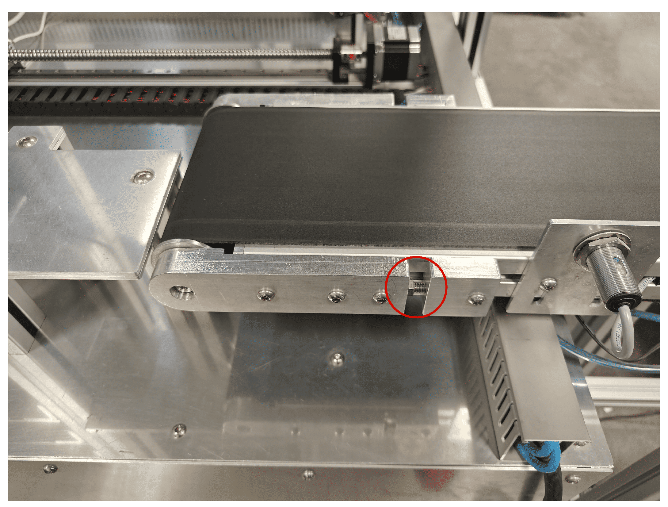
The failures analyzed in the conveyor belt were low tension and friction. To reduce tension, the belt tensioner is adjusted, as it is indicated with the red circle in Figure 2. For the second failure, an object is placed between the belt support structure and the belt, creating friction that affects its movement.

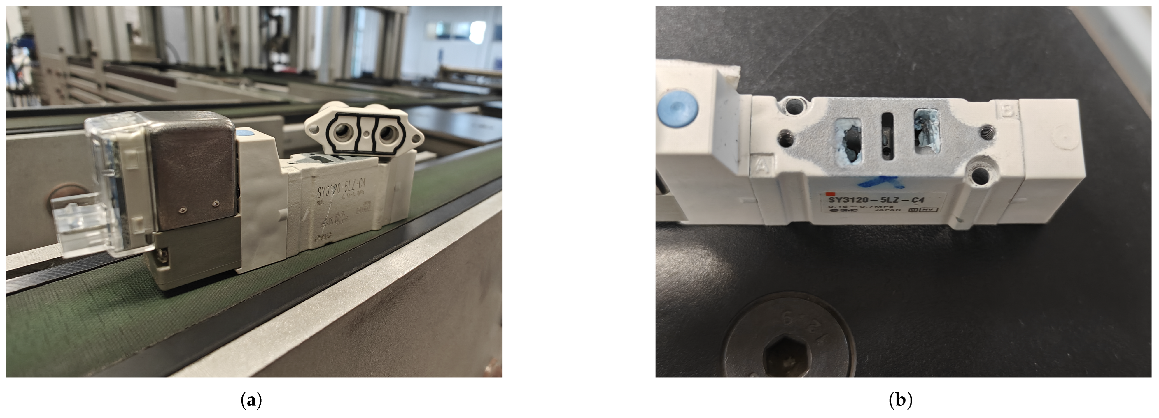
In the case of the valve, the evaluated failures were worn valve, packing leakage, hose leakage, and blocked pathways. For the worn valve or valve wear failure, the valve originally installed in the module was monitored and compared to a completely new solenoid valve, which was considered the optimal condition or proper functioning of the equipment. Subsequently, the packing was removed from the solenoid valve to induce leakage due to the lack of packing (see Figure 3a), while for the hose leakage, a cut was made to the hose. Finally, epoxy putty was applied (see Figure 3b) to simulate dirt or dust, which commonly block the pathways of the solenoid valve.

On the other hand, the following failures were induced in the cylinder: shortage of covers, lack of suction, and broken hose. It can be observed that some of these failures are not inherent to the component itself but rather are related to the process and function the cylinder serves, such as the shortage of covers in the reservoir or the lack of suction.

2.3. Sensors

Some of the most commonly used parameters for monitoring equipment conditions include vibration, temperature, current, and sound [2]. Therefore, it was necessary to find cost-effective alternatives to measure these parameters, as the equipment typically used in predictive maintenance is very expensive. For this reason, the following sensors were selected:

• MPU6050: A six-axis accelerometer and gyroscope sensor used to measure linear and angular acceleration. It uses the I2C communication protocol to connect with Arduino boards.
• SCT-013-030: The SCT-013-030 current sensor is a non-invasive device that allows the measurement of alternating current intensity up to 30 Amperes. An ADS1115 analog-to-digital converter (ADC) is used to amplify and convert the analog signal from the SCT-013-030 into a digital signal, which can be read by the Arduino through the I2C protocol.
• LM35: The LM35 is a temperature sensor that provides a linear analog output with a slope of 10 mV/ºC and allows temperature measurements in the range of −55 °C to 150 °C. This output can be directly read by the Arduino’s ADC. Two of these sensors are used: one to monitor the equipment temperature and another, placed away from the system, to measure the ambient temperature.
• KY-038: The KY-038 sound sensor module consists of a microphone that detects sound frequency variations and outputs either an analog or digital value.

In the case of the pneumatic components, the current sensor was replaced by a differential pressure sensor MPX5700DP:

• MPX5700DP: This is a piezoelectric differential pressure sensor that detects the pressure difference between two points and converts this difference into a proportional electrical signal. It is designed to measure differential pressures within a specific range, from 0 to 700 kPa.

2.4. Development Board

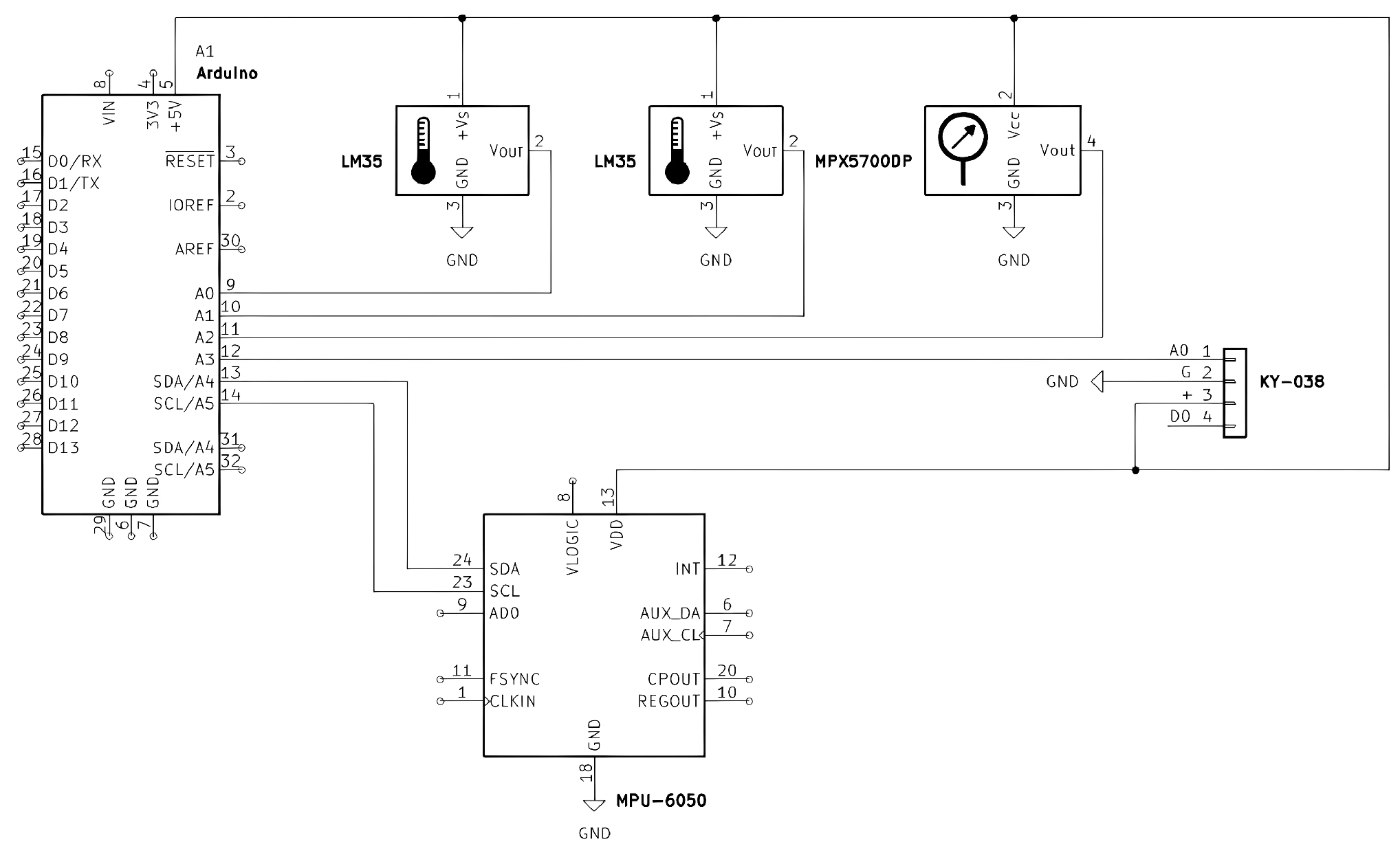
Due to its versatility and wide compatibility with a variety of sensors, Arduino is an excellent option, considering the range of sensors used in this project. Additionally, it is an affordable alternative recommended for small and medium-sized projects, as mentioned in [18]. Therefore, the Arduino Due was selected to carry out this project. Figure 4 shows the data acquisition system used to monitor the pneumatic components. In the case of the conveyor system, the MPX5700DP sensor is replaced by the SCT-013-030 current sensor.

2.5. Data Acquisition

The Arduino Due was programmed to continuously acquire data from the sensors in real time. A sampling frequency of 120 Hz was established, the minimum required to capture the electrical signal according to the Nyquist theorem, in order to capture rapid changes in the operational conditions of the conveyor belt, the valve, and the cylinder, thus ensuring accuracy in the measurement of vibration, current, and sound.

In this data acquisition project, the data are transmitted from Arduino via serial communication and received in Python 3.9.13, where it is captured in real time. Once monitoring is complete, the data are exported and stored in “.xlsx” format for further analysis and processing.

The system is configured to monitor the conveyor belt motor, from the first analyzed system Figure 1a, over two complete cycles, corresponding to a total duration of 2.4 s. During each cycle, data is collected and saved for subsequent analysis. After completing two cycles, the monitoring automatically restarts to continue recording the motor signals. In the case of the pneumatic components, from second system Figure 1b, the monitoring period extends to 5 s, which corresponds to the full operating cycle of the cap placement station. Due to this longer cycle time, the number of samples obtained from pneumatic components is lower compared to the conveyor belt system. For the conveyor belt, 500 samples were obtained for each failure and the normal condition of the equipment, totaling 1500 samples. For the valve, 300 samples were recorded for each component state, and for the cylinder, 150 samples were recorded, totaling 1500 and 600, respectively.

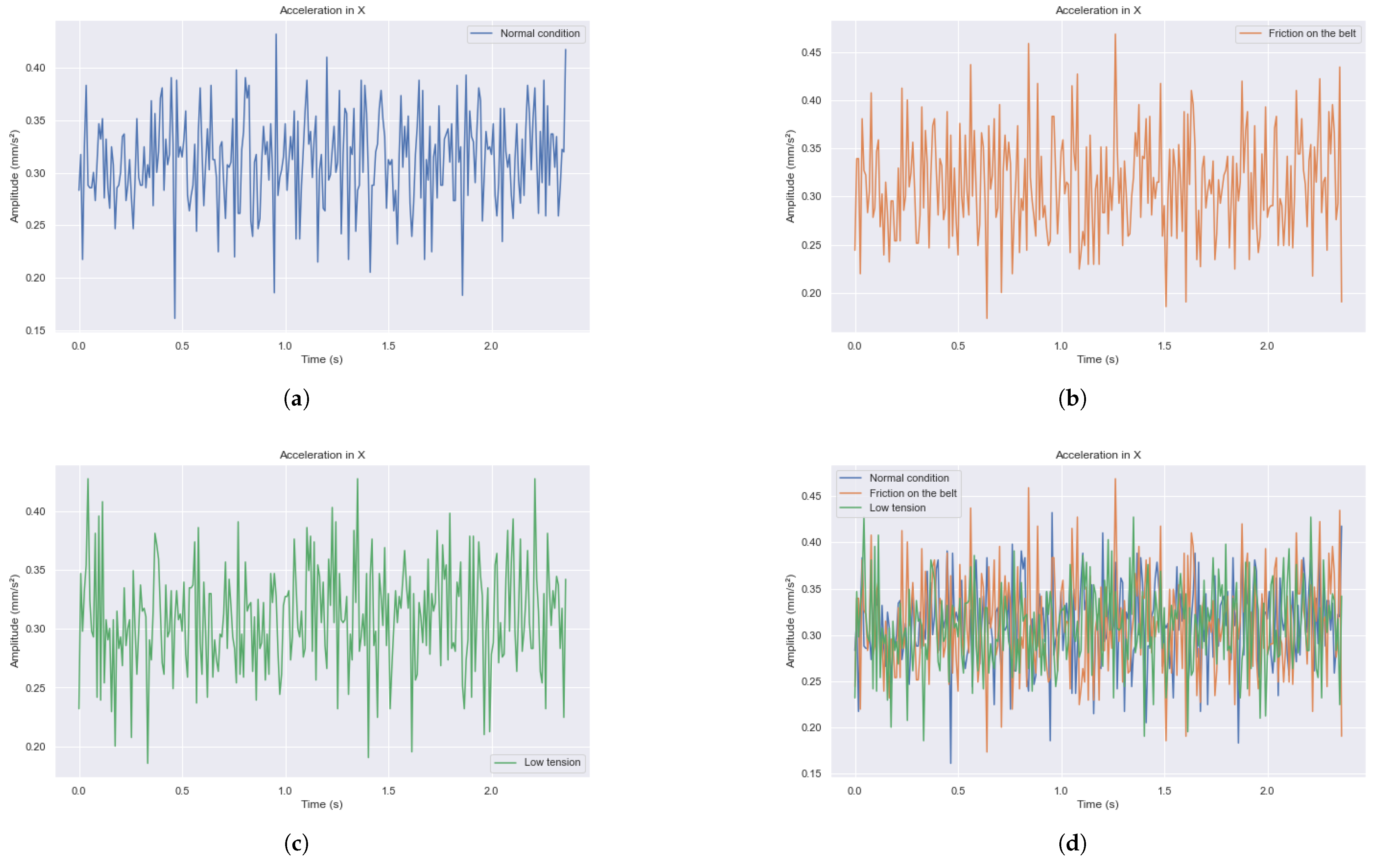
Figure 5 shows the records obtained directly from the vibration sensor during the unprocessed measurement process. These graphs represent the temporal evolution of the acquired data, providing a clear and accurate visualization of the raw measurements recorded by the sensor during each capture cycle. In Figure 5a–c, the signals in the time domain of the acceleration measured by the accelerometer along the X-axis for each of the conveyor belt failures are shown in isolation. In Figure 5d, these signals are overlaid, clearly highlighting the differences in the signals depending on the failure being analyzed.

2.6. Data Processing

For data processing, fast Fourier transform (FFT) is applied to each of the signals to obtain the signals in the frequency domain. To classify the conveyor belt failures, various characteristics recommended in [5,14,19] are extracted. In both the time and frequency domains, the following features were extracted:

• Average;
• Root mean square (RMS);
• Standard deviation;
• Skewness;
• Kurtosis;
• Shape factor;
• Crest factor;
• Impulse factor.

Once all these features are extracted, dimensionality reduction is performed using the backward elimination and principal component analysis (PCA) methods. For backward elimination, a threshold value of $\alpha =0.05$ is set. For PCA, a minimum variance ratio of 0.95 is proposed.

After feature selection, a numerical value is assigned to each of the states or failures evaluated for data processing and result display, and they are placed in a separate array from the features.

For the conveyor belt,

0.

Normal condition (no failure);

1.

Friction on the belt;

2.

Low tension.

For the valve,

0.

New valve;

1.

Leakage due to lack of packing;

2.

Leakage due to broken hose;

3.

Obstruction in pathways;

4.

Worn valve.

Finally, for the cylinder,

0.

Normal condition;

1.

Leakage due to broken hose;

2.

Missing covers in the reservoir;

3.

Lack of suction in the suction cup.

It is also necessary to normalize the extracted features, a process carried out using the StandardScaler tool in Python.

At this point, the dataset is divided into two subsets: one for training the model and for evaluating its performance. An 80:20 ratio is used (80% of the data are used to train the models, while the remaining 20% are used to evaluate the model’s ability to generalize its predictions).

2.7. Algorithms

Once the data processing is completed, the next step is the creation of the models. The choice of algorithms was based on [20], which identifies the most commonly used algorithms in the literature by researchers. The selected algorithms for this work are as follows:

• SVM,
• Decision trees,
• Ensemble models (random forest, boosting, stacking),
• KNN,
• MLP.

2.7.1. SVM

SVM consists of finding a hyperplane y of following the form:

$$y=W^{T}x+b=\sum _{i=1}^N{W}_i{x}_i+b=0$$

(1)

where W is the normal or orthogonal vector to the hyperplane, indicating the direction perpendicular to it; x is the feature vector or input vector; N represents the number of variables or features in the input vector x; and b is the bias of the hyperplane, referring to the distance between the origin and the hyperplane in relation to its orientation defined by W. This is executed in such a way that the classes are separated optimally, meaning that it involves finding the hyperplane with the largest possible margin. A hyperplane is a subspace that has a lower dimension than the space in which it is contained, while the margin is the distance between the hyperplane and the support vectors, which are the closest points of different classes to each other [21,22,23].

2.7.2. Decision Tree

Decision trees are called as such due to their tree-like structure, similar to a flowchart. It consists of internal decision nodes and terminal leaves. Each decision node performs a test with discrete results to label the branches. The process starts at the root node and repeats until it reaches a leaf node, where the determined value constitutes the output; therefore, decision trees can be seen as a series of “if-then” conditions [21,24]. A node is considered pure when all the samples it contains belong to the same class. The decision tree evaluates which attribute best divides the data based on an impurity criterion, such as entropy:

$$I_m=-\sum _{j=1}^N{\displaystyle \frac{N_{mj}}{N_m}}\sum _{i=1}^k{p}_{mj}^{i}lo{g}_2{p}_{mj}^i$$

(2)

where $I_m$ is the impurity of node m, $N_m$ is the total number of examples in node m, $N_{mj}$ is the number of examples in category j in node m, N is the number of categories of the categorical feature being used to split node m, and $p_{mj}^i$ is the probability that an example from node m belongs to class i in category j [21].

2.7.3. Ensemble Methods

Combined models, also known as model ensembles, are highly effective approaches in machine learning, generally outperforming the performance of individual models. They are based on a statistical theory that states that averaging measurements can lead to a more reliable and stable estimate, as it reduces the effect of random fluctuations in individual measurements. By combining several models, the strengths of each algorithm are leveraged while compensating for their weaknesses. Additionally, they tend to be more robust and stable compared to using a single algorithm, but they often involve higher computational cost and complexity. Some of the most popular ensemble methods are bagging, boosting, and stacking, as well as Random Forest [24,25].

2.7.4. K-Nearest Neighbors

KNN classifies unlabeled objects by examining the classes of the K nearest objects in the training set. The label for an unlabeled object is determined based on the most frequent class among these nearest neighbors [22]. First, the algorithm calculates the distance between the unlabeled object and the training objects to identify the closest neighbors. A distance metric, such as Euclidean distance, is used to define the level of proximity [24] and [26]:

$$D(X,Y)=\sqrt{{\displaystyle \sum _{i=1}^N}{(x_i-y_i)}^2}$$

(3)

Then, it assigns the most common class among these neighbors as the label for the unlabeled object.

2.7.5. Multi-Layer Perceptron

An MLP is a class of artificial neural network with forward propagation and more than one layer. It consists of an input layer, one or more hidden layers, and an output layer, where every neuron in each layer is connected to a neuron in the next layer, and there are no connections between neurons within the same layer. The number of neurons in the input layer is equal to the number of features in the input data, and the number of nodes in the output layer is equal to the number of categories in the output data. The output of the neural model can be obtained using the following equation:

$$y=f\left(W^{T}x\right)=f({\displaystyle \sum _{i=1}^N}{w}_i{x}_i+b)$$

(4)

where f is the activation function, x is the input vector, N is the number of neurons, W is the weight vector, and b is the bias vector. Generally, the activation functions used are the sigmoid function and the tanh function for the hidden layers and the Softmax function for the output layer [27,28,29,30].

2.7.6. Cross-Validation

Firstly, a cross-validation process was conducted to select the hyperparameters that yield the best results. The process began with SVM, utilizing the radial basis function (RBF) kernel, as it enables the modeling of nonlinear and complex relationships and is less prone to overfitting. The values for $\gamma$ and the regularization parameter C were determined through cross-validation by combining various values: $2^{\mathrm{-15}}$, $2^{\mathrm{-13}}$, …, 2, $2^3$ for $\gamma$; and $2^{\mathrm{-5}}$, $2^{\mathrm{-3}}$, …, $2^{13}$, $2^{15}$ for C [31].

For the decision tree algorithm, the hyperparameters included the purity index (Gini or Entropy), the minimum number of samples per leaf (1, 2, 5), the minimum number of samples required for a node to be split (2, 5, 10), and the maximum tree depth (5, 10, 15, 20, 25, 30, 35, 40, 45, 50, None). The decision tree obtained at this point is used for the boosting and random forest algorithms, each with 40 estimators.

For the KNN algorithm, only two hyperparameters were considered: k (the number of neighbors), which varied from 1 to 41 (taking only odd values) and the distance metric (Euclidean or Manhattan).

In the case of the stacking algorithm, it takes as input the predictions from the aforementioned base models (SVM, decision tree and KNN), as well as the predictions generated by bagging (random forest) and boosting algorithms. The final classifier, responsible for making the ultimate decision, is the default classifier provided by the scikit-learn library, which is typically a logistic regression model.

Lastly, for the MLP neural networks, the parameters included the number of epochs (10, 20, 50, 100 or 200), the activation function (ReLU or Tanh), and the optimizer (SGD, RMSprop or Adam). Additionally, different numbers of neurons and layers were tested, with neuron counts of 2, 4, 8, 16, 32, 64, and 128, and the network could consist of two or three hidden layers.

2.8. Evaluation Metrics

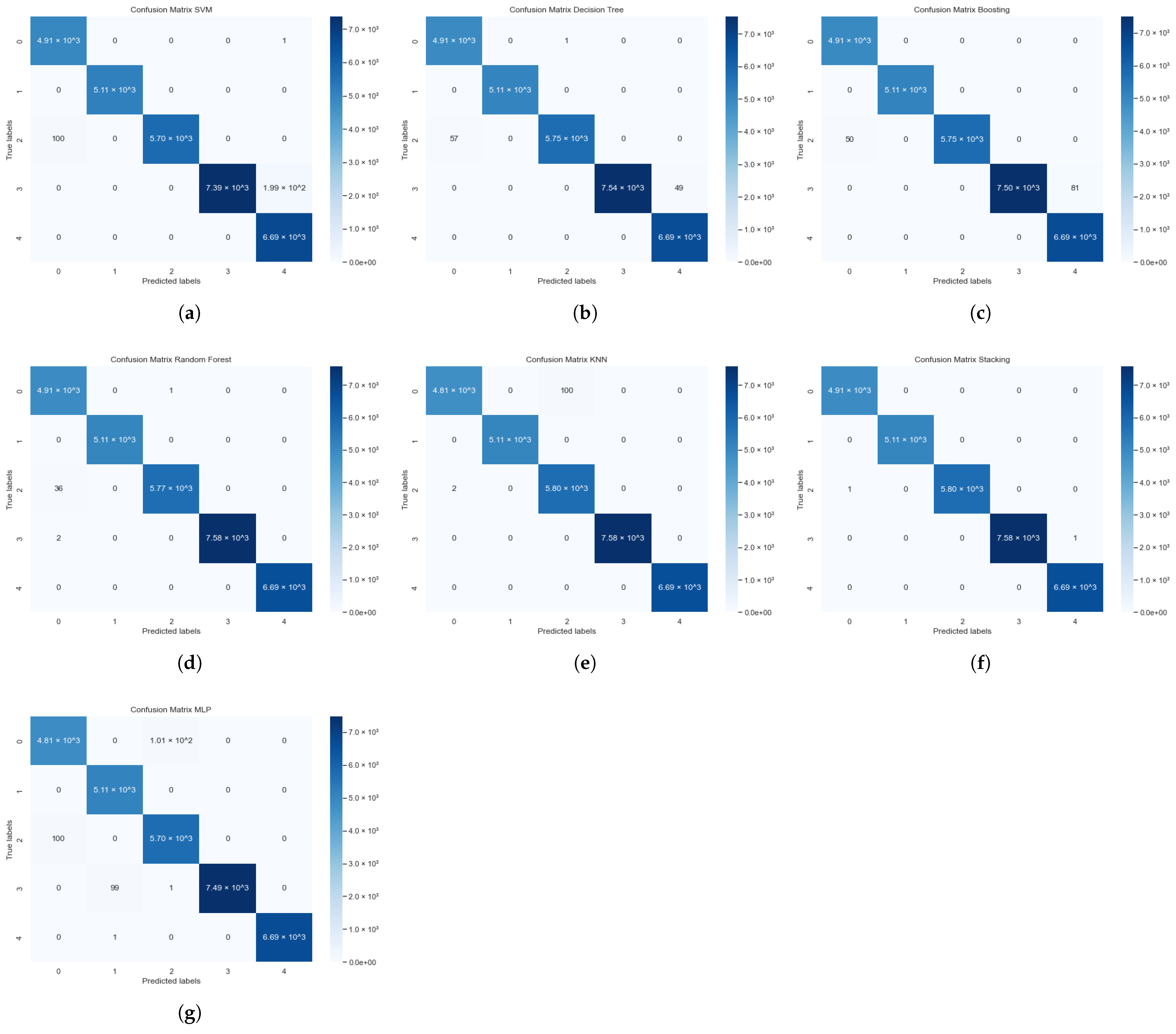
Once the hyperparameters were determined, the algorithms were trained using the training set, followed by prediction generation using the test set. These predictions were compared with the actual outputs, resulting in confusion matrices such as the ones shown in Figure 6. The confusion matrix, also known as the error matrix, is a representation that shows how a classification algorithm performs using the available data. It compares the predicted classifications with the actual classifications, where each prediction can result in one of four outcomes based on how it matches the true value [24,25]:

• True positive (TP): the output is correctly identified as positive.
• True negative (TN): the output is correctly identified as negative.
• False positive (FP): the output is incorrectly identified as positive.
• False negative (FN): the output is incorrectly identified as negative.

The ideal scenario is for the model to have zero false positives and zero false negatives.

This process was replicated 100 times in order to assess the stability of the algorithms. In each of these repetitions, the training and test sets were recalculated.

The confusion matrix itself is not a performance metric, but most performance metrics are derived from the confusion matrix and the values it contains. Rerunning the algorithm multiple times facilitates the calculation of more robust performance metrics, allowing for the averaging of these metrics to provide a more reliable assessment of the model’s efficacy. Among the key metrics utilized in model evaluation are precision, recall, F1-score, and accuracy, each of which offers a distinct insight into the model’s performance.

$$Accuracy={\displaystyle \frac{TP+TN}{TP+TN+FP+FN}}$$

(5)

$$Precision={\displaystyle \frac{TP}{TP+FP}}$$

(6)

$$Recall={\displaystyle \frac{TP}{TP+FN}}$$

(7)

$$F1=2\times {\displaystyle \frac{recall\times precision}{recall+precision}}$$

(8)

3. Results and Discussion

3.1. Performance Evaluated on the Complete Set of Samples

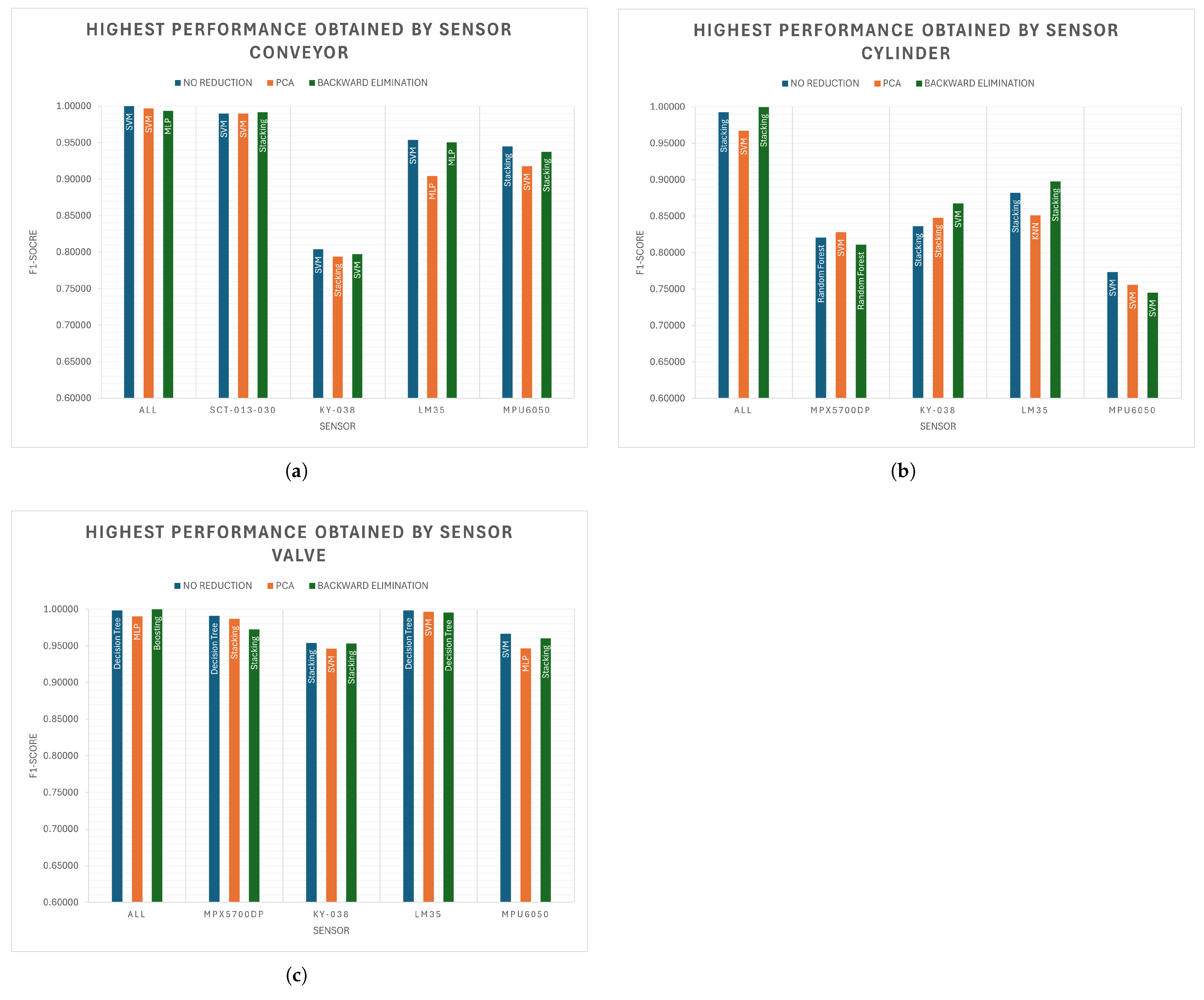
As a result of each comparison between the predicted value by the algorithm and the actual failure value, the results shown in the graphs of Figure 7 were obtained. These graphs display the F1-score value of the algorithm that yielded the best result based on the sensor monitoring the equipment and the variable reduction method used.

These results represent the best performance achieved by each of the sensors evaluated during the study. Therefore, it can be inferred that, under similar operating conditions, these specific sensors, when paired with their corresponding algorithms, may serve as viable alternatives for implementation in comparable scenarios. In the event that the system architecture or application context permits their integration, the utilization of these sensors is recommended due to their demonstrated effectiveness and reliability within the experimental framework.

It can be observed that, in general, the most favorable results were achieved through equipment monitoring using the SCT-013-030 current sensor and the MPX5700DP differential pressure sensor. These sensors provided highly accurate signals that enabled effective fault classification. Additionally, the LM35 temperature sensor also demonstrated strong performance in detecting abnormal operating conditions. Although the SCT-013-030 and MPX5700DP stand out in terms of diagnostic capability, their overall implementation cost—including hardware, installation, and signal conditioning—is notably higher compared to that of the LM35. In contrast, the LM35 offers several advantages: it is low-cost, easy to integrate, and broadly compatible with a wide range of industrial equipment. These characteristics make it a practical and scalable option for temperature-based condition monitoring, especially in resource-constrained environments or when deploying a large number of sensing points is required.

It is also worth noting that the KY-038 sound sensor, which was included in the evaluation, demonstrated poor performance in this study. Its inability to provide reliable or distinctive acoustic signals under varying operational conditions suggests that it may not be a suitable choice for fault diagnosis in industrial environments.

By counting the occurrences of each algorithm in Figure 7, it is possible to make an initial evaluation of the algorithms’ performance:

• SVM: 17;
• Stacking: 15;
• MLP: 5;
• Decision tree: 4;
• Random forest: 2;
• Boosting: 1;
• KNN: 1.

The preceding list suggests that all evaluated algorithms demonstrated, at least once, an acceptable level of performance across the various experimental configurations. This observation indicates that, in principle, any classification algorithm may be viable for industrial fault detection, provided it is properly tuned and aligned with the characteristics of the data and operational context. Moreover, it can be observed that the SVM algorithm stands out from the others due to having a higher number of occurrences. However, as mentioned previously, Figure 7 contains the best results for each specific case. Therefore, to determine which algorithm might perform better in the industry in general, it is necessary to use all the results obtained.

Table 1. Average evaluation metrics obtained by each algorithm, according to the variable reduction method employed.

Variable Reduction	Algorithm	Precision	Recall	F1-Score	Accuracy
No reduction	SVM	0.9214	0.9204	0.9202	0.9204
	Decision Tree	0.8998	0.8976	0.8971	0.8975
	Boosting	0.9069	0.9064	0.9060	0.9064
	Random Forest	0.9114	0.9108	0.9098	0.9108
	KNN	0.8943	0.8922	0.8914	0.8922
	Stacking	0.9226	0.9222	0.9218	0.9222
	MLP	0.9108	0.9103	0.9096	0.9104
PCA	SVM	0.9124	0.9109	0.9105	0.9110
	Decision Tree	0.8256	0.8177	0.8184	0.8178
	Boosting	0.8559	0.8537	0.8538	0.8537
	Random Forest	0.8693	0.8671	0.8661	0.8672
	KNN	0.8871	0.8861	0.8844	0.8863
	Stacking	0.9060	0.9051	0.9046	0.9052
	MLP	0.9007	0.9005	0.8997	0.9006
Backward elimination	SVM	0.9195	0.9172	0.9173	0.9172
	Decision Tree	0.8935	0.8895	0.8882	0.8896
	Boosting	0.9051	0.9050	0.9045	0.9050
	Random Forest	0.9028	0.9023	0.9008	0.9023
	KNN	0.8903	0.8881	0.8874	0.8883
	Stacking	0.9211	0.9205	0.9201	0.9205
	MLP	0.9090	0.9090	0.9082	0.9091

illustrates the mean values of the evaluation metrics for each algorithm, segmented according to the variable reduction technique applied. In contrast,

Table 2. Overall average of the evaluation metrics.

Algorithm	Precision	Recall	F1-Score	Accuracy
SVM	0.9178	0.9161	0.9160	0.9162
Decision Tree	0.8729	0.8683	0.8679	0.8683
Boosting	0.8893	0.8883	0.8881	0.8883
Random Forest	0.8945	0.8934	0.8922	0.8935
KNN	0.8906	0.8888	0.8877	0.8889
Stacking	0.9166	0.9159	0.9155	0.9160
MLP	0.9068	0.9066	0.9058	0.9067

consolidates the overall mean values of the evaluation metrics across all algorithms.

Table 1 suggest that, in this particular case, dimensionality reduction is not essential. Overall, the application of either PCA or backward elimination did not lead to significant improvements in classification performance. In fact, in several instances, the use of these techniques resulted in a slight degradation in accuracy, likely due to the removal or transformation of features that, while subtle, contained critical information for fault detection. These findings underscore the importance of carefully weighing the trade-offs involved in feature reduction, particularly when working with datasets that already comprise a manageable and relevant set of input variables. Nonetheless, in scenarios where dimensionality reduction is necessary—due to computational constraints, real-time processing demands, or limited data acquisition—certain algorithm-method combinations demonstrated more stable behavior. Specifically, SVM paired with PCA maintained consistent performance, suggesting that SVM can effectively utilize the orthogonalized feature space created by PCA. Similarly, boosting combined with backward elimination showed competitive results, indicating a degree of robustness to feature selection.

The values in Table 1 are averaged to obtain the overall results across all dimensionality reduction methods, which are shown in Table 2.

Finally, considering that the dataset used in this study maintains a balanced distribution among its categories, it is sufficient to rely on the accuracy metric as a primary indicator of algorithmic performance. In datasets where each class is equally represented, accuracy provides a reliable measure of the model’s ability to correctly classify instances across all categories. Therefore, by simply ordering the results in Table 2 from highest to lowest accuracy, it is possible to determine which algorithms achieved the best performance within the analyzed systems.

• SVM;
• Stacking;
• MLP;
• Random forest;
• Boosting;
• KNN;
• Decision tree.

These results are very similar to those obtained in the previous list created using Figure 7, considering the SVM algorithm to be the one that is best adapted to conditions similar to those that may arise in the industry. The algorithms that appear at the top of the performance ranking demonstrated superior performance when applied to datasets characterized by a balanced distribution across all categories. This indicates that these algorithms are particularly well-suited for scenarios in which the dataset contains an equal or near-equal proportion of instances for each class, thereby minimizing potential bias and enhancing the overall accuracy and generalization capability of the classification process.

3.2. Performance Evaluated on 5% of the Complete Set of Fault Samples

However, in a real-world factory environment, equipment is expected to operate correctly most of the time; therefore, a significant portion of the collected data naturally correspond to normal operating conditions. Furthermore, the practical objective in industrial settings is to enable the diagnosis of failures over extended periods while requiring minimal training data. In light of this, the same classification process was repeated using only 5% of the available failure-related data. Specifically, for the conveyor system, where the total dataset for failures comprises 1000 samples (500 for each type of failure), only 50 samples were utilized in this scenario. Additionally, the data split was adjusted to reflect a more realistic application context, allocating 20% of the data for training and the remaining 80% for testing. The results obtained under these conditions are presented below (

Table 3. Average of the performance metrics of each algorithm.

Algorithm	Precision	Recall	F1-Score	Accuracy
SVM	0.69586	0.67080	0.66838	0.93307
Decision Tree	0.60049	0.61124	0.59169	0.90873
Boosting	0.65003	0.60764	0.60464	0.90277
Random Forest	0.63917	0.56525	0.57384	0.92239
KNN	0.73177	0.64755	0.65529	0.92448
Stacking	0.63104	0.58806	0.59048	0.92528
MLP	0.67049	0.63971	0.63572	0.92561

).

Once again, the algorithms will be ranked according to their effectiveness; however, in this case, the evaluation will be based on the F1-score rather than accuracy. This decision is motivated by the fact that the dataset used in this phase does not exhibit a proportional distribution among its categories. Under such conditions, accuracy alone may offer a misleading representation of model performance, particularly in the presence of class imbalance. The F1-score, which considers both precision and recall, provides a more balanced and informative metric for assessing classification outcomes in imbalanced datasets.

• SVM;
• KNN;
• MLP;
• Boosting;
• Decision tree;
• Stacking;
• Random forest.

The results obtained in this section differ from those presented previously. Consequently, the experiment was repeated with varying proportions of samples representing normal operating conditions and failures. Specifically, all available samples corresponding to good condition were retained, while the proportion of failure samples was systematically reduced. The selected percentages of failure data included 100%, 80%, 60%, 40%, 20%, 10%, and 5%, allowing for a detailed analysis of how class imbalance affects the performance of the classification algorithms. The results obtained are shown in the graph of Figure 8.

As can be seen in Figure 8, the results obtained in this section remain consistent with those from the previous analysis as long as the proportion of failure samples relative to good condition samples does not fall below 20%. Notably, the top three algorithms identified earlier continue to demonstrate superior performance within this range. However, once the failure data are reduced below this threshold, a significant drop in performance is observed. This degradation appears to be particularly pronounced in ensemble-based methods. It is hypothesized that, under conditions of extreme class imbalance, the diversity of errors produced by individual models within the ensemble becomes so pronounced that, rather than correcting one another through aggregation, these errors are compounded. As a result, the ensemble mechanism fails to achieve its intended robustness and instead amplifies misclassifications.

The results indicate that SVM consistently exhibited superior performance, regardless of the ratio between failure and normal condition samples. SVM is a good option due to its simplicity and ease of application, its straightforward implementation and strong performance in classification tasks make it an ideal choice for fault diagnosis in industrial systems. Algorithm MLP similarly demonstrated high generalization capability across different degrees of class imbalance, suggesting its potential suitability for real-world industrial scenarios, which often feature a limited number of failure events. In addition to SVM and MLP, which consistently demonstrated robust performance across varying class distributions, some good options can be identified depending on the ratio of failure to normal condition samples. The stacking method performs well when the dataset is balanced. This suggests that stacking is particularly well-suited for scenarios where class distribution is not skewed. On the other hand, under conditions of severe class imbalance, where failure instances are significantly outnumbered, KNN emerges as a reliable alternative, showing strong capability in detecting minority class instances. These findings highlight that, beyond raw performance metrics, the choice of algorithm should take into account its sensitivity to data distribution, especially in industrial settings where failure events are inherently rare.

4. Conclusions

In this work, different machine learning algorithms were compared, applied to the fault diagnosis of various components, with the goal of determining which of these provides the best overall results in the industrial environment.

In conclusion, while all evaluated algorithms are potentially viable for industrial fault detection, SVM and MLP stand out for their consistent and robust performance across various class distributions. Stacking is particularly effective in balanced datasets, whereas KNN performs well under severe class imbalance. These insights suggest that selecting a machine learning algorithm for fault diagnosis should consider not only performance but also the nature of the data and the operational context, with special attention to class imbalance—an inherent characteristic of most industrial scenarios.

On the other hand, while the SCT-013-030 and MPX5700DP sensors achieved the highest diagnostic performance, their high implementation cost may limit their use in large-scale or budget-constrained applications. The LM35 temperature sensor, by contrast, presents a cost-effective and scalable alternative for condition monitoring, combining reasonable diagnostic capability with ease of deployment. The KY-038 sound sensor, however, proved inadequate for industrial fault detection due to its unreliable performance, indicating that it is not a viable option for this context.

Finally, dimensionality reduction techniques such as PCA and backward elimination did not significantly enhance classification accuracy in this study and, in some cases, even slightly reduced it. This outcome highlights the importance of retaining critical input features in industrial fault diagnosis, where subtle data patterns may carry essential diagnostic information. However, in contexts where feature reduction is unavoidable, pairing SVM with PCA or boosting with backward elimination may offer more stable performance, making them suitable choices under constrained computational or data acquisition conditions.

Future work will focus on exploring a broader range of deep learning algorithms to compare their performance in fault diagnosis. Additionally, the proposed approach will be applied to a wider variety of components, further extending its applicability and robustness in real-world industrial environments.