Abstract
In distributed microgrid systems, inverters serve as the core components when distributed generation (DG) modules are integrated into the grid. Traditional inverters typically employ droop control; however, they lack damping and inertia mechanisms. Consequently, fluctuations in the grid frequency and voltage occur when system loads change, leading to a suboptimal power distribution. To address these limitations, this paper introduces an adaptive strategy into conventional droop control. Based on an adaptive algorithm, the real and reactive power are dynamically computed. Through coordinate transformation, decoupled control, and adaptive frequency compensation, the inverter’s output frequency and voltage are effectively regulated. By adjusting the reference current in a dual-loop control scheme, the active and reactive power distribution is optimized. Additionally, an improved adaptive algorithm is developed to compute the inverter’s AC frequency compensation, enabling the self-adaptive adjustment of the PI controller’s output. This facilitates frequency compensation in droop control, ensuring that the inverter’s output current and voltage remain synchronized with the grid phase, thereby enhancing grid stability during connection. Finally, the feasibility of the proposed algorithm is validated through Simulink simulations.
1. Introduction
With the rapid development of social and economic development, the demand for electricity is increasing, but the problem of environmental pollution from conventional power generation is also more serious. Moreover, conventional power generation methods have led to significant environmental pollution [1,2,3,4,5]. As the global awareness of environmental protection grows, microgrid technology based on renewable energy sources such as solar and wind power has gained increasing attention as a means to mitigate the environmental impacts of traditional energy generation. Since the introduction of distributed generation (DG) microgrid technology [6,7], its unique advantages have facilitated its rapid development and integration into power systems, gradually making it an essential component of modern electrical grids [8,9].
Distributed power sources convert renewable energy, such as wind and solar power, into electrical energy, which is then transformed into grid-compatible alternating current (AC) through inverters composed of power electronic components. As the core unit responsible for DC-AC conversion in distributed power systems, the inverter plays a critical role in ensuring high-quality power generation. Its control performance is essential for maintaining voltage and frequency stability, achieving optimal power distribution, and ensuring the safe and reliable operation of the microgrid [10,11,12,13].
When distributed power sources operate in parallel, traditional droop control can be employed to regulate the system voltage and frequency by simulating the droop characteristics of conventional generators [14,15,16,17,18]. This method enables the decoupled control of active and reactive power with respect to voltage and frequency, facilitating a balanced distribution of load power among the various distributed generation modules while maintaining stable system voltage and frequency. However, due to factors such as differences in line impedance, reactance, voltage magnitude, and structural variations, power coupling issues may arise [19,20,21]. When load fluctuations occur, conventional P-V/Q-F droop control may fail to promptly adjust the power distribution, potentially leading to significant reactive power circulation between micro-sources and fluctuations in the output voltage and current of the inverter system [22].
In this paper, the main research work used an adaptive adjustment mechanism combined with the improved Fal function. The output voltage–frequency compensation value of the inverter is dynamically adjusted according to the droop equation through the control of the phase difference between the inverter output voltage synthesis vector and the grid voltage synthesis vector by coordinate transformation and adaptive frequency compensation. The reference voltage is calculated according to the compensated frequency, the output of the inverter is regulated by the double closed-loop control of the voltage outer loop and current inner loop, and the system has good control accuracy. Adaptive controllers enable the fast and accurate modulation of the inverter output voltage and phase during sudden load changes. The system has a good dynamic response speed and stronger anti-interference ability.
2. Droop Control
The frequency of a power system directly reflects the active power balance state of the system. When the active power is greater than the load, the frequency increases; conversely, the frequency decreases. Fluctuations in frequency can lead to an unbalanced, suboptimal power distribution. When the voltage drops, the system may need to increase the reactive power to maintain the voltage level, while when the voltage rises, it may need to decrease the reactive power.
During power system fluctuations, primary frequency regulation is often employed to suppress deviations. Droop control serves as a means of simulating this primary frequency regulation in power systems [23,24,25]. By replicating the droop characteristic curve of a conventional generator, droop control regulates the inverter’s output voltage magnitude and frequency, ensuring the proper distribution of output power while maintaining the voltage and frequency stability of the microgrid system.
When the impedance of high-voltage transmission lines is predominantly inductive, the system’s output impedance can be approximated as purely inductive. Under such conditions, when the system load fluctuates [26,27], the linearized relationship between active power and frequency, as well as reactive power and voltage, can be described as shown in Figure 1 and Figure 2.
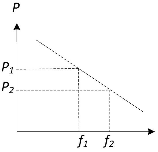
Figure 1.
Frequency/Active power curve.

Figure 2.
Voltage/Reactive power curve.
Its relational expression is as follows:
The parameters and represent the droop control coefficients for power regulation. The variables P′, Q′, U′, and ω′ denote the rated active power, rated reactive power, rated voltage, and rated frequency of the inverter, respectively. Meanwhile, P and Q correspond to the actual active and reactive power outputs of the inverter.
3. Mathematical Modeling of Shunt Inverters for Microgrids
3.1. Inverter Main Circuit Structure
This study focuses on a three-phase voltage-source inverter, where the DC side of the inverter is equivalently modeled as a voltage source, and the output is represented as a controlled voltage source. The main circuit topology consists of a three-phase full-bridge configuration, with an LC filter at the output stage. In this system, uoa, uob, and uoc represent the capacitor voltages, while ioa, iob, and ioc denote the inductor currents. The parameter ZL corresponds to the load impedance. The schematic diagram of the three-phase inverter main circuit is illustrated in Figure 3.
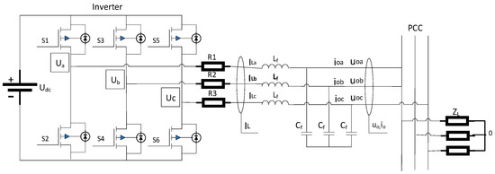
Figure 3.
Main parallel circuit structure of the voltage source-type three-phase inverter.
The three-phase inverter outputs are ua, ub, and uc, with a phase difference of 120°, where Um represents the amplitude of the synthesized voltage vector. The spatially synthesized vector in the stationary three-phase coordinate system is illustrated in Figure 4. The voltage and current calculation formulas are given in Equation (2), where ω is the fundamental frequency of the power source.
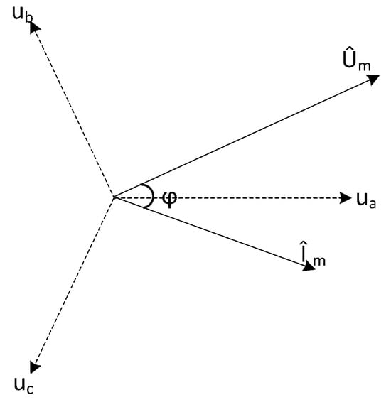
Figure 4.
Space vector diagram of three-phase stationary coordinate system.
The six power switches in the three-phase inverter bridge are driven by sinusoidal pulse-width modulation (SPWM) signals, which are generated through the carrier-based modulation of a sinusoidal reference signal. A set of three sinusoidal waveforms, each phase-shifted by 120°, is compared with a triangular carrier wave to produce the control signals required for switching. These control signals regulate the switching states of the six insulated gate bipolar transistors (IGBTs) in the upper and lower bridge arms, ensuring the generation of a three-phase AC output at the load terminal with the same frequency as the modulation wave. The output of the three-phase inverter is connected through the point of common coupling (PCC) to supply power to the load impedance ZL.
3.2. Vector Space Coordinate Transformation
In a three-phase power grid, the voltage and current of each phase vary sinusoidally over time. Directly analyzing these time-dependent waveforms can be complex. To simplify the calculations, the Clark and Park transformations are introduced. These transformations first convert the three-phase stationary coordinate system into a two-phase α-β stationary coordinate system and subsequently into a two-phase dq rotating coordinate system, where the variables become time-invariant in a steady-state condition. This facilitates analysis and control. The original three-phase AC voltage or current waveforms can then be reconstructed using the inverse dq/abc transformation.
3.3. Three-Phase Stationary Coordinate System to a Two-Phase Stationary Coordinate System
Transform the abc three-phase coordinate system into α-β two-phase stationary coordinate system by Clark transformation, realizing the abc/dq transform.
The Clark transformation leads to Equation (3):
The transformation matrix C3/2 is denoted as follows:
3.4. Two-Phase Stationary Coordinat System to Two-Phase Rotating Coordinate System
Convert the AC quantities in the two-phase stationary coordinate system to DC quantities in the dq two-phase rotating coordinate system for analysis.
The iα, iβ, id, and iq relational equation is as follows:
Expressing it in matrix form yields the following:
The transformation matrix Cabc-dq is as follows:
The three-phase capacitive voltages and inductive currents uoa, uob, uoc, ioa, iob, and ioc are transformed to the corresponding dq-axis components ud, uq, id, and iq, by the abc/dq transform. The equations are expressed as follows:
Inversion of the matrix Equation (8) can obtain the inverse transformation of a two-phase rotating coordinate system to a three-phase stationary coordinate, and the equation is expressed as follows:
4. Voltage and Current Double Closed-Loop Control
4.1. Modeling of the Dual Closed-Loop Inverter Control System
The active power P and reactive power Q are computed using Equation (10). The voltage loop parameters, including the voltage Um and frequency ω, are determined based on the droop equation (Equation (1)). After adaptive PI frequency compensation, the adjusted frequency ω* is obtained. The adaptive PI controller is designed with an improved Fal function structure to enhance performance. Using the compensated frequency, the voltage and current in the stationary reference frame are computed through Equation (2). These values are then transformed into the reference voltages uod,q∗ in the dq coordinate system. The reference voltages, along with the feedback voltages uod,q, serve as inputs to the voltage control loop, which outputs the reference current iLd,q∗ for the inner current control loop.
The reference current iLd,q*, together with the feedback inductor current iLd,q, act as the inputs to the inner current control loop, which generates the control signals iod,q in the dq coordinate system. These signals are then converted to the three-phase coordinate system values ioa,b,c through the inverse dq/abc transformation. The resulting three-phase current values are fed into the space vector pulse-width modulation (SVPWM) module, which generates six PWM duty cycle signals. These signals are used as input parameters for the inverter, controlling the switching states of the six power transistors in the three-phase inverter bridge. As a result, the inverter output is precisely regulated.
The system assumes that the equivalent output impedance of the inverter is designed as a purely inductive line, omitting the resistive component, with the impedance angle ∅n = 90°; inverter output with and LC filter; an assumption that the switching devices (e.g., IGBTs and MOSFETs) in the inverter are in ideal switching; and the assumptions that the voltage of the grid is stable and the frequency is constant. The overall block diagram of the dual-loop control system for the inverter is illustrated in Figure 5.

Figure 5.
Block diagram of the inverter dual closed-loop control system.
The computational complexity of the inverter current–voltage dual closed-loop control system mainly depends on the type of control algorithm, sampling frequency, controller structure, the performance of the implementation hardware platform, etc. The main computational tasks within each control cycle include error calculations, PI operations, coordinate transformation, and PWM modulation calculations.
The algorithm has a low computational complexity, which is suitable for systems with high real-time requirements.
Compared to other new technologies, such as fractional order PI prediction with a sliding mode, variable structure, double closed-loop control strategy, combined fractional order PI control, and predictive function control, the structure also includes a voltage outer loop and a current inner loop. The main computational tasks within each control cycle include fractional order calculus operations, predictive modelling calculations, algorithmic optimization calculations, and sliding mode control calculations
Algorithms have higher computational complexity and require higher processor performance.
The control strategy for the dual closed-loop control system relies on an accurate system model, including filter parameters, load characteristics, etc. Inaccurate modelling can also lead to degraded control performance. Moreover, when a sudden nonlinear load changes, the dual closed-loop control strategy may not be able to cope very well.
Table 1 gives a comparison of several control algorithms.

Table 1.
Algorithm comparison.
4.2. Adaptive PI Frequency Compensation Control
In conventional droop control, the inverter output frequency varies with power changes, leading to a phase difference between the output voltage and the grid voltage. This phase mismatch can result in significant inrush currents during grid connection. The grid voltage vector Ê rotates in space at a constant angular velocity ω = 2πf, where f is the fundamental grid frequency (50 Hz). To mitigate this issue, frequency compensation is applied before grid synchronization, ensuring that the inverter output voltage remains in phase with the grid voltage.
The grid voltage components ea/eb/ec are transformed into the dq coordinate system, which rotates synchronously with the inverter output voltage. The angular velocity of this rotating dq frame is determined based on the frequency derived from the droop control mechanism, ensuring that the dq frame remains synchronized with the synthesized voltage vector Û of the inverter output. To achieve phase alignment, the phase angle of the grid voltage vector Ê is controlled such that φ = 0, ensuring that the q-axis component of Ê is zero. As a result, the grid voltage vector aligns with the d-axis of the rotating dq coordinate system. A schematic representation of the vector coordinate transformation is illustrated in Figure 6.
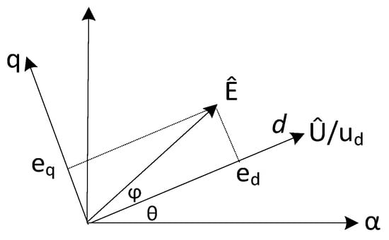
Figure 6.
Vector diagram of grid voltage synthesis.
When the q-axis component of the grid voltage vector Ê is greater than zero, it indicates that Ê leads the d-axis in phase. In this case, the angular velocity ω of the rotating dq coordinate system should be increased. Conversely, when the q-axis component of Ê is less than zero, indicating that Ê lags behind the d-axis, and ω should be reduced. The rotating dq coordinate system remains synchronized with the synthesized voltage vector of the inverter output, and ω is equivalent to the angular frequency of the three-phase AC voltage output by the inverter.
To achieve precise synchronization, the q-axis component of the grid voltage vector Ê is controlled to be zero, and an adaptive PI controller is employed to adjust the parameters dynamically, ensuring effective frequency compensation for droop control. Simultaneously, by regulating the coordinate system rotation to control the phase angle φ, the reference currents id∗ and iq∗ are allocated to manage the active and reactive power distribution of the inverter. When the q-axis current component iq is zero, the inverter exclusively outputs active power. The overall control framework is illustrated in Figure 7.
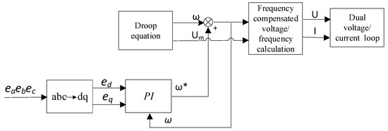
Figure 7.
PI adaptive frequency compensation control block diagram.
The adaptive PI controller integrates the proportional–integral (PI) regulation of a conventional PI controller with the Fal function, forming an optimized self-tuning parameter mechanism. This enhances the system’s rapid response and disturbance rejection capability under large-scale perturbations. The controller structure, as illustrated in Figure 7 consists of a nonlinear PI controller and a differential tracker. The nonlinear PI controller is employed to regulate the error between the actual and reference voltage values, while the differential tracker facilitates rapid phase tracking and an adjustment of the inverter output voltage. The tracking differentiator (TD) receives the q-axis component eq of the grid voltage vector Ê as its input signal, enabling real-time tracking of the q-axis component while enhancing the effectiveness of the differential signal. This ensures fast and overshoot-free tracking of eq. As the error varies, the nonlinear PI controller dynamically adjusts its PI parameters through self-tuning mechanisms. The structure of the nonlinear adaptive PI controller is depicted in Figure 8.
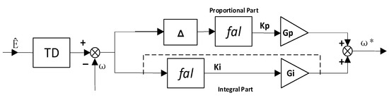
Figure 8.
Nonlinear adaptive PI controller structure.
The TD part of the controller consists of a nonlinear saturation function sin, as shown in the following equation:
where the m function is the independent variable, and are the input variables, and sgn(x) is the sign function:
An improvement of the Fal function is as follows:
In the formula, α is the tracking effect influence factor, which decreases when the filtering effect becomes worse and the tracking effect becomes better; represents the filtering effect influence factor, where the value of δ affects the range of the nonlinear interval of the Fal(e, α, δ) function; and e is the input error. The signal error is inversely proportional to the feedback gain generated by the Fal function, and the application of the Fal function gives the system good fast and stable performance.
In the steady-state operation of a nonlinear inverter, the error range remains relatively small. However, to prevent large disturbances under special conditions that could lead to increased errors and potential system instability, an improved Fal function is introduced. This modification imposes a constraint within a predefined δ-range, where δ serves as the saturation parameter, effectively enhancing system robustness and stability.
The output value ω* of the nonlinear PI module is as follows:
In the above equation,
e represents the difference between the frequency feedback value and the reference value.
Kp and Ki are the proportional and integral parameters, which are adaptively adjusted by the algorithm.
Gp and Gi are the gain coefficients of the proportional and integral components, respectively, and are optimized based on operational results. Here, they are set to 1.2 and 1, respectively.
α1 and α0 are tracking effect influence factors, constrained within the range 0 < α1 < α0 < 1. α1 and α0 are assigned values of 0.15 and 0.3, respectively.
δ0 and δ1 are filtering effect influence factors, set to 0.01 and 0.015, respectively.
The nonlinearity of the function is influenced by α, and a smaller value of α results in a higher degree of nonlinearity, while a larger value weakens the nonlinearity. The parameter δ determines the range of the nonlinear region of the Fal(e, α, δ) function. A larger value of δ increases the linear range, while a smaller value reduces it. Here, δ is set to 1.
5. Simulation Analysis
5.1. Simulation Model Building
Based on the dual-loop inverter control system block diagram shown in Figure 5, a Simulink simulation model of the dual-loop control system is constructed. The basic parameter settings for the simulation model are provided in Table 2.
Table 2.
Model parameters.
5.2. Simulation Waveforms and Analysis
Figure 9 illustrates the input–output waveforms for both the standard and improved Fal functions. By comparing Figure 9a and Figure 9b, it can be observed that in the adaptive controller using the improved Fal function, when the error exceeds one, the value of the improved Fal function is constrained within the range of zero to one. This constraint significantly reduces the function’s value compared to the standard Fal function, thus diminishing the gain associated with large errors and mitigating the impacts of such errors on system performance.

Figure 9.
Fal function input signal adaptive tracking. (a) Fal function; (b) improved Fal function.
Figure 10 presents the Bode plots of the system transfer function under two conditions: conventional PI control and adaptive frequency compensation. After compensation, the system’s loop gain amplitude–frequency characteristic curve crosses the 0 dB line at a frequency of 1500 Hz. The loop gain decreases at a rate of −20 dB/dec in the low-frequency range, and the phase margin increases to 70.6°, which is higher than that before compensation. This improvement in the phase margin enhances the system’s stability and results in better dynamic performance.

Figure 10.
Bode plot of the PI closed-loop transfer function.
Figure 11a shows the output voltage and current waveforms of the three-phase inverter. The voltage peak is 310 V and the current peak is 60 A, with a phase difference of 120° between each phase waveform. Figure 11b presents the voltage and current waveform of one phase of the three-phase inverter output. As observed from the figure, within the first 0.03 s of output, there is a slight fluctuation in the current, after which the waveform stabilizes and approximates a smooth sinusoidal form. The waveform becomes stable thereafter.
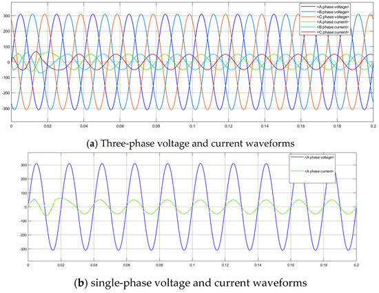
Figure 11.
Inverter output three-phase voltage and current waveforms. (a) Three-phase voltage and current waveforms; (b) single-phase voltage/current waveforms.
The waveforms of current and voltage variations during sudden load increases and decreases of the system is shown in Figure 12. When the system undergoes sudden load increases and decreases, Comparison of the output current and voltage waveform changes of the two control methods is shown in Figure 13. By comparing with conventional PI control, when the load has a sudden change at 0.1 s and recovers at 0.11 s, the system under the conventional PI control stabilizes at 0.1187 s, with an experience time of about 0.0087 s and a large overshoot. The system under adaptive compensation control stabilizes at 0.1141 s, with an experience time of about 0.0041 s and a much smaller overshoot. Adaptive PI has better regulation performance. The comparison of output waveforms is shown in Figure 13.
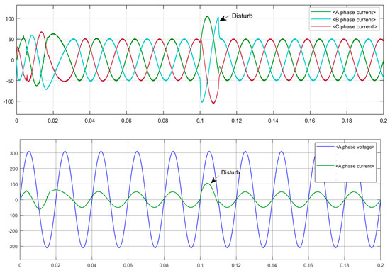
Figure 12.
Output current–voltage waveforms during a sudden load application.
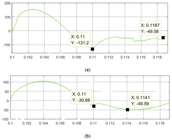
Figure 13.
Waveform of the inverter output current variation under sudden load changes for different control strategies. (a) Conventional PI control; (b) adaptive compensation PI control.
The grid voltage is transformed into the dq coordinate system of the inverter operation, and the waveforms of the d-axis and q-axis current components in the rotating dq coordinate system are shown in Figure 14. The q-axis current component is zero. When a sudden load is applied, the output d-axis current waveform stabilizes within one cycle, while the q-axis component remains zero and the waveform stays stable. The control system adjusts the q-axis component of the synthetic vector Ê, ensuring that the dq coordinate system rotates synchronously with Ê. After transformation, the d- and q-axis current components remain stable, exhibiting good dynamic performance and meeting the control requirements. This effectively ensures the stable output of active and reactive power, thus maintaining the stability of the inverter system’s power distribution.

Figure 14.
Waveforms of the dq-axis component current in a rotating coordinate system. (a) Waveform of the q-axis component, id; (b) waveform of the q-axis component, iq.
Power control is based on the reference current signal, which is used to control the set values of id∗ and iq∗. By combining the current feedback values, the system adjusts the three-phase modulation wave duty cycles through a dual closed-loop control, thereby regulating the inverter’s active and reactive power output. The output active power starts at 10 kW and transitions to 20 kW in the middle, with the reactive power remaining at 0. The simulation waveforms are shown in Figure 15. The output power effectively tracks the given reference signal.
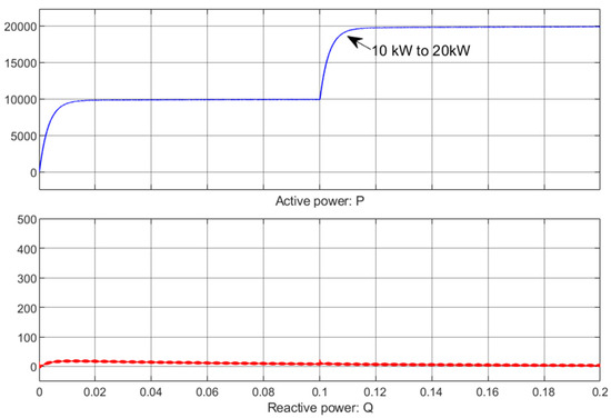
Figure 15.
Inverter output power distribution.
Since the PI controller is essentially under linear control, it is weak in suppressing higher-order harmonics and has a higher harmonic component; the PI control relies on the integral term, resulting in a slower dynamic response and larger voltage and current fluctuations under sudden load changes. From the harmonic spectrograms shown in Figure 16, the voltage/current harmonics of the improved control algorithm combined with the Fal function are lower than the PI control, more sensitive to error variations, respond faster, and have better dynamic performance. The combination of Fal function control avoids the integral saturation problem in the PI controller, improves the steady state accuracy and has better steady state performance. As shown in Figure 17, the total harmonic distortion of the voltage spectrum is 1.89 percent, with the maximum 6th harmonic not exceeding 0.8 percent. The harmonic distortion rate is small, and the output waveform is close to sinusoidal.
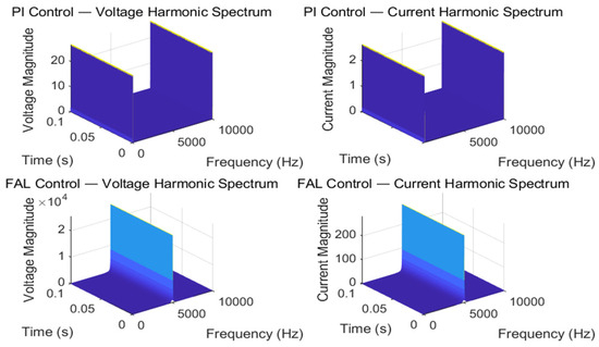
Figure 16.
Inverter output voltage/current harmonic spectra.
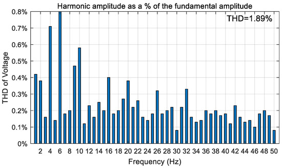
Figure 17.
Harmonic spectrum of the inverter output voltage.
6. Conclusions
The inverter control system is a nonlinear system, while traditional PI controllers are inherently linear. In a steady-state condition, the output frequency error remains within a small range of the set value. However, under special disturbances, larger perturbations can occur, which increase the error and ultimately destabilize the system. By utilizing frequency feedback, the frequency variation is controlled, which in turn governs the phase change. The improved Fal function transforms the tracking variable from error to the rate of change of the error, reducing the input value range and differentiating the frequency difference. This enhances the sensitivity of the control system to error changes and accelerates the response, enabling faster tracking. The Fal function improves the system’s dynamic response capability and exhibits strong nonlinear control characteristics, allowing for a rapid response to load disturbances and providing better system stability.
The three-phase inverter, based on adaptive frequency compensation under droop control, exhibits smooth and stable output voltage and current waveforms during steady-state operation, with lower harmonic components. It effectively controls the distribution of active and reactive power outputs. In the closed-loop control system, the reference value for the inverter’s load voltage is set to 311 V, and the actual output voltage aligns with this reference value, demonstrating high tracking accuracy in the control strategy. The adaptive dual-loop control system, improved with the Fal function, offers superior steady-state control capabilities and precision, exhibiting excellent steady-state characteristics. When the load changes, the adaptive compensation control system rapidly recovers, ensuring the system’s strong dynamic performance.
The improved Fal function, through an adaptive compensation algorithm that tracks the rate of change in frequency error, enables the system to reach the steady state more quickly compared to conventional control methods. When a sudden load change occurs, the adaptive controller ensures that the inverter output voltage can rapidly and accurately track the reference voltage set by the power loop. The dual-loop control system, based on the adaptive compensation algorithm, exhibits a faster dynamic response and enhanced resistance to disturbances. As a result, the inverter control system demonstrates superior control accuracy, along with improved steady-state and dynamic performance.
Author Contributions
Conceptualization, L.F.; methodology, L.F. and H.L.; software, H.L.; validation, L.F. and Z.F.; formal analysis, L.F.; investigation, Z.F.; data curation, L.F. and Z.F.; writing—original draft preparation, L.F.; writing—review and editing, L.F.; visualization, L.F. All authors have read and agreed to the published version of the manuscript.
Funding
This research was funded by Jiangsu Provincial Department of Science and Technology, grant number BY20230707.
Data Availability Statement
The original contributions presented in this study are included in the article. Further inquiries can be directed to the corresponding author.
Acknowledgments
I would like to express my sincere thanks to all those who helped me during the writing of this thesis. I gratefully acknowledge the help of Yang Sun and Ping Li, as they have offered me valuable suggestions. In the preparation of this thesis, they have spent much time reading through each draft and provided me with good advice. I also express my gratitude to all the reviewers and editors; l have benefited a lot from their nice suggestions and professional guidance, which helped me to complete this thesis in a better way.
Conflicts of Interest
The authors declare no conflicts of interest.
References
- Wu, X.; Panda, S.K.; Xu, J. Effect of Pulse-Width Modulation Schemes on the Performance of Three-Phase Voltage Source Converter. In Proceedings of the 33rd Annual Conference of the IEEE Industrial Electronics Society (IECON), Taipei, Taiwan, 5–8 November 2007; pp. 168–173. [Google Scholar]
- Midtsund, T.; Suul, J.A.; Undeland, T. Evaluation of current controller performance and stability for voltage source converters connected to a weak grid. In Proceedings of the 2nd International Symposium on Power Electronics for Distributed Generation Systems, Hefei, China, 16–18 June 2010; IEEE: New York, NY, USA, 2010; pp. 382–388. [Google Scholar]
- Borup, U.; Blaabjerg, F.; Enjeti, P.N. Sharing of Nonlinear Load in Parallel-Connected Three-Phase Converters. IEEE Trans. Ind. Appl. 2001, 37, 1817–1823. [Google Scholar] [CrossRef]
- Su, H.; Dong, Z.; Wang, X. Improved Droop Control Strategy for Microgrids Based on Auto Disturbance Rejection Control and LSTM. Processes 2024, 12, 2535. [Google Scholar] [CrossRef]
- Zhang, W.; Wang, Y.; Han, F.; Yang, R. Composite Sliding Mode Control of Phase Circulating Current for the Parallel Three-Phase Inverter Systems. Energies 2024, 17, 1389. [Google Scholar] [CrossRef]
- Ward, L.; Subburaj, A.; Demir, A.; Chamana, M.; Bayne, S.B. Analysis of Grid-Forming Inverter Controls for Grid-Connected and Islanded Microgrid Integration. Sustainability 2024, 16, 2148. [Google Scholar] [CrossRef]
- Xu, Z.; Chen, F.; Chen, K.; Lu, Q. Research on Adaptive Droop Control Strategy for a Solar-Storage DC Microgrid. Energies 2024, 17, 1454. [Google Scholar] [CrossRef]
- Xu, X.; Gu, Y.; Guo, J.; Song, Y. Research on Improved Droop Control Strategy of Microgrid in Island Mode. In Proceedings of the 2023 6th International Conference on Energy, Electrical and Power Engineering (CEEPE), Guangzhou, China, 14–16 April 2023; pp. 480–484. [Google Scholar] [CrossRef]
- Xu, L.; Zeng, J.; Liu, J.; Zheng, J.; Li, Y. Research on a Novel Repetitive Control Strategy for Multi-Functional Grid-Connected Inverters. J. Power Supply 2025, 10, 40. [Google Scholar]
- Xu, Q.; Fu, Y.; Miao, Y.; Zhao, Y.; Luo, L. Modulation and Control Strategy of Novel Sigle-phase Grid-connected Current Source Inverter. Acta Energiae Solaris Sin. 2025, 46, 412–420. [Google Scholar] [CrossRef]
- Chen, L.; Chen, M.; Li, B.; Sun, X.; Jiang, F. Harmonic Current Suppression of Dual Three-Phase Permanent Magnet Synchronous Motor with Improved Proportional-Integral Resonant Controller. Energies 2025, 18, 1340. [Google Scholar] [CrossRef]
- Zhang, Y.; Zhao, Z. A New Fractional-order Internal Model PID Control Method for DC Speed Regulation System. Fire Control Command Control 2025, 50, 56–61 + 70. [Google Scholar]
- Zhang, D.; Li, W. Research on Six-Degree-of-Freedom Series Manipulator Based Fractional Order Sliding Mode Active Disturbance Rejection Control. Journal of Dynamics and Control 2025, 23, 49–58. [Google Scholar] [CrossRef]
- Tu, B.; Xu, X.; Gu, Y.; Deng, K.; Xu, Y.; Zhang, T.; Gao, X.; Wang, K.; Wei, Q. Improved Droop Control Strategy for Islanded Microgrids Based on the Adaptive Weight Particle Swarm Optimization Algorithm. Electronics 2025, 14, 893. [Google Scholar] [CrossRef]
- Rong, H.; Chen, Y. Improved Droop Control Strategy of Microgrid Based on Optimized Particle Swarm Algorithm. In Proceedings of the 2020 Chinese Automation Congress (CAC), Shanghai, China, 6–8 November 2020; pp. 2324–2329. [Google Scholar] [CrossRef]
- Zhang, L.; Zheng, H.; Hu, Q.; Su, B.; Lyu, L. An Adaptive Droop Control Strategy for Islanded Microgrid Based on Improved Particle Swarm Optimization. IEEE Access 2020, 8, 3579–3593. [Google Scholar] [CrossRef]
- Huang, X.; Chen, C. Improved Droop Control Scheme for Reactive Power Sharing of Parallel Inverter System. In Proceedings of the 2020 IEEE 1st China International Youth Conference on Electrical Engineering (CIYCEE), Wuhan, China, 8–10 November 2020; pp. 1–6. [Google Scholar] [CrossRef]
- Kaewnukultorn, T.; Hegedus, S. Impact of Impedances and Solar Inverter Grid Controls in Electric Distribution Line with Grid Voltage and Frequency Instability. Energies 2024, 17, 5503. [Google Scholar] [CrossRef]
- Vekić, M.; Rapaić, M.; Todorović, I.; Grabić, S. Decentralized Goal-Function-Based Microgrid Primary Control with Voltage Harmonics Compensation. Energies 2024, 17, 4961. [Google Scholar] [CrossRef]
- Qiu, L.; Gu, M.; Chen, Z.; Du, Z.; Zhang, L.; Li, W.; Huang, J.; Fang, J. Oscillation Suppression of Grid-Following Converters by Grid-Forming Converters with Adaptive Droop Control. Energies 2024, 17, 5230. [Google Scholar] [CrossRef]
- Zhou, Z.; Zou, H. Improved Droop Control Strategy Based on Consensus Algorithm. In Proceedings of the 2023 3rd International Conference on Electrical Engineering and Control Science (IC2ECS), Hangzhou, China, 20–22 October 2023; pp. 1696–1700. [Google Scholar] [CrossRef]
- Khooban, M.H.; Gheisarnejad, M. A Novel Deep Reinforcement Learning Controller Based Type-II Fuzzy System: Frequency Regulation in Microgrids. IEEE Trans. Emerg. Top. Comput. Intell. 2021, 5, 689–699. [Google Scholar] [CrossRef]
- Zeng, H.; Zhao, E.; Zhou, S.; Han, Y.; Yang, P.; Wang, C. Adaptive droop control of a DC microgrid based on current consistency. Power Syst. Prot. Control 2022, 50, 11–21. [Google Scholar]
- Kim, D.-Y.; Lee, J.-H. Compensation of Interpolation Error for Look-Up Table-Based PMSM Control Method in Maximum Power Control. Energies 2021, 14, 5526. [Google Scholar] [CrossRef]
- Ding, M.; Tao, Z.; Hu, B.; Tan, S.; Yokoyama, R. Parallel Operation Strategy of Inverters Based on an Improved Adaptive Droop Control and Equivalent Input Disturbance Approach. Electronics 2024, 13, 486. [Google Scholar] [CrossRef]
- Ma, J.; Wang, X.; Liu, J.; Gao, H. An Improved Droop Control Method for Voltage-Source Inverter Parallel Systems Considering Line Impedance Differences. Energies 2019, 12, 1158. [Google Scholar] [CrossRef]
- Ren, B.; Sun, X.; Chen, S.; Liu, H. A Compensation Control Scheme of Voltage Unbalance Using a Combined Three-Phase Inverter in an Islanded Microgrid. Energies 2018, 11, 2486. [Google Scholar] [CrossRef]
Disclaimer/Publisher’s Note: The statements, opinions and data contained in all publications are solely those of the individual author(s) and contributor(s) and not of MDPI and/or the editor(s). MDPI and/or the editor(s) disclaim responsibility for any injury to people or property resulting from any ideas, methods, instructions or products referred to in the content. |
© 2025 by the authors. Licensee MDPI, Basel, Switzerland. This article is an open access article distributed under the terms and conditions of the Creative Commons Attribution (CC BY) license (https://creativecommons.org/licenses/by/4.0/).