4.1. Basic Principles of the Fibonacci Search Method
An integer sequence {F
k}(k = 0, 1, …) satisfying the following conditions is called a Fibonacci sequence:
Assume f(x) has only one minimum point in the closed interval [a
0, b
0]. The Fibonacci search method for finding the optimal value of a single-variable unimodal function involves the following steps: first, select two test points x
1 and x
2 and within the initial interval [a
0,b
0], calculate f(x
1) and f(x
2), compare their values, narrow the search range, and repeat the process iteratively until the search interval is smaller than a predefined threshold [
14].
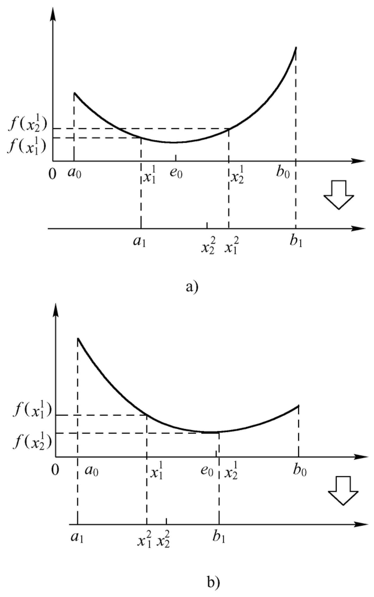
During the first iteration, the test points
and
are selected within the interval [a
0, b
0] as follows:
where the definition of parameter n is the number of iterations, the length of the interval
equals that of
, and
. By comparing f(x
1) and f(x
2), the search interval is reduced iteratively until the relative precision is met [
15].
If
, then eliminate the interval
and select the second trial points
and
within the remaining interval
, as shown in
Figure 4. At this point
,
, and
, and the formula for selecting the second trial point is
From the equation above
, and if
, the interval
is eliminated. The remaining interval
is then searched by selecting new trial points
and
(see
Figure 4b), where
,
, and
(or an equivalent update rule) [
16]. The same principle applies in further steps,
.
After multiple iterations following the aforementioned rules, the search range gradually converges toward the optimal value of the function. At this point, the optimal value needs to be determined based on the relative precision δ of the interval reduction [
17]. A relative precision threshold δ is defined, and its selection principle is as follows: Assuming the final search interval is [a
n−1, b
n−1], the condition (b
n−1 − a
n−1) ≤ δ(b
0 − a
0) must be satisfied. Once the required relative precision δ is achieved, the search can terminate. A smaller δ improves the accuracy of the optimal value but slows down convergence. By iteratively computing function values, the search interval can be narrowed down to meet the desired relative precision. When the number of function evaluations reaches F
n ≥ 1/δ, the optimal value of the function f(x) is obtained [
18].
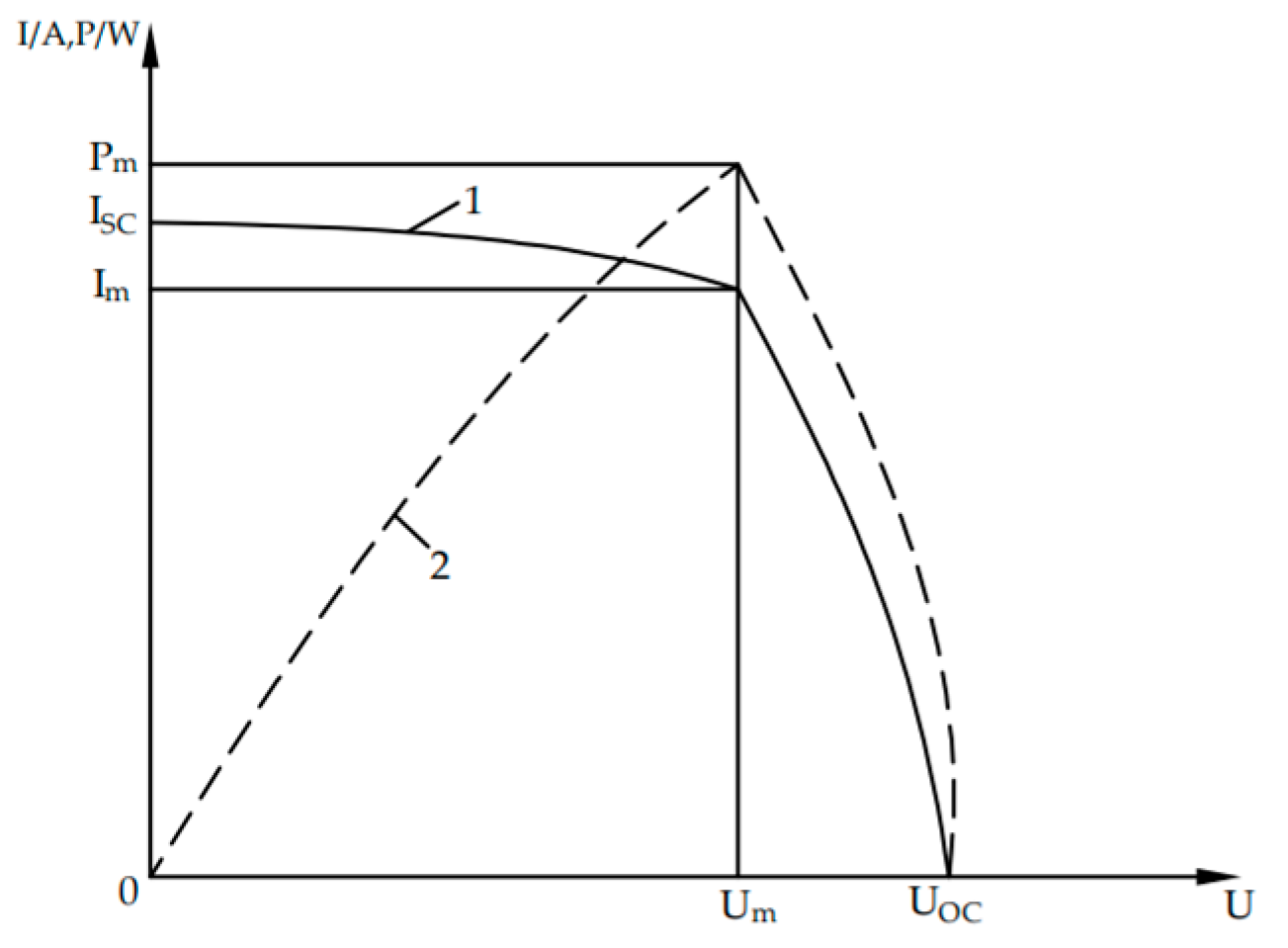
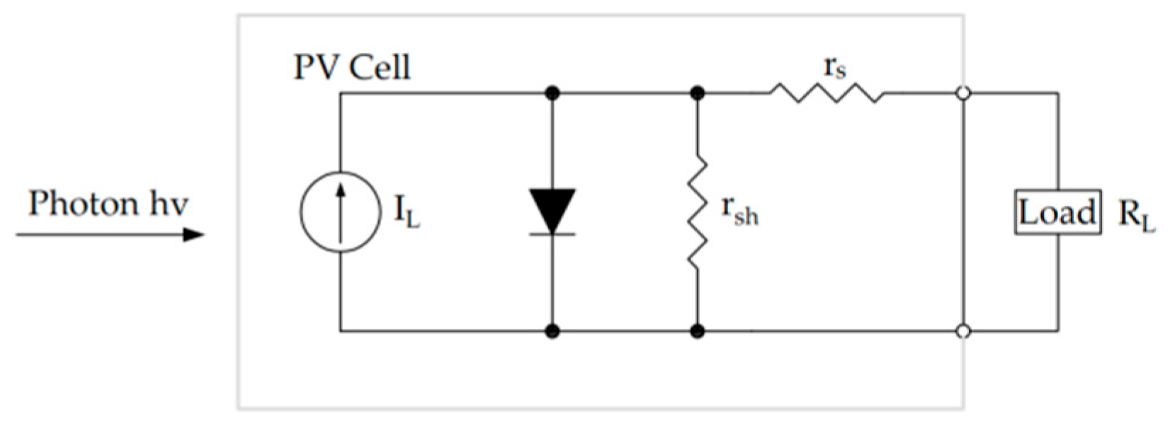
When the Fibonacci search algorithm is applied for maximum power point tracking (MPPT) in photovoltaic (PV) arrays, the output voltage of the PV array can be represented as the independent variable x, while the output power is expressed as f(x). By leveraging the P-U characteristic curve of the PV array, the maximum output power can be tracked and achieved in real time by adjusting the output voltage. In the traditional Fibonacci search method, the relative precision δ determines the optimal value by constraining the range of the independent variable. However, from the perspective of the optimal value itself, it is not precisely quantified [
19]. The ultimate goal of MPPT is to locate the maximum output power of the PV array. If the traditional Fibonacci search method is used for PV array MPPT, a significant issue arises near the maximum power point: the output voltage exhibits a high sensitivity to power variations. As a result, the tracked maximum power may deviate from the true value, leading to inaccuracies.
To address the aforementioned issues, the concept of absolute precision ε can be introduced, and the iteration termination condition can be modified as follows: Iteration stops when both conditions (b
n−1 − a
n−1) ≤ δ(b
0 − a
0) and
are satisfied, thereby obtaining the maximum power point (MPP) voltage and the maximum output power of the array. By adding the supplementary condition
, the function f(x) is constrained in its value range. This enhancement not only increases the output power of the PV array but also makes the improved search method more precise than traditional approaches, effectively reducing errors [
20].
Meanwhile, the use of high-precision measurement systems further ensures the accuracy of the results. The accuracy and sampling rate of different sensors are shown in
Table 2.
When using the traditional Fibonacci search algorithm for MPPT in photovoltaic power generation systems, there is a problem of computational complexity. The quantitative analysis of the computational complexity comparison of the improved Fibonacci search algorithm in photovoltaic MPPT is as follows:
(1) The complexity of the traditional Fibonacci algorithm.
① Time complexity: , where δ is the relative accuracy.
② Under typical parameters, the following applies:
Each iteration requires two power calculations (f(x1), f(x2));
The number of iterations required for convergence is .
For example, when the initial interval is [0, 50 V] and δ = 0.01 V, approximately 24 iterations are required.
(2) Improved algorithm optimization.
① Dynamic accuracy adjustment: δ k = max (0.02, 0.1e − αt).
② The complexity is reduced to .
③ The number of iterations decreased by 38% (measured from 24 to 15 times).
The performance quantification comparison of different indicators is shown in
Table 3.
4.2. MPPT Control Flow
It is assumed that the structure of the PV Array is m × n, there are m groups of series-connected PV arrays with n PV arrays in each group, and the open circuit voltage of the arrays under normal light conditions is UOC_N. UMPP_N is the voltage at the point of maximum power, PMPP_N is the maximum output power, and cN is the scaling factor.
(1) The physical meaning and determination method of the proportionality coefficient cN.
cN is a key parameter used to divide the voltage search interval, defined as cN = VMPP, N/VOC, N.
Among them, VMPP, N is the maximum power point voltage under standard conditions, while VOC, N is the open circuit voltage. Its physical meaning is to reflect the inherent proportional relationship between the maximum power point voltage and the open circuit voltage of the photovoltaic array.
(2) The impact of cN on algorithm performance.
① Efficiency impact analysis.
The impact of cN deviation on Fibonacci search and quantization results is shown in
Table 4.
② Dynamic performance relationship
Convergence speed: The closer cN is to the true proportion, the more accurate the search interval, and the fewer convergence iterations.
Anti interference: When the cN error is greater than 15%, the algorithm may fall into local extremum under shadow conditions.
Conclusion:
(1) The accuracy of cN directly affects the efficiency of the algorithm, and the error needs to be controlled within ±5%;
(2) Adopting a dynamic update strategy can increase system revenue by 3–5%;
(3) In scenes with large temperature fluctuations or frequent shadows, it is necessary to achieve adaptive adjustment of cN.
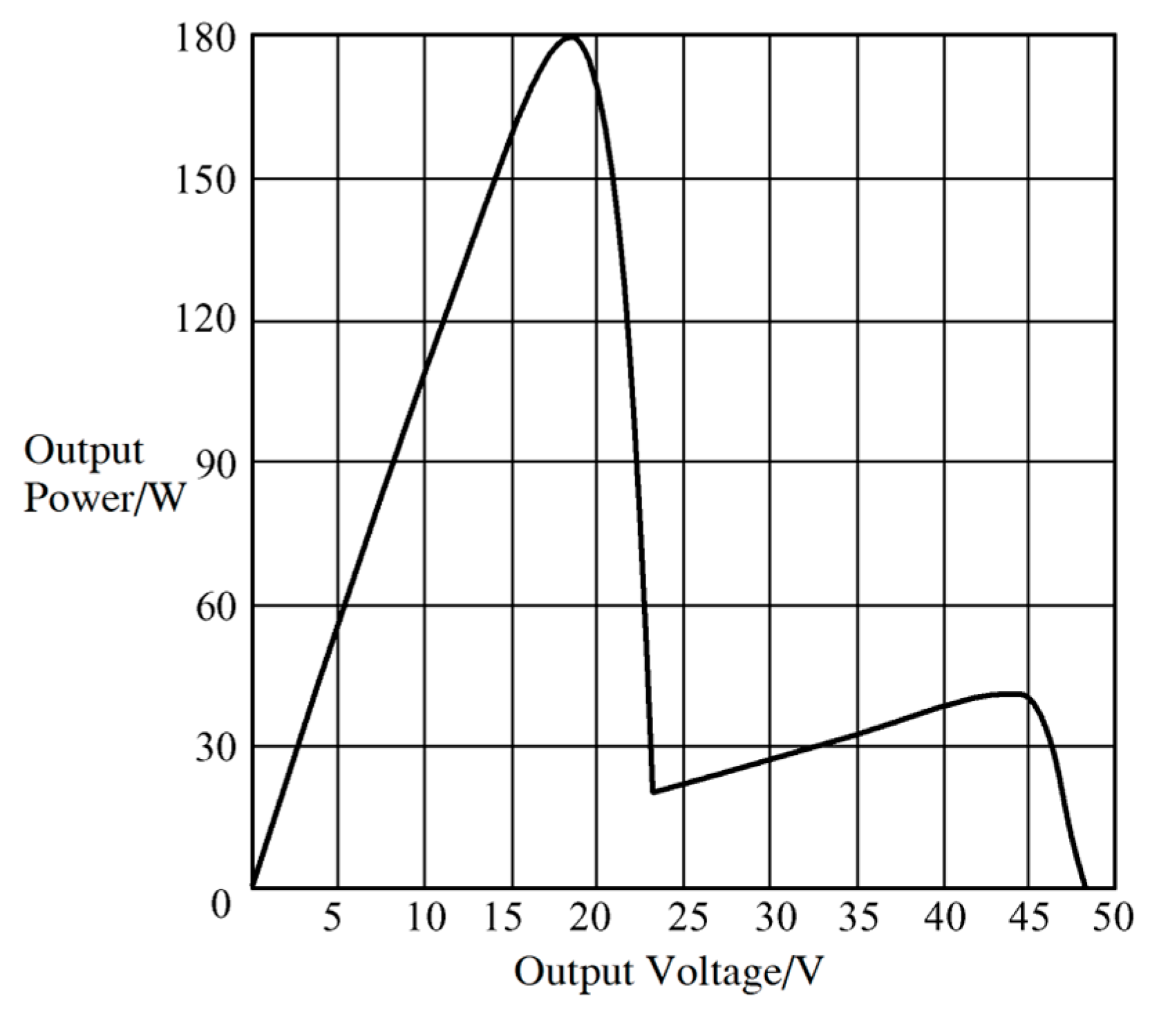
According to the aforementioned analysis of the PV array output characteristics, it can be known that in the voltage interval [a
i, b
i], where a
i = [(i + 1)c
N − 1]U
OC_N, b
i = [(i − 1)c
N + 1]U
OC_N, i = 1, 2, …, n, the PV array may have a peak power point whose P-U output in the aforementioned (n − 1) voltage intervals exhibits single-peak characteristics. In the voltage interval [c,d], where c = [(n − 2)c
N + 1]U
OC_N,d = [(n + 2)c
N − 1]U
OC_N, the peak power point may exist in the PV array, and its P-U output no longer has a single-peak characteristic [
21].
In the voltage interval [a
i, b
i], the local peak power of the PV array is tracked with the improved Fibonacci search method, and in the voltage interval [c, d], the local peak power of the PV array is tracked with the improved variable-step-size perturbation observation method, and the global maximum power point of the PV array is obtained by comparing the peak power points [
22]. The control flow of the global maximum power point tracking algorithm is shown in
Figure 5.
In the case of uniform illumination, in order to select the appropriate control algorithm, the PV array needs to judge the light environment before the maximum power tracking. The method of judging the light environment involves setting the operating voltage to kU
MPP_N, with the output power of the PV array, P
MPP_k, then calculated one by one, where k = 1, 2, …, n, when n is a positive integer; if P
MPP_1 < P
MPP_2 < … < P
MPP_n and P
MPP_n > 0.9 mnP
MPP_N, then it means that the PV array is in a uniform light environment, in which case, set a
0 = [(i + 1)c
N − 1]U
OC_N, b
0 = [(i − 1)c
N + 1]U
OC_N and track the maximum power of the PV array using the Fibonacci search method [
23]. As long as one of the above two conditions is not satisfied, it is determined that the PV array is in a complex light environment. In this case, set a
0 = [(i + 1)c
N − 1]U
OC_N,b
0 = [(i − 1)c
N + 1]U
OC_N and track the local maximum power of the PV array, P
i, in the interval by using the Fibonacci search method, and if Pi exceeds P
MAX, then set P
MAX = P
i, increasing i by 1 and continuing the power tracking by checking the next voltage interval until i reaches n − 1. When i = n, the PV array is observed with variable step-size perturbations in the voltage range [U
begin, U
end], so that its maximum power P
n is tracked. If P
n exceeds P
MAX, then U
begin = [(n − 2)c
N + 1]U
OC_N, U
end = [(n + 2)c
N − 1]U
OC_N, the maximum power of the PV array over the entire voltage range is P
MAX, and the corresponding voltage at the point of maximum power is U
MAX = U
n. Now, the PV array voltage is adjusted to the operating point U
ref = U
MAX, and this is carried out to ensure that the maximum power point tracking of the PV array always outputs maximum power [
24].


