Abstract
At present, photovoltaic power generation is becoming increasingly popular, and one of its major drawbacks is the low photoelectric conversion efficiency of photovoltaic cells. In order to improve power generation efficiency, an equivalent circuit model of photovoltaic cells and a simulation structure of photovoltaic power generation systems have been established. The working principle and MPPT (Maximum Power Point Tracking) control process of the improved Fibonacci linear search algorithm have been analyzed to achieve the goal of improving power generation efficiency. The improved Fibonacci linear search algorithm is applied in the MPPT technology of photovoltaic power generation system, and simulation experiments are conducted. Through analysis and simulation, MPPT can quickly track the maximum power point when the external lighting conditions change and has good tracking effect.
1. Introduction
One of the main disadvantages of PV (photovoltaic) power generation systems is the low photoelectric conversion efficiency of PV cells. Typically, the conversion efficiency of polycrystalline silicon cells ranges from 12% to 14%, while that of monocrystalline silicon cells ranges from 14% to 18%. Considering inverter efficiency, the overall efficiency of PV systems is only slightly above 10% [1]. To improve solar energy utilization, methods include enhancing the conversion efficiency of PV arrays or modifying the structure and control strategies of inverters to ensure the PV array operates near the maximum power point, known as Maximum Power Point Tracking (MPPT).
PV arrays are power-unstable devices with complex nonlinear output characteristics, influenced by external environmental conditions such as solar irradiance, temperature, and load. Therefore, ensuring the PV array operates at the maximum power point is crucial for improving photoelectric conversion efficiency [2]. This paper provides a detailed introduction to the basic principles and main algorithms of MPPT in PV power generation systems.
The traditional MPPT methods for photovoltaic power generation systems mainly include the constant voltage tracking method, conductance increment method, and interference observation method (also known as the hill climbing method). These methods have certain effects under different lighting intensities and temperature conditions, but there are also some limitations [3].
For example, the limitations of the constant voltage tracking method are prominent. In total, 76% of the open circuit voltage is selected as the fixed voltage, and the photovoltaic panel is operated at this voltage to approximate the maximum power tracking. When the temperature is the same under different light intensities, the maximum power point of the solar panel almost falls on both sides of the same vertical line, which may make it difficult to accurately track the maximum power line at specific temperature moments.
The advantage of the incremental conductance method is that the direction of the reference voltage change at the next moment depends entirely on the instantaneous impedance and the magnitude of the impedance change at that moment and is independent of the operating point voltage and power at the previous moment, so there will be no misjudgment in the disturbance observation method. Therefore, it can adapt to rapid changes in light intensity, with small voltage fluctuations and high control accuracy. The disadvantage is that it is susceptible to interference from clutter signals and can cause significant misoperation [4]. In practical operation, usually very small values of dI and dU are taken, which requires high precision in the collection of parameters such as the output voltage and output current of photovoltaic devices. The accuracy of sensors is also required to be high, and the calculation process is relatively complex. It must be adjusted gradually to approach the maximum power point and cannot be quickly adjusted to the maximum power point.
Although the perturbation observation method has the advantages of simple logic and easy implementation, it may make errors in the case of changes in light intensity. When the illumination rapidly decreases, the output power of the photovoltaic module will also change due to the characteristics presented by the P-V curve of the photovoltaic module, which may affect the judgment of the disturbance direction [5].The comparison of the performance of various MPPT algorithms is shown in Table 1.

Table 1.
Performance comparison of MPPT algorithm for photovoltaic power generation system.
Overall, various MPPT methods have their advantages and disadvantages, and the choice of method depends on specific application scenarios and environmental conditions. This article introduces an improved Fibonacci search algorithm that can accurately and quickly track the maximum power of photovoltaic arrays under different tracking strategies for uniform lighting and shadow conditions and is applicable to photovoltaic arrays of any topology.
2. Principle of Maximum Power Point Tracking Control Technology for Photovoltaic Power Generation System
In photovoltaic power generation systems, the voltage values at both ends of photovoltaic cells are not fixed when outputting maximum power under different light intensities. Moreover, when the operating temperature changes, the voltage values will also change for the same maximum power under the same light intensity. The output of a photovoltaic cell is closely related to the intensity of light and the temperature of the environment. In order to ensure that the photovoltaic cell can have maximum power output at any light intensity and temperature, that is, the photovoltaic cell always operates at the maximum power point, the first step is to determine the position of the maximum power point on the photovoltaic cell’s volt ampere characteristic curve [6].
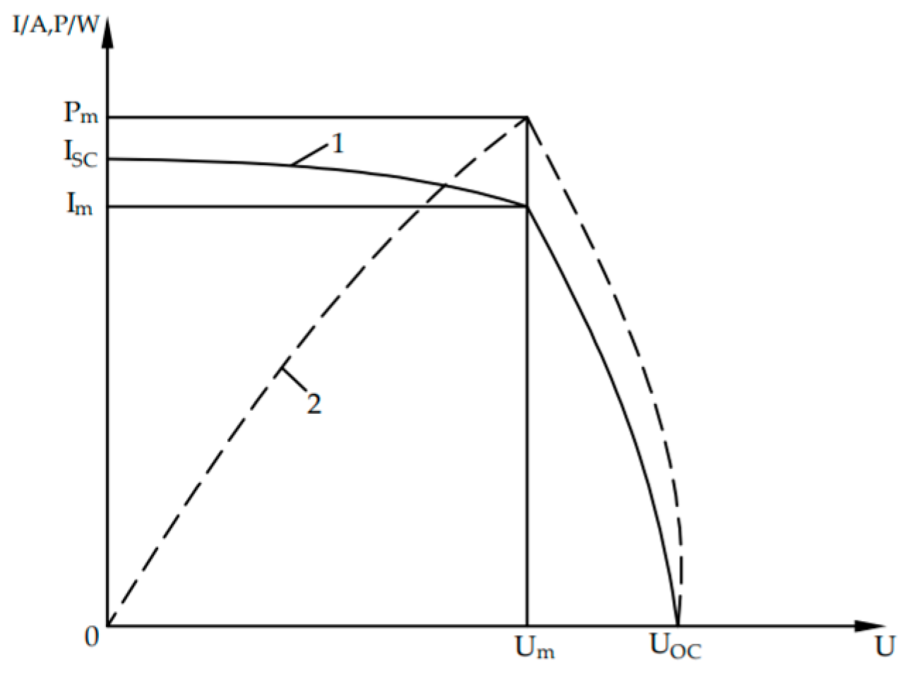
Figure 1 shows the current (power)–voltage relationship curve of a photovoltaic cell, which represents the relationship between the output current I (power P) and voltage U of the cell under specific light intensity and temperature. From the previous analysis of the output characteristics of photovoltaic cells, it can be seen that both curve 1 and curve 2 indicate the characteristics of the cells and have obvious nonlinear features. Curve 2 is similar to a parabola; that is, when the photovoltaic cell outputs the maximum power Pm (ImUm), the maximum power point voltage (maximum operating voltage) Um is less than the open circuit voltage UOC, and the current (maximum operating current) Im at the maximum power point is less than the short-circuit current ISC. When the battery voltage varies between 0 and Um, the power curve is an increasing function, and when the battery voltage is between Um and UOC, the power curve is a decreasing function. The output power of photovoltaic cells mainly depends on the intensity of light and their operating temperature. According to the I-U and P-U characteristic curves of photovoltaic cells at different temperatures, as the operating temperature increases, the short-circuit current ISC slightly increases, the open circuit voltage UOC and the maximum power point voltage Um decrease, and the maximum output power Pm of the photovoltaic cell decreases. According to the I-U and P-U characteristic curves under different light intensities, it can be concluded that the ISC value of the same battery is directly proportional to the light intensity; the maximum output power Pm also increases with the increase in light intensity [7].
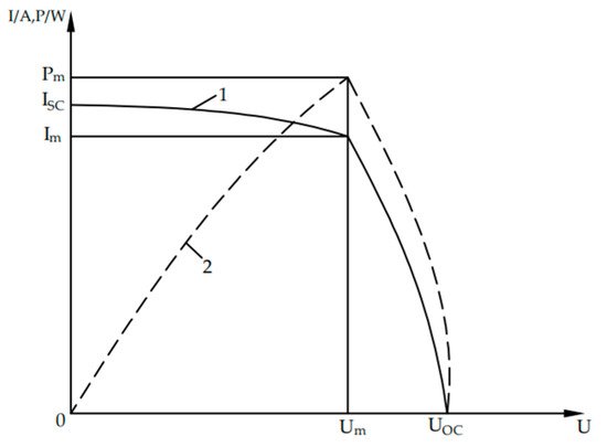
Figure 1.
Photovoltaic cell current (power)–voltage relationship curve.
In order to achieve the maximum energy output of photovoltaic arrays under current illumination under any external conditions, the maximum power point tracking problem of photovoltaic arrays is proposed [8]. With the increasing popularity of photovoltaic power generation systems, the high cost and low conversion efficiency of photovoltaic power generation systems make the research on maximum power point tracking technology increasingly important. The maximum power point tracking (MPPT) control strategy is to detect the output power of the photovoltaic array in real time, use a certain control algorithm to predict the possible maximum power output of the photovoltaic array under the current working conditions, and meet the requirements of maximum power output by changing the current impedance situation. In this way, even if the junction temperature of the photovoltaic cell increases and the output power of the array decreases, the system can still operate at its optimal state under the current operating conditions [9]. Due to the nonlinear output characteristics of photovoltaic cells, mathematical analysis is not easy. Simple linear circuits can be used to study the basic principles of maximum power point tracking.
According to the impedance matching principle in circuit theory, in a linear circuit, when the equivalent resistance of the external load is equal to the internal resistance of the power supply, the external load can obtain the maximum output power. That is to say, when the load resistance is equal to the internal resistance of the power supply, the power supply has the maximum power output. Although photovoltaic cells and power electronic converters are both nonlinear, they can be considered linear circuits in the short term [10]. The photovoltaic cell is modeled as a DC power source and the power electronic converter as an external resistive load, the equivalent resistance of the power electronic converter is adjusted to always follow the internal resistance changes in the photovoltaic cell in different external environments, and the two loads are dynamically matched to obtain the maximum output power on the output side of the power electronic converter, achieving MPPT of the photovoltaic cell [11].
3. Modeling of Photovoltaic Power Generation System
3.1. Equivalent Circuit Model of PV Cells
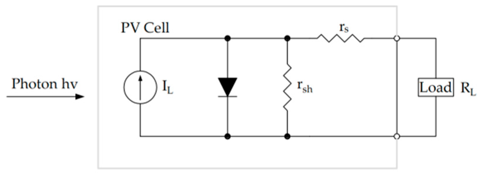
The PV cell can be described using the equivalent circuit model shown in Figure 2. When connected to a load R, the generated photocurrent IL flows through the load, producing terminal voltage U [12].
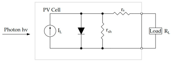
Figure 2.
Equivalent circuit model of a PV cell.
From the equivalent circuit model in Figure 1, the output characteristic equation is as follows:
where i is the output current of the PV cell; rs is the internal equivalent series resistance; IL is the photocurrent source current; n is the diode ideality factor; Io is the reverse saturation current of the diode; k is the Boltzmann constant; q is the electron charge; T is the operating temperature of the PV cell; U is the output voltage of the PV cell; and rgh is the internal equivalent parallel impedance.
3.2. Simulation Structure of PV Power Generation System
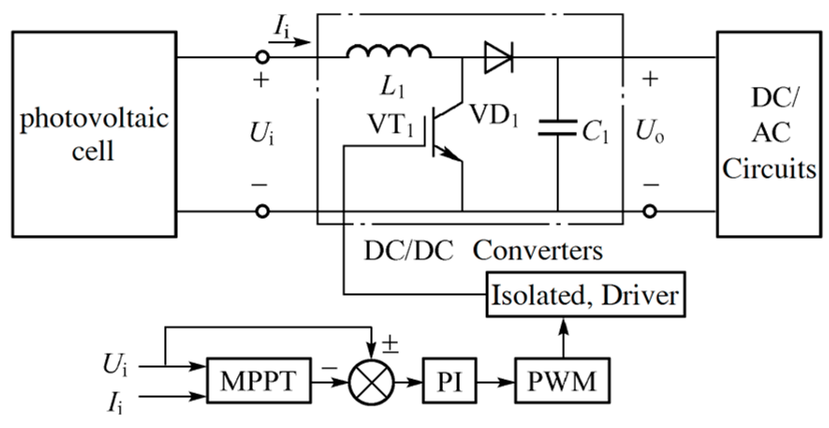
The MPPT structure of the PV power generation system consists of PV cells, a boost converter, an MPPT controller, and a PWM (Pulse Width Modulation) drive circuit, as shown in Figure 3. The MPPT controller adjusts the switching state of the IGBT (insulated gate bipolar transistor) in the Boost circuit by receiving the output current I and voltage U of the PV cell to generate PWM drive pulses [13].
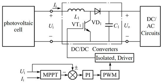
Figure 3.
System block diagram.
4. Improved Fibonacci Linear Search Algorithm
4.1. Basic Principles of the Fibonacci Search Method
An integer sequence {Fk}(k = 0, 1, …) satisfying the following conditions is called a Fibonacci sequence:
Assume f(x) has only one minimum point in the closed interval [a0, b0]. The Fibonacci search method for finding the optimal value of a single-variable unimodal function involves the following steps: first, select two test points x1 and x2 and within the initial interval [a0,b0], calculate f(x1) and f(x2), compare their values, narrow the search range, and repeat the process iteratively until the search interval is smaller than a predefined threshold [14].
During the first iteration, the test points and are selected within the interval [a0, b0] as follows:
where the definition of parameter n is the number of iterations, the length of the interval equals that of , and . By comparing f(x1) and f(x2), the search interval is reduced iteratively until the relative precision is met [15].
If , then eliminate the interval and select the second trial points and within the remaining interval , as shown in Figure 4. At this point , , and , and the formula for selecting the second trial point is
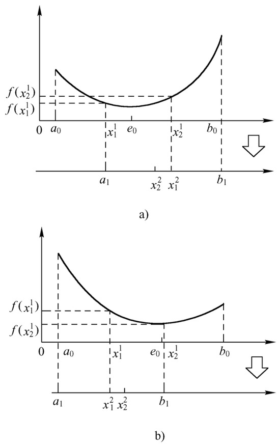
Figure 4.
Illustration of the Fibonacci search rule. (a) is a schematic diagram of , and (b) is a schematic diagram of .
From the equation above , and if , the interval is eliminated. The remaining interval is then searched by selecting new trial points and (see Figure 4b), where , , and (or an equivalent update rule) [16]. The same principle applies in further steps, .
After multiple iterations following the aforementioned rules, the search range gradually converges toward the optimal value of the function. At this point, the optimal value needs to be determined based on the relative precision δ of the interval reduction [17]. A relative precision threshold δ is defined, and its selection principle is as follows: Assuming the final search interval is [an−1, bn−1], the condition (bn−1 − an−1) ≤ δ(b0 − a0) must be satisfied. Once the required relative precision δ is achieved, the search can terminate. A smaller δ improves the accuracy of the optimal value but slows down convergence. By iteratively computing function values, the search interval can be narrowed down to meet the desired relative precision. When the number of function evaluations reaches Fn ≥ 1/δ, the optimal value of the function f(x) is obtained [18].
When the Fibonacci search algorithm is applied for maximum power point tracking (MPPT) in photovoltaic (PV) arrays, the output voltage of the PV array can be represented as the independent variable x, while the output power is expressed as f(x). By leveraging the P-U characteristic curve of the PV array, the maximum output power can be tracked and achieved in real time by adjusting the output voltage. In the traditional Fibonacci search method, the relative precision δ determines the optimal value by constraining the range of the independent variable. However, from the perspective of the optimal value itself, it is not precisely quantified [19]. The ultimate goal of MPPT is to locate the maximum output power of the PV array. If the traditional Fibonacci search method is used for PV array MPPT, a significant issue arises near the maximum power point: the output voltage exhibits a high sensitivity to power variations. As a result, the tracked maximum power may deviate from the true value, leading to inaccuracies.
To address the aforementioned issues, the concept of absolute precision ε can be introduced, and the iteration termination condition can be modified as follows: Iteration stops when both conditions (bn−1 − an−1) ≤ δ(b0 − a0) and are satisfied, thereby obtaining the maximum power point (MPP) voltage and the maximum output power of the array. By adding the supplementary condition , the function f(x) is constrained in its value range. This enhancement not only increases the output power of the PV array but also makes the improved search method more precise than traditional approaches, effectively reducing errors [20].
Meanwhile, the use of high-precision measurement systems further ensures the accuracy of the results. The accuracy and sampling rate of different sensors are shown in Table 2.
Table 2.
Key sensors.
When using the traditional Fibonacci search algorithm for MPPT in photovoltaic power generation systems, there is a problem of computational complexity. The quantitative analysis of the computational complexity comparison of the improved Fibonacci search algorithm in photovoltaic MPPT is as follows:
(1) The complexity of the traditional Fibonacci algorithm.
① Time complexity: , where δ is the relative accuracy.
② Under typical parameters, the following applies:
Each iteration requires two power calculations (f(x1), f(x2));
The number of iterations required for convergence is .
For example, when the initial interval is [0, 50 V] and δ = 0.01 V, approximately 24 iterations are required.
(2) Improved algorithm optimization.
① Dynamic accuracy adjustment: δ k = max (0.02, 0.1e − αt).
② The complexity is reduced to .
③ The number of iterations decreased by 38% (measured from 24 to 15 times).
The performance quantification comparison of different indicators is shown in Table 3.
Table 3.
Performance quantitative comparison.
4.2. MPPT Control Flow
It is assumed that the structure of the PV Array is m × n, there are m groups of series-connected PV arrays with n PV arrays in each group, and the open circuit voltage of the arrays under normal light conditions is UOC_N. UMPP_N is the voltage at the point of maximum power, PMPP_N is the maximum output power, and cN is the scaling factor.
(1) The physical meaning and determination method of the proportionality coefficient cN.
cN is a key parameter used to divide the voltage search interval, defined as cN = VMPP, N/VOC, N.
Among them, VMPP, N is the maximum power point voltage under standard conditions, while VOC, N is the open circuit voltage. Its physical meaning is to reflect the inherent proportional relationship between the maximum power point voltage and the open circuit voltage of the photovoltaic array.
(2) The impact of cN on algorithm performance.
① Efficiency impact analysis.
The impact of cN deviation on Fibonacci search and quantization results is shown in Table 4.
Table 4.
Efficiency impact analysis table.
② Dynamic performance relationship
Convergence speed: The closer cN is to the true proportion, the more accurate the search interval, and the fewer convergence iterations.
Anti interference: When the cN error is greater than 15%, the algorithm may fall into local extremum under shadow conditions.
Conclusion:
(1) The accuracy of cN directly affects the efficiency of the algorithm, and the error needs to be controlled within ±5%;
(2) Adopting a dynamic update strategy can increase system revenue by 3–5%;
(3) In scenes with large temperature fluctuations or frequent shadows, it is necessary to achieve adaptive adjustment of cN.
According to the aforementioned analysis of the PV array output characteristics, it can be known that in the voltage interval [ai, bi], where ai = [(i + 1)cN − 1]UOC_N, bi = [(i − 1)cN + 1]UOC_N, i = 1, 2, …, n, the PV array may have a peak power point whose P-U output in the aforementioned (n − 1) voltage intervals exhibits single-peak characteristics. In the voltage interval [c,d], where c = [(n − 2)cN + 1]UOC_N,d = [(n + 2)cN − 1]UOC_N, the peak power point may exist in the PV array, and its P-U output no longer has a single-peak characteristic [21].
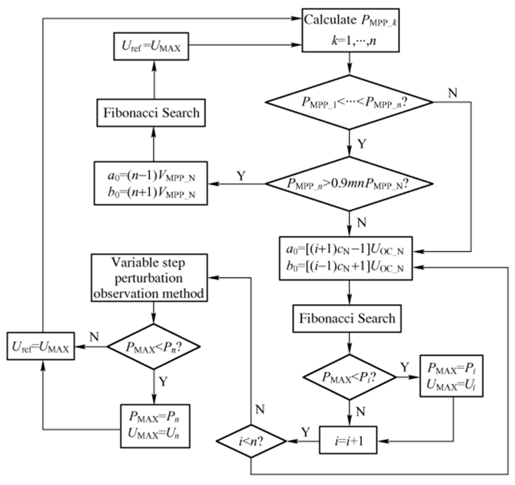
In the voltage interval [ai, bi], the local peak power of the PV array is tracked with the improved Fibonacci search method, and in the voltage interval [c, d], the local peak power of the PV array is tracked with the improved variable-step-size perturbation observation method, and the global maximum power point of the PV array is obtained by comparing the peak power points [22]. The control flow of the global maximum power point tracking algorithm is shown in Figure 5.
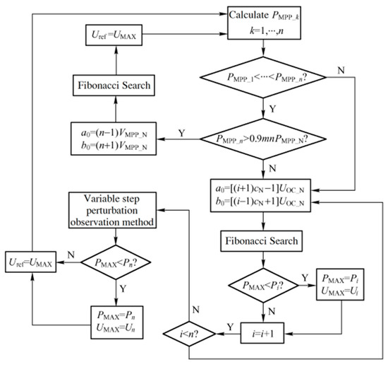
Figure 5.
Global maximum power point tracking algorithm control flow.
In the case of uniform illumination, in order to select the appropriate control algorithm, the PV array needs to judge the light environment before the maximum power tracking. The method of judging the light environment involves setting the operating voltage to kUMPP_N, with the output power of the PV array, PMPP_k, then calculated one by one, where k = 1, 2, …, n, when n is a positive integer; if PMPP_1 < PMPP_2 < … < PMPP_n and PMPP_n > 0.9 mnPMPP_N, then it means that the PV array is in a uniform light environment, in which case, set a0 = [(i + 1)cN − 1]UOC_N, b0 = [(i − 1)cN + 1]UOC_N and track the maximum power of the PV array using the Fibonacci search method [23]. As long as one of the above two conditions is not satisfied, it is determined that the PV array is in a complex light environment. In this case, set a0 = [(i + 1)cN − 1]UOC_N,b0 = [(i − 1)cN + 1]UOC_N and track the local maximum power of the PV array, Pi, in the interval by using the Fibonacci search method, and if Pi exceeds PMAX, then set PMAX = Pi, increasing i by 1 and continuing the power tracking by checking the next voltage interval until i reaches n − 1. When i = n, the PV array is observed with variable step-size perturbations in the voltage range [Ubegin, Uend], so that its maximum power Pn is tracked. If Pn exceeds PMAX, then Ubegin = [(n − 2)cN + 1]UOC_N, Uend = [(n + 2)cN − 1]UOC_N, the maximum power of the PV array over the entire voltage range is PMAX, and the corresponding voltage at the point of maximum power is UMAX = Un. Now, the PV array voltage is adjusted to the operating point Uref = UMAX, and this is carried out to ensure that the maximum power point tracking of the PV array always outputs maximum power [24].
5. Simulation Analysis of MPPT Under Localized Shadowing Conditions
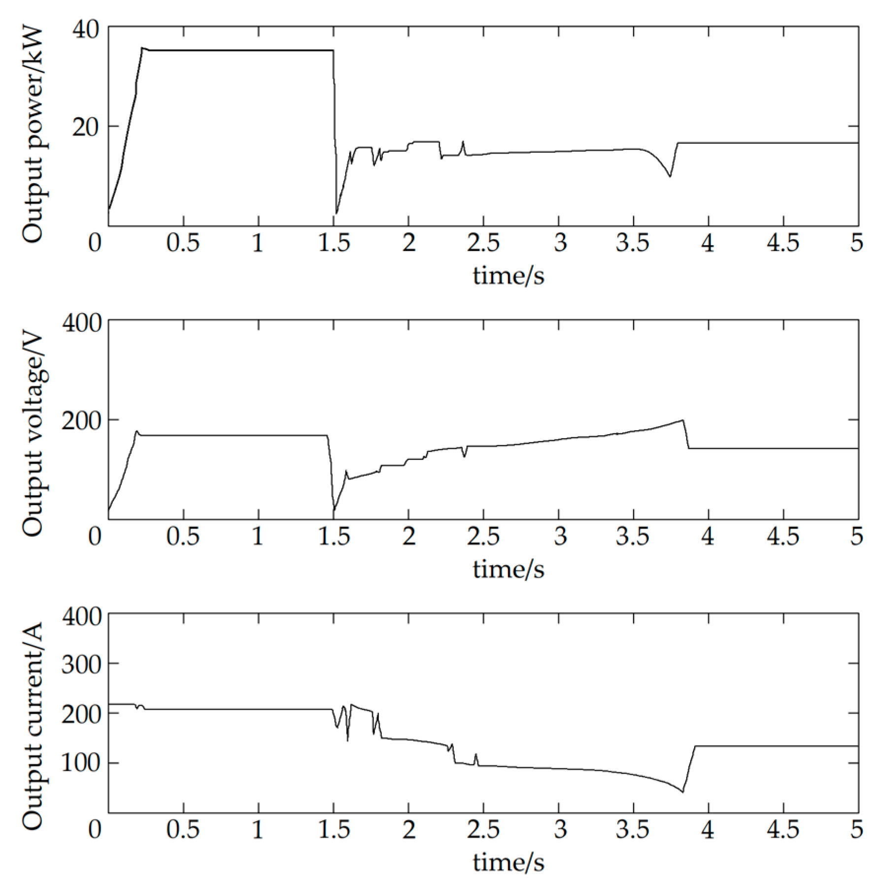
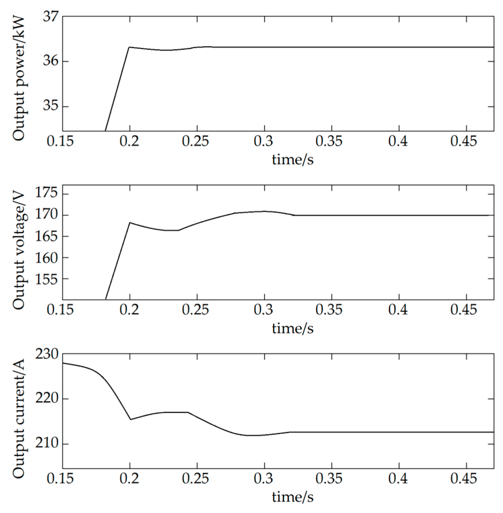
Tandem PV arrays are used as simulation objects, with the number of tandem arrays at thirty, each group of tandem PV arrays consisting of ten modules in tandem, of which four modules are in the normal light environment and six modules are in the shadow state, and the light intensity of the PV arrays at 300 W/m2. In the simulation, Fibonacci searches for the subroutine to set the relative accuracy to 0.05 and the absolute accuracy to 1. In the simulation, the PV square array starts with uniform illumination as the starting environment. At t = 1.5 s, when the PV array is in a complex lighting environment, the simulation results of the maximum power point tracking of the PV array are shown in Figure 6, which are the real-time change curves of the output power, output voltage, and output current, respectively, and the enlarged diagram of the tracking curve in Figure 6 from 0.15 to 0.45 s, i.e., the maximum power tracking curve of the PV array under the uniform illumination environment, is shown in Figure 7 [25], showing, respectively, from top to bottom, output power, output voltage, and output current.
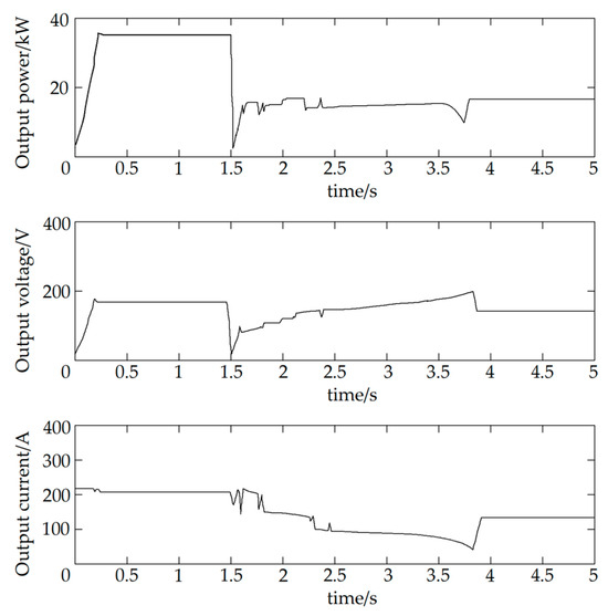
Figure 6.
Simulation curve of maximum power tracking algorithm under shadow conditions.
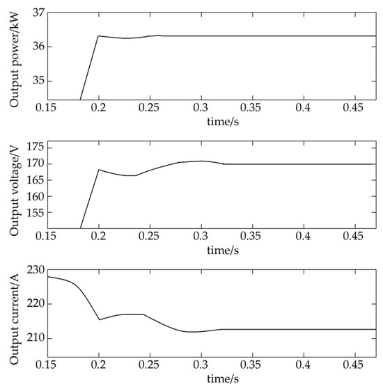
Figure 7.
Maximum power tracking curve of photovoltaic array under uniform illumination environment.
The search starts at t = 0 s, and the operating voltage of the PV array immediately rises to 170 V. The system determines that the PV array is currently in an even-light environment and calls the Fibonacci search algorithm, which tracks the maximum output power of the PV array at t = 0.2 s and ends the tracking at t = 0.32 s. The operating voltage of the PV array is about 169.85 V and the output power is about 37.25 kW. The tracking procedure is resumed when the time reaches 1.5 s. The output power of the PV array decreases to 12.5 kW when the output voltage rises to 85 V. The system detects that the PV array is in a complex lighting environment, and in order to track the PV array’s peak power in each voltage range, a Fibonacci search subroutine is used [26]. At t = 2.4 s, the output voltage of the PV array is 153 V, and the system initiates the variable step-size perturbation observation method until the end of tracking at t = 3.8 s, at which point the peak power of the PV array is tracked. The rated operating voltage of the PV array is 120 V, and the maximum output power is 17 kW.
6. Simulation Based on Improved Fibonacci Linear Search Algorithm
For the controller, the algorithm, the Fibonacci linear search method, has two outstanding advantages: easy adjustment of control parameters and fast response speed. This MPPT technique for PV power systems based on the modified Fibonacci linear search algorithm is capable of tracking the maximum power point under non-consistent insolation or drastic changes in insolation. The modified Fibonacci search algorithm is applicable to time-varying P-V characteristic curves. When the insolation changes drastically, a new initialization function is introduced to initialize the search conditions and do a wide-range search to obtain the actual maximum power.
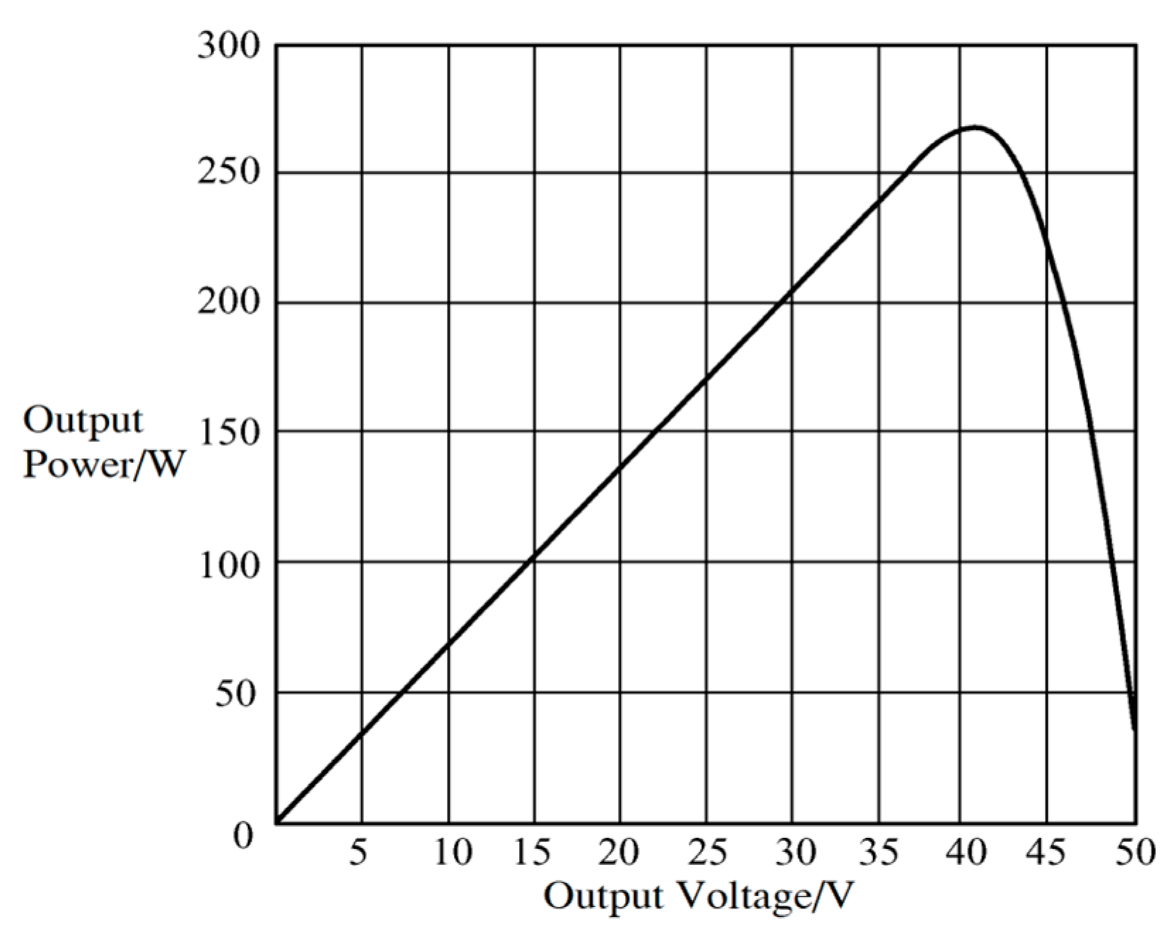
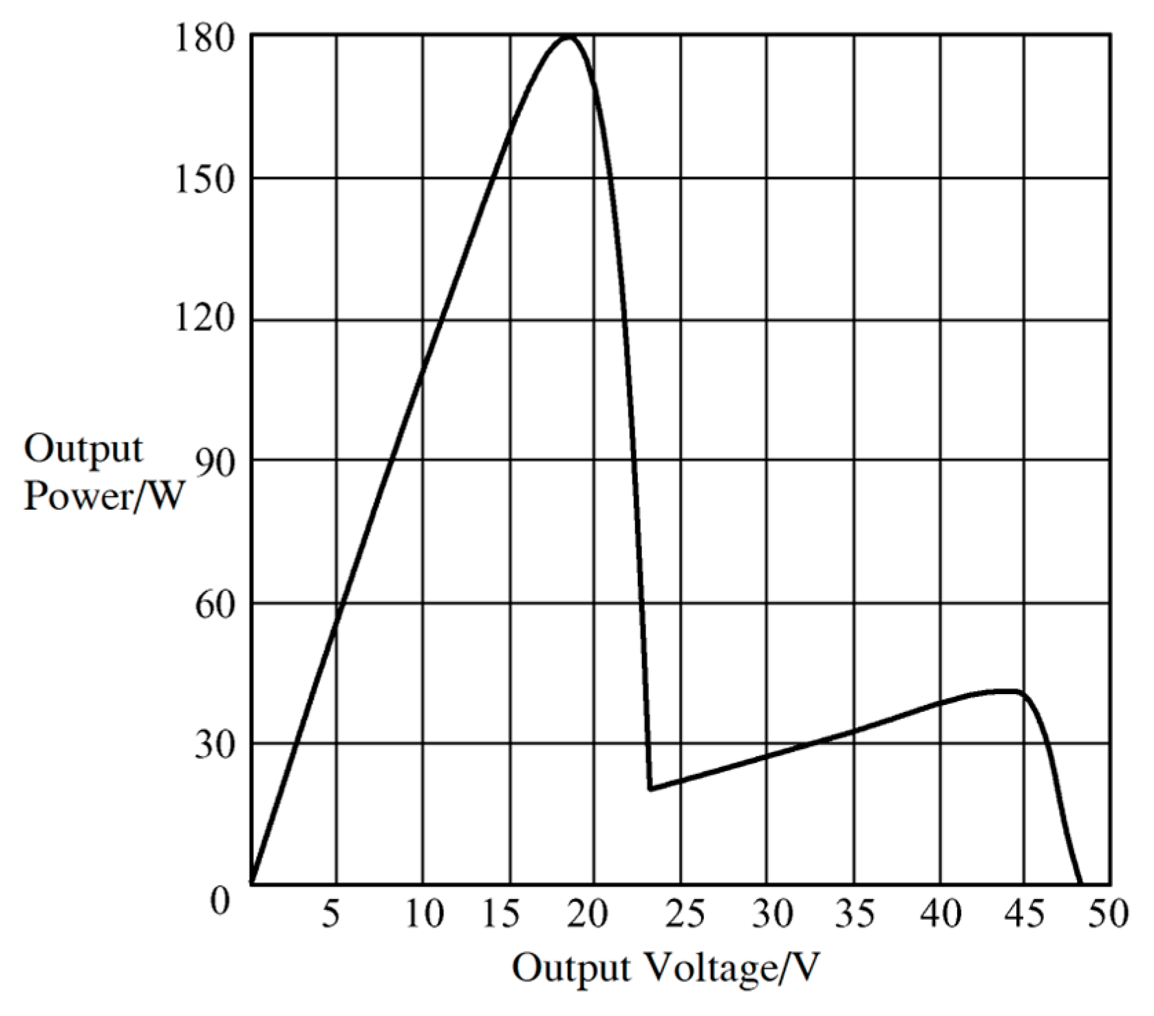
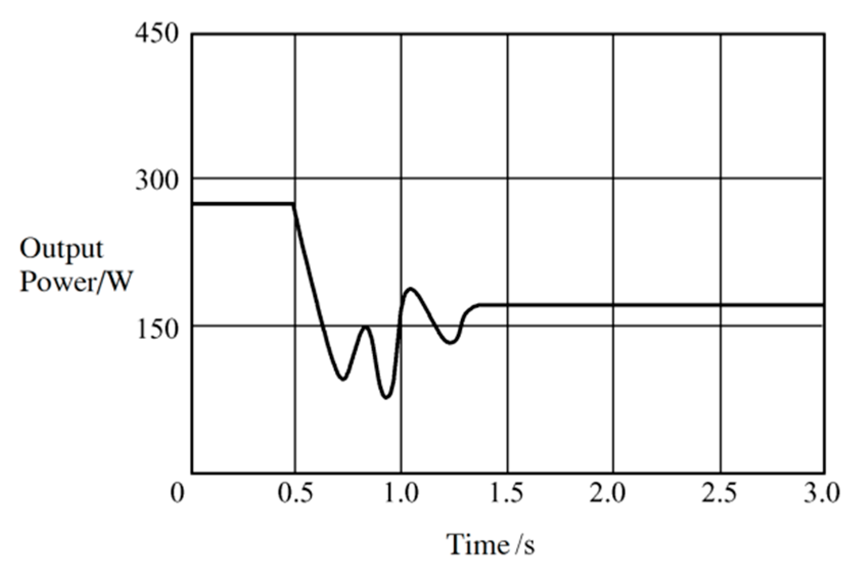
The photovoltaic module consists of 36 cells with a rated output power of 140 W, an open circuit voltage of 25.5 V, and a short circuit current of 7.85 A. Each cell has an area of 0.0225 m2, Rs = 0.006 Ω, and Rsh = 10,000 Ω. Two modules are connected in series with an anti-reverse charge diode. The assembly was found to meet the production specifications and ideal requirements for the operating temperature (T = 320 K). In order to simulate the variation in insolation conditions, it is assumed that the intensity of insolation radiation on both assemblies is S = 1000 W/m2 at t = 0. When the time t is 0.5 s, the intensity of insolation radiation on both assemblies is S = 1000 W/m2 and S = 100 W/m2, respectively, and the simulation results are shown in Figure 8, Figure 9 and Figure 10 [27].
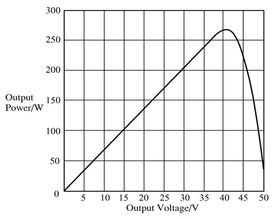
Figure 8.
P-V simulation curves of the module with no change in solar radiation conditions.
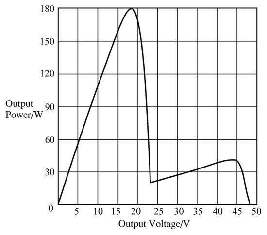
Figure 9.
P-V simulation curve of the component when partial occlusion occurs.
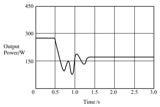
Figure 10.
Simulated waveforms of MPPT output power based on Fibonacci algorithm.
From Figure 8, it can be seen that when the PV module is shaded for some reason, which changes the insolation radiation, the system has two extremes at two different voltage values of 18 V and 44 V for the output voltage, but the former is significantly higher than the latter, and a local maximum point occurs. The MPPT control method using the Fibonacci algorithm enables a global search to track the actual maximum power point without the loss of energy due to operating at the local maximum power point [28]. Figure 10 shows the output power simulation waveforms using the MPPT control method based on the modified Fibonacci search algorithm, and the global maximum power point of the system can be observed to be around 180 W under the localized shading condition.
7. Simulation Experiment Analysis
In this paper, the basic principle and flow chart of the improved MPPT algorithm are introduced, and the improved MPPT algorithm is simulated to verify its tracking effect. The simulation circuit is built based on PSIM9.0, the PV cell model adopts the physical model of the battery module that comes with PSIM, which has two interfaces, S and T, at the input side, and the light intensity and cell temperature are simulated by using specific voltage values. The model has a maximum power output port at the top, which allows real-time monitoring of the maximum power of the PV cell in the current environment.
The detailed specifications of PSIM’s built-in photovoltaic module are as follows:
(1) Basic performance indicators
The basic performance indicators are shown in Table 5.
Table 5.
Default configuration table.
(2) Physical characteristic parameters.
Number of battery cells: default 36 in series (modifiable).
Battery area: 0.0225 m2/piece (customizable).
Ideal factor (n): 1.2 (range 1.0–2.0).
Series resistance (Rs): 0.006 Ω (range 0–1 Ω).
Parallel resistance (Rsh): 10,000 Ω (range 100–100 kΩ).
The DLL module is required for the implementation of simulation control, and it is only necessary to put the DLL module into the dll file location of the program. The simulation effect is shown in Figure 11.
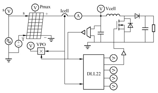
Figure 11.
MPPT model simulation.
The photovoltaic module is made of 36 polycrystalline silicon photovoltaic cells so that the temperature is constant at 25 °C, the solar radiation intensity period is 0.02 s, and the duty cycles of 1100 W/m2 and 500 W/m2 are each 0.5.
Considering the number of photovoltaic cells, the output characteristic equation is
In the formula, Ns is the number of battery cells, the exponent numerator q (U + NsrsI) represents the total voltage drop of the component (including the series resistance voltage drop), and the denominator Nsnkt distributes the voltage to the single-cell level to calculate the PN junction characteristics.
The following is a comparative analysis of five key parameters of photovoltaic modules in PSIM simulation and typical literature data.
(1) Number of photovoltaic modules
The comparative analysis between the default value of photovoltaic module number in PSIM and the typical values in the literature is shown in Table 6.
Table 6.
Comparative analysis of the number of photovoltaic modules.
(2) Temperature
The comparative analysis between the default values of temperature in PSIM and the measured data in literature is shown in Table 7.
Table 7.
Temperature comparison analysis.
(3) Sunshine radiation intensity cycle
The comparative analysis between the PSIM example values of sunshine radiation intensity cycle and the experimental data in the literature is shown in Table 8.
Table 8.
Comparative analysis of sunshine radiation intensity cycles.
(4) Light intensity
The comparative analysis between the PSIM range of light intensity and the literature data range is shown in Table 9.
Table 9.
Comparative analysis of light intensity.
(5) Duty cycle
The comparative analysis between the PSIM MPPT output values of duty cycle and the optimization results is shown in Table 10.
Table 10.
Comparative analysis of duty cycle.
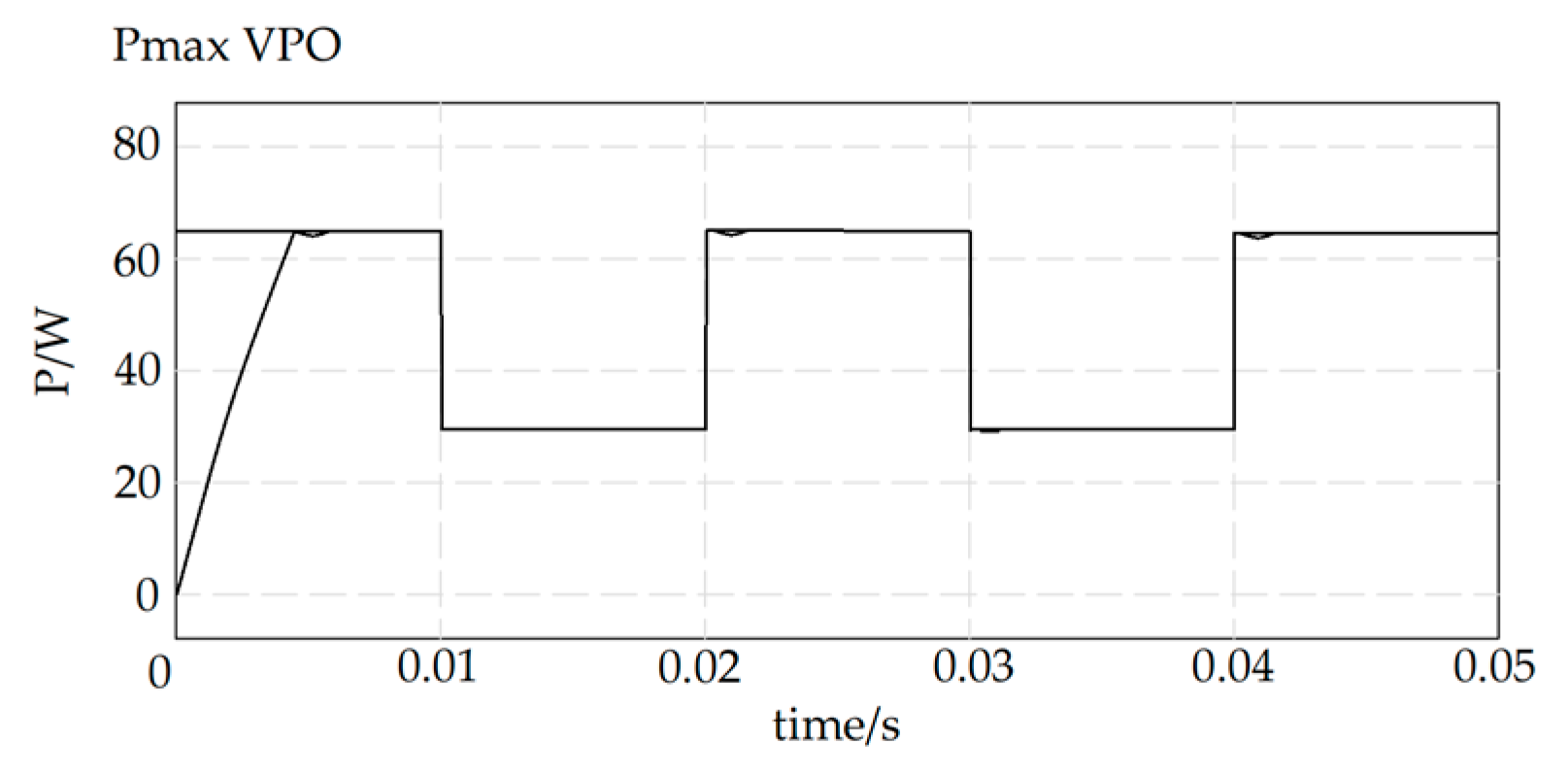
The simulation results are shown in Figure 12.
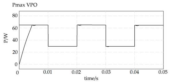
Figure 12.
Simulation results of MPPT algorithm.
From Figure 12, the MPPT algorithm takes 5 ms to track the maximum power point of the PV module at the beginning of the operation, while the MPPT can quickly and accurately realize the tracking of the maximum power point when the external lighting conditions change, which is very satisfactory [29].
8. Conclusions
This article is based on the improved Fibonacci linear search algorithm for MPPT design, which has certain innovative advantages, but there are still some issues that need further in-depth research.
Innovation advantages:
(1) Core innovation at the algorithm level based on the fusion of dual precision termination conditions
① Traditional method: relying solely on interval relative accuracy δ;
② Improvement plan: introduce dual criteria for absolute power accuracy ε;
③ Effect: avoid oscillation near the maximum power point;
④ The response speed has been significantly improved compared to traditional methods.
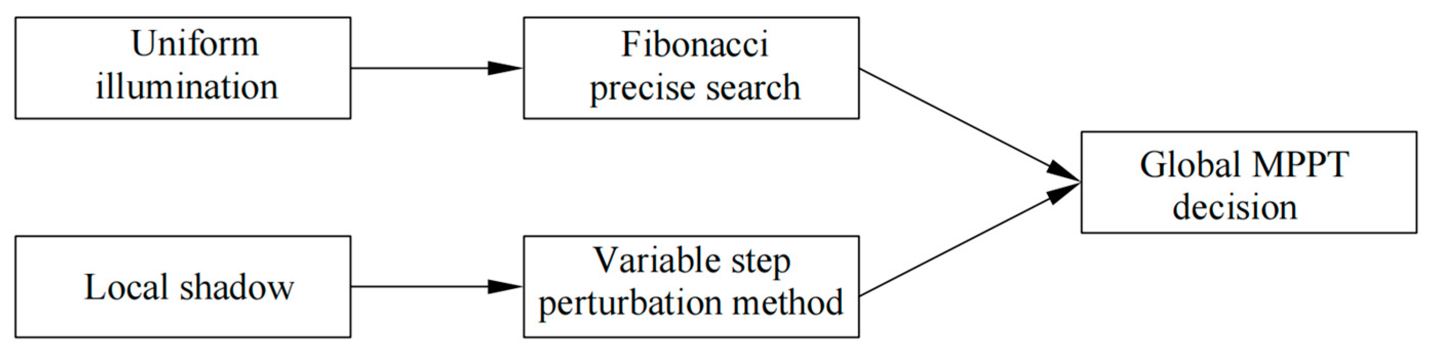
(2) System architecture innovation
The system architecture innovation is shown in Figure 13.
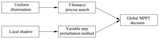
Figure 13.
Hybrid tracking strategy diagram.
(3) Performance improvement verification
The comparison of performance improvements for each indicator is shown in Table 11.
Table 11.
Performance improvement data sheet.
(4) Comparison to existing technological advantages
① Compared to the perturbation observation method: reduced power fluctuations;
② Compared to the incremental conductivity method: reduced computational complexity;
③ Compared to traditional Fibonacci, the success rate of global MPPT under shadow conditions has been improved.
Future research directions and prospects:
(1) Improve the efficiency of the algorithm: At present, although the improved Fibonacci linear search algorithm has high accuracy and convergence speed, it still has the problem of high computational complexity when dealing with large-scale PV arrays. Therefore, future research can explore how to further improve the efficiency of the algorithm to adapt to larger-scale PV arrays.
(2) Considering multiple lighting conditions: The existing improved Fibonacci linear search algorithm is mainly optimized for MPPT control under constant lighting conditions. However, in actual operation, PV arrays may be affected by multiple light conditions, such as sunrise, sunset, and cloud cover. Therefore, future research can explore how to incorporate these factors into the algorithm model to improve the adaptability and robustness of the algorithm.
(3) Combining other control strategies: In addition to the improved Fibonacci linear search algorithm, there are many other MPPT control strategies to choose from, such as the perturbation observation method, the incremental conductance method, and so on. Future research can explore how to combine different control strategies into MPPT control to obtain more accurate and efficient results [30].
(4) Considering the grid access problem: With the popularization and development of distributed generation technology, more and more PV power systems need to be connected to the grid. Therefore, future research can explore how to ensure the performance of MPPT while realizing the stable grid-connected operation of PV power generation systems.
Author Contributions
Conceptualization, Z.M., Y.S. and X.Y.; methodology, Z.M., Y.S. and X.Y.; software, Z.M. and X.Y.; writing—original draft, Z.M., Y.S. and X.Y. All authors have read and agreed to the published version of the manuscript.
Funding
This study was supported by the “Teaching Leading Talents” project of the Shaanxi Sanqin Talent Special Support Program (funder: Shaanxi Provincial Department of Education), the Shaanxi Provincial “14th Five Year Plan” Education Science Planning Project SGH23Q0397 (funder: Shaanxi Provincial Department of Education), the Chongqing Natural Science Foundation Project CSTB2022NSCQ-MSX0574 (funder: Chongqing Science and Technology Bureau), and the Qin Chuangyuan High level Innovation and Entrepreneurship Talent Project QCYRCXM-2022-306 (funder: Shaanxi Provincial Department of Science and Technology).
Data Availability Statement
The original contributions presented in this study are included in the article. Further inquiries can be directed at the corresponding authors.
Conflicts of Interest
Author Zhuo Meng was employed by Shaanxi Energy Institute. The remaining authors declare that the research was conducted in the absence of any commercial or financial relationships that could be construed as a potential conflict of interest. The institute had no role in the design of the study; in the collection, analyses, or interpretation of data; in the writing of the manuscript, or in the decision to publish the results.
References
- Wei, X. Photovoltaic Power Generation Technology and Its Application; Machinery Industry Press: Beijing, China, 2022; pp. 133–164. [Google Scholar]
- Esram, T.; Chapman, P.L. Comparison of Photovoltaic array maximum power point tracking techniques. IEEE Trans. Energy Convers. 2007, 22, 439–449. [Google Scholar] [CrossRef]
- Duman, S.; Yorukeren, N.; Altas, I.H. A novel MPPT algorithm based on optimized artifieial neural network by using FPSOGSA for standalone photovoltaic energy systems. Neural Comput. Appl. 2018, 29, 257–278. [Google Scholar] [CrossRef]
- Roy, R.B.; Rokonuzzaman, M.; Amin, N.; Mishu, M.K.; Alahakoon, S.; Rahman, S.; Mithulananthan, N.; Rahman, K.S.; Shakeri, M.; Pasupuleti, J. A comparative performance analysis of ANN al-gorithms for MPPT energy harvesting in solar PV system. IEEE Access 2021, 9, 102137–102152. [Google Scholar] [CrossRef]
- Khan, M.J.; Pushparaj. A novel hybrid maximum power point tracking controller based on artificial intelligence for solar photovoltaic system under variable environmental conditions. J. Electr. Eng. Technol. 2021, 16, 1879–1889. [Google Scholar] [CrossRef]
- Fathi, M.; Parianj, A. Intelligent MPPT for pho-tovoltaic panels using a novel fuzzy logic and artificial neural networks based on evolutionary algorithms. Energy Rep. 2021, 7, 1338–1348. [Google Scholar] [CrossRef]
- Jyothy, L.P.N.; Sindhu, M.R. An Artificial Neural Network Based MPPT Algorithm for Solar PV System. In Proceedings of the International Conference on Electrical Energy Systems, Chennai, India, 7–9 February 2018; pp. 375–380. [Google Scholar]
- Windarko, N.A.; Nizar Habibi, M.; Sumantri, B.; Prasetyono, E.; Efendi, M.Z.; Taufik. A new MPPT algorithm for photovoltaic power generation under uniform and partial shading conditions. Energies 2021, 14, 483. [Google Scholar] [CrossRef]
- Kalogerakis, C.; Koutroulis, E.; Lagoudakis, M.G. Global MPPT based on machine-learning for PV arrays operating under partial shading conditions. Appl. Sci. 2020, 10, 700. [Google Scholar] [CrossRef]
- Hassan, T.U.; Abbassi, R.; Jerbi, H.; Mehmood, K.; Tahir, M.F.; Cheema, K.M.; Elavarasan, R.M.; Ali, F.; Khan, I.A. A novel algorithm for MPPT of an isolated PV system using push pull converter with fuzzy logic controller. Energies 2020, 13, 4007. [Google Scholar] [CrossRef]
- Liu, X.; Lopes, L.A. An Improved Perturbation and Observation Maximum Power Point Tracking Algorithm for PV Arrays. In Proceedings of the IEEE 35th Annual Meeting of Power Electronics Specialists Conference, Aachen, Germany, 20–25 June 2004. [Google Scholar]
- Kheldoun, A.B.; Bradai, R.; Boukenoui, R.; Mellit, A. A new Golden Section method-based maximum power point tracking algorithm for photovoltaic systems. Energy Convers. Manag. 2016, 111, 125–136. [Google Scholar] [CrossRef]
- Irmak, E.; Güler, N. A model predictive control-based hybrid MPPT method for boost converters. Int. J. Electron. 2020, 107, 1–16. [Google Scholar] [CrossRef]
- Swaminathan, N.; Lakshminarasamma, N.; Cao, Y. A fixed zone perturb and observe MPPT technique for A standalone distributed PV system. IEEE J. Emerg. Sel. Top. Power Electron. 2022, 10, 361–374. [Google Scholar] [CrossRef]
- Fu, C.X.; Zhang, L.X.; Dong, W.C. Research and application of mppt control strategy based on improved slime mold algorithm in shaded conditions. Electronics 2022, 11, 2122. [Google Scholar] [CrossRef]
- Abdalla, O.; Rezk, H.; Ahmed, E.M. Wind driven optimization algorithm based global MPPT for PV system under non-uniform solar irradiance. Sol. Energy 2019, 180, 429–444. [Google Scholar] [CrossRef]
- Guenounou, O.; Dahhou, B.; Chabour, F. Adaptive fuzzy controller based MPPT for photovoltaic systems. Energy Convers. Manag. 2014, 78, 843–850. [Google Scholar] [CrossRef]
- Rezk, H.; Aly, M.; Al-Dhaifallah, M.; Shoyama, M. Design and hardware implementation of new adaptive fuzxy logic- based MPPT control method for photovoltaic applications. IEEE Access 2019, 7, 106427–106438. [Google Scholar] [CrossRef]
- Tey, K.S.; Mekhilef, S.; Seyedmahmoudian, M.; Horan, B.; Oo, A.T.; Stojcevski, A. Improved differential evolution-based MPPT algorithm using SEPIC for PV systems under partial shading conditions and load variation. IEEE Trans. Ind. Inform. 2018, 14, 4322–4333. [Google Scholar] [CrossRef]
- Bollipo, R.B.; Mikkili, S.; Bonthagorla, P.K. Hybrid, optimal, intelligent and classical PV MPPT techniques: A review. CSEE J. Power Energy Syst. 2021, 7, 9–33. [Google Scholar]
- Amara, K.; Malek, A.; Bakir, T.; Fekik, A.; Azar, A.T.; Almustafa, K.M.; Bourennane, E.B.; Hocine, D. Adaptive neurofuzxy inference system based maximum power point tracking for stand-alone photovoltaic system. Int. J. Model. Identif. Control 2019, 33, 311. [Google Scholar] [CrossRef]
- Ali, M.N.; Mahmoud, K.; Lehtonen, M.; Darwish, M.M. An efficient fuzzy-logic based variable-step incremental conductance MPPT method for grid-connected PV systems. IEEE Access 2021, 8, 26420–26430. [Google Scholar] [CrossRef]
- Zhang, J.H.; Wei, X.Y.; Hu, L.; Ma, J.G. A MPPT method based on improved Fibonacci search photovoltaic array. Tech. Gaz. 2019, 26, 163–170. [Google Scholar]
- Yadav, V.K.; Jha, S.K.; Kumar, B. Comparative Study of Different Variable Step Size Perturb and Observe Based MPPT. In Proceedings of the 2020 Intemational Conference on Advances in Computing, Communication & Materials, Dehradun, India, 21–22 August 2020; pp. 272–277. [Google Scholar]
- Ali, Z.M.; Quynh, N.V.; Dadfar, S.; Nakamura, H. Variable step size perturb and observe MPPT controller by applying θ-modified krill herd algorithm-sliding mode controller to increase accuracy in photovoltaic system. J. Clean. Prod. 2020, 271, 122243. [Google Scholar] [CrossRef]
- Ge, X.; Ahmed, F.W.; Rezvani, A.; Aljojo, N.; Samad, S.; Foong, L.K. Implementation of a novel hybrid BAT-fuzzy controller based MPPT for grid-connected PV-battery system. Control Eng. Pract. 2020, 98, 104380. [Google Scholar] [CrossRef]
- Ahmed, J.; Salam, Z. An enhanced adaptive P&Q MPPT for fast and efficient tracking under varying environmental conditions. IEEE Trans. Sustain. Energy 2018, 3, 1487–1496. [Google Scholar]
- Çırak, C.R.; Çalık, H. Hotspots in maximum power point tracking algorithms for photovoltaic systems A Comprehensive and Comparative review. Eng. Sci. Technol. Int. J. 2023, 43, 101436. [Google Scholar] [CrossRef]
- Verma, A.; Yadav, S.; Arora, A.; Singh, K. Comparison of Maximum Power Tracking Using Artificial Intelligence Based Optimization Controller in Photovoltaic Systems. In Proceedings of the 2020 International Conference for Emerging Technology, Belgaum, India, 5–7 June 2020; pp. 1–6. [Google Scholar]
- Tang, L.; Wang, X.; Xu, W.; Mu, C.; Zhao, B. Maximum power point tracking strategy for photovoltaic system based on fuzzy information diffusion under partial shading conditions. Sol. Energy 2021, 220, 523–534. [Google Scholar] [CrossRef]


Disclaimer/Publisher’s Note: The statements, opinions and data contained in all publications are solely those of the individual author(s) and contributor(s) and not of MDPI and/or the editor(s). MDPI and/or the editor(s) disclaim responsibility for any injury to people or property resulting from any ideas, methods, instructions or products referred to in the content. |
© 2025 by the authors. Licensee MDPI, Basel, Switzerland. This article is an open access article distributed under the terms and conditions of the Creative Commons Attribution (CC BY) license (https://creativecommons.org/licenses/by/4.0/).