A Lightweight Multi-Scale Object Detection Framework for Shrimp Meat Quality Control in Food Processing

Abstract

Reliable quality and size inspection of shrimp meat is essential in food processing to ensure food safety, enhance production efficiency, and promote sustainable practices. However, significant scale differences in shrimp meat categories and the presence of subtle local defects pose challenges to traditional manual inspection methods, resulting in low efficiency and high rates of false positives and negatives. To address these challenges, we propose a lightweight multi-scale object detection framework specifically designed for automated shrimp meat inspection in food processing environments. Our framework incorporated a novel downsampling module (ADown) that was engineered to reduce parameters while preserving essential features. Additionally, we propose dual-scale information selection convolution (DSISConv), multi-scale information selection convolution (MSISConv), and a lightweight multi-scale information selection detection head (LMSISD) to improve detection accuracy across diverse object scales. Furthermore, a bidirectional complementary knowledge distillation strategy was employed, which enabled the lightweight model to learn crucial features from a larger teacher model without increasing inference complexity. Experimental results validated the effectiveness of our approach. Compared to the YOLOv11n (baseline) model, the proposed framework improved precision by 1.0%, recall by 0.8%, mAP50 by 0.9%, and mAP50-95 by 1.3%, while simultaneously reducing parameters by 7.1%, model size by 8.0%, and GFLOPs by 22.2%. The application of knowledge distillation yielded further improvements of 0.1% in precision, 1.2% in recall, 0.5% in mAP50, and 0.5% in mAP50-95. These results indicated that the proposed approach provided an effective and efficient solution for real-time shrimp meat inspection, balancing high accuracy with low computational requirements.

1. Introduction

Aquaculture, a vital component of the global food supply, has recently exceeded capture fisheries in production for the first time [1]. Within the rapidly growing aquaculture sector, shrimp farming stands out due to its high economic value and expanding production scale. China leads in global shrimp production, experiencing substantial growth over the past two decades [2]. However, this growth poses challenges for maintaining quality during processing. With rising production levels and consumer demands for quality, ensuring the safety and quality of shrimp products along the supply chain is now a critical concern for processing firms. Detecting and categorizing quality defects in processed shrimp products efficiently is particularly complex and necessitates innovative technical solutions.

Despite advancements in technology, many processing facilities continue to utilize a mix of automated machinery and manual techniques for detecting defects and classifying specifications in shrimp meat. This traditional approach encounters significant challenges when addressing a variety of shrimp quality defects across different scales and categories, including dehydration, discoloration, physical damage, incomplete removal of shells, inadequate cleaning of intestinal glands, and the presence of mixed shell fragments. These challenges pose a threat to the industry’s sustainability by compromising food safety, diminishing production efficiency, and inflating operational costs.

• Ensuring the accuracy and consistency of detection in artificial vision systems poses challenges due to reliance on experiential and subjective judgment. Factors such as fatigue can compromise detection rates and consistency, potentially resulting in substandard products reaching the market. This situation not only jeopardizes consumer health but also undermines the company’s reputation and brand value.
• As production expands, repetitive labor-intensive tasks lead to heightened labor costs and administrative complexities. The escalating labor expenses in today’s economic landscape directly erode enterprises’ profit margins and competitive edge.
• The substantial variations in characteristic scales among various shrimp categories, coupled with their nuanced local defects, contribute to diminished detection efficacy and elevated rates of false positives and false negatives for operators. These challenges not only compromise product quality uniformity but also hamper production line efficiency, rendering it inadequate to meet the demands of large-scale processing. Consequently, this scenario impacts production output and market supply capacity for enterprises.

To address these limitations, academia and industry are actively exploring advanced detection technologies to replace or supplement manual methods.

Traditional methods with manual feature extraction were the initial focus of early research. Lee et al. [3] utilized the turning angle distribution analysis (TADA) algorithm to distinguish between intact and damaged shrimp. Zhang et al. [4] extended this by proposing evolutionary constructed (ECO) features combined with AdaBoost classifiers. Their system achieved an overall classification accuracy of 95.1%, precision of 0.948, and recall of 0.920 in experimental evaluations.

Machine learning methodologies subsequently superseded purely manual approaches. Liu et al. [5] conducted comparative analyses of traditional machine learning algorithms (KNN, SVM, BP neural networks) and achieved significant accuracy in shrimp identification. Zhou et al. [6] developed SLCNet based on density map regression for shrimp fry quantification and dimensional assessment. However, these methodologies, dependent on shallow architectures or handcrafted features, demonstrated inherent limitations when processing multi-scale targets, complex environmental backgrounds, and morphological variations, failing to optimize the accuracy-robustness equilibrium.

Deep learning-based detection methodologies have transformed this research domain in recent years. Catalyzed by the advancement of convolutional neural networks (CNNs), deep learning architectures for object detection and classification have gained prominence in aquatic product inspection systems. Hu et al. [7] introduced ShrimpNet, implementing a simplified CNN architecture for diverse shrimp species identification. Liu et al. [8] engineered Deep-ShrimpNet based on modified AlexNet architecture, demonstrating high-precision detection capabilities. Nevertheless, these neural architectures exhibit performance constraints when deployed in complex shrimp processing environments. Industrial applications characterized by multiple defect categories, significant scale variations, and cluttered backgrounds necessitate models with enhanced feature extraction and generalization capacities.

Among deep learning methodologies, YOLO (you only look once)-based frameworks have become mainstream in object detection due to their optimal speed–accuracy balance. Researchers have modified the baseline YOLO architecture to enhance performance for multi-scale object detection.

Several YOLO variants target small-object detection challenges. Tian et al. [9] developed MD-YOLO for small-pest detection with good accuracy, but suffered from large parameter counts (126.8 MB), extended training times, and detection failures in complex backgrounds. Tao et al. [10] engineered EFE-YOLO with pixel shuffle and receptive field attention modules, improving accuracy while reducing detection speed from 72.7 to 61.0 FPS. Li et al. [11] introduced DMA-YOLO for aerial imagery, enhancing small-object detection, but decreasing inference speed from 63.29 to 31.11 FPS, limiting its real-time applications.

Other YOLO variants address diverse application domains. Cao et al. [12] proposed MCS-YOLO for autonomous driving, improving accuracy, but increasing computational demands and reducing inference speed. Wang and Hao [13] developed YOLO-SK, a lightweight algorithm that maintained low parameter counts, but showed poor adaptability in complex scenes and high noise sensitivity. Additional studies by Wang et al. [14], Guo et al. [15], Peng et al. [16], Su et al. [17], and Li et al. [18] presented YOLO variants for specific applications, yet faced persistent trade-offs between computational efficiency and detection performance.

The literature review identifies significant shortcomings in current methods for assessing shrimp meat quality. Traditional techniques relying on manual feature extraction struggle with complex backgrounds and multi-scale targets. Although deep learning methods show promise, existing CNN architectures lack the necessary feature representation for diverse shrimp defects. While YOLO-based frameworks enhance detection accuracy, they face a trade-off: high-precision models like MD-YOLO, EFE-YOLO, and DMA-YOLO demand substantial computational resources and operate slowly, whereas lightweight models such as YOLO-SK underperform in intricate settings. This underscores the need for models that can achieve high-precision detection of multi-scale defects with limited computational resources while maintaining real-time capabilities. To address these challenges, we propose the ADL-YOLO lightweight multi-scale detection model.

In order to fill critical knowledge voids in the advancement of models capable of concurrently achieving precise multi-scale defect detection, real-time performance, and efficient operation within constrained computational resources, we introduce ADL-YOLO, a streamlined multi-scale object detection model. Our primary objective is to surmount the accuracy–efficiency trade-offs constraining current YOLO-based approaches, particularly in the context of detecting multi-scale, diverse quality defects and sizing shrimp meat. The key technological advancements of this investigation can be outlined as follows.

• The ADown module is an innovative downsampling method that substitutes conventional convolution, maintaining essential features while decreasing parameters and computational expenses.
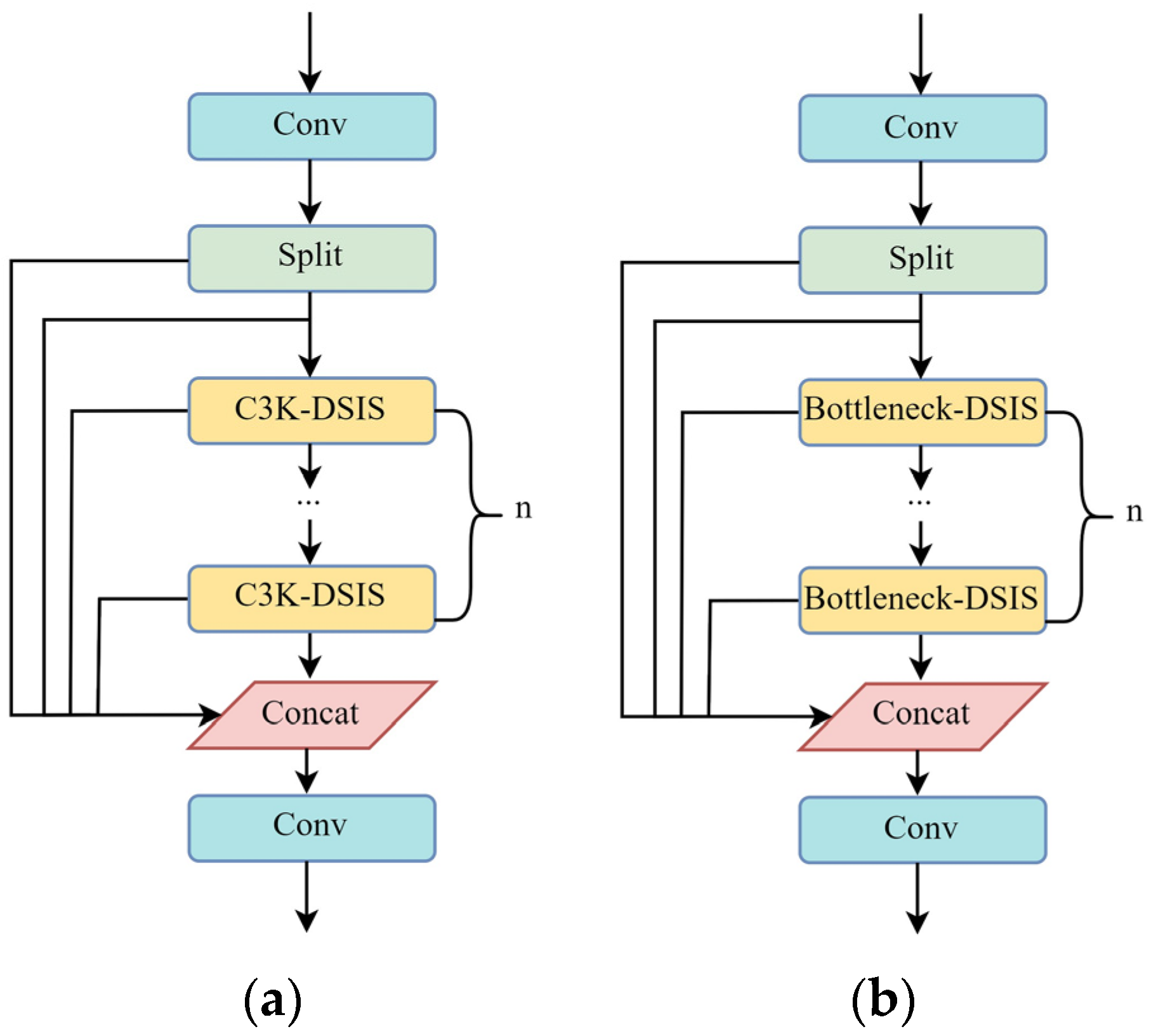
• DSISConv and MSISConv are convolutional methods that selectively incorporate information at two scales and multiple scales, respectively. DSISConv is combined with C3K2 to create C3K2–DSIS, enhancing adaptive multi-scale feature extraction for enhanced detection of defects across varying sizes.
• The LMSISD detector head, based on MSISConv, integrates multi-scale feature fusion and lightweight network design to enhance detection performance.
• Bidirectional knowledge distillation is an enhanced method of distillation that facilitates lightweight student models in acquiring crucial features from teacher models, leading to high accuracy while maintaining minimal parameter complexity.

This research offers an efficient solution for shrimp meat quality inspection. It also presents new techniques for lightweight detection systems in other food safety domains. We bridge the gap between advanced algorithms and real-world needs. Our approach improves food safety, reduces computational demands, and supports sustainable processing practices.

2. Related Works

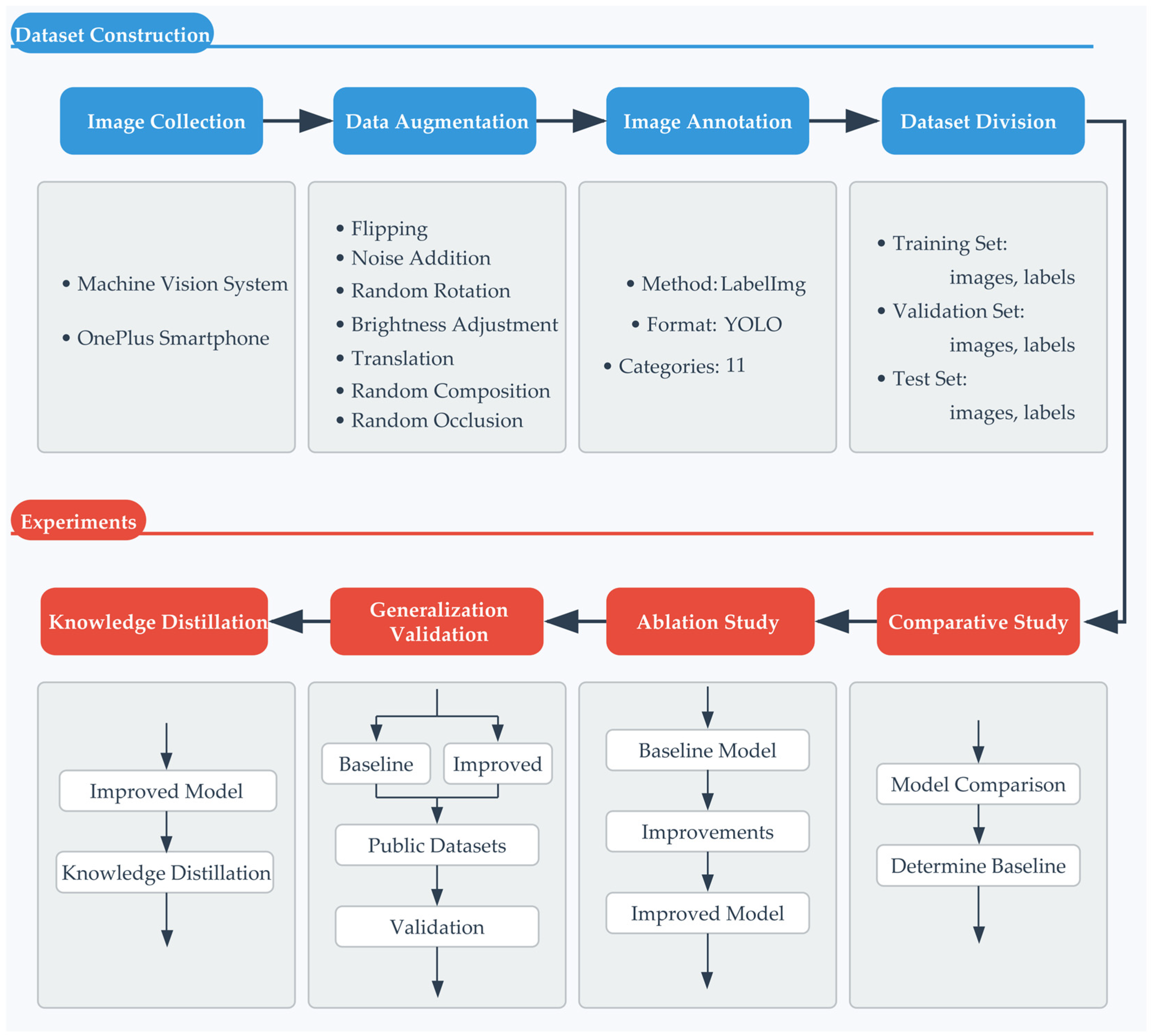
2.1. Experimental Workflow Overview

This study followed a systematic technical approach encompassing data acquisition, model refinement, and validation, as depicted in Figure 1. Initially, shrimp meat sample images were captured using a machine vision system and a OnePlus Ace2 smartphone (OPPO, Shenzhen, China) to gather raw data from various perspectives and backgrounds. Subsequently, the data underwent enhancement procedures, such as inversion, random angle rotation, brightness adjustment, translation, noise addition, random occlusion, and random combination, to bolster the model’s robustness and generalization capabilities. The LabelImg tool was utilized to annotate samples across 11 categories in YOLO format, with the dataset partitioned into training, validation, and test subsets at an 8:1:1 ratio.

In the experimental phase, the foundational model was established through comparative experiments, followed by further evaluations through contrast and ablation experiments to assess the efficacy of each enhanced module. The model’s generalization capacity was validated using publicly available datasets. Subsequently, a bidirectional complementary knowledge distillation approach was implemented to enhance the model’s performance. The entire research process adhered to a systematic technical pathway spanning from data acquisition to model development, from foundational establishment to optimization, with the objective of addressing the challenge of multi-scale target detection in shrimp meat quality assessment. Having established the overall experimental workflow, the next section details the specific experimental materials used in this study.

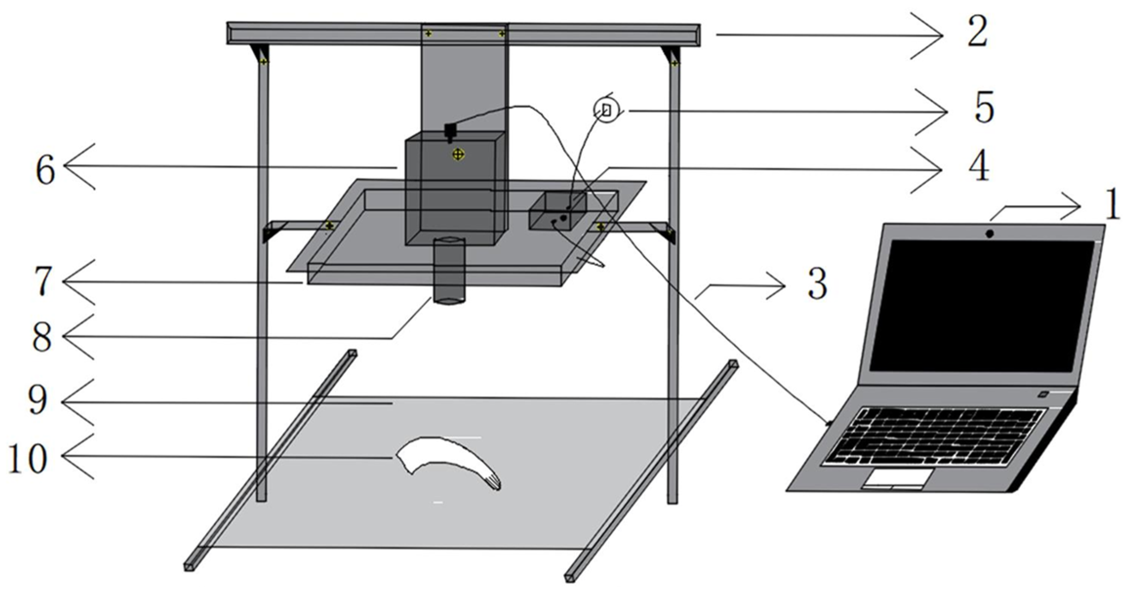
2.2. Experimental Materials

This section provides a detailed account of the dataset construction process, outlining the steps involved in sample image acquisition, data augmentation, data labeling, and dataset partitioning.

The experimental materials used in this study were Pacific white shrimp (Litopenaeus vannamei) meat samples. The samples were collected from Huazhou Dianshuo Aquatic Science and Technology Co., Ltd., located in Maoming, Guangdong Province, China (21°31′ N, 110°36′ E). Sampling occurred between October and early November 2024 during the hours of 08:00 to 17:00 daily. Samples were randomly collected from three to five different production batches across three daily time periods: morning (08:00–11:00), midday (11:00–14:00), and afternoon (14:00–17:00), with approximately 20–50 specimens obtained during each sampling session. Based on morphological characteristics and processing requirements, the shrimp meat samples were categorized into three primary groups and eleven subcategories (detailed in Figure 2):

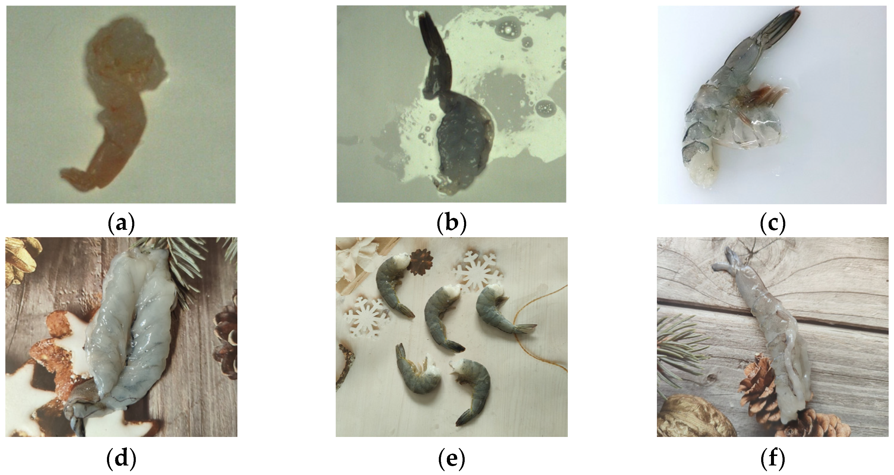
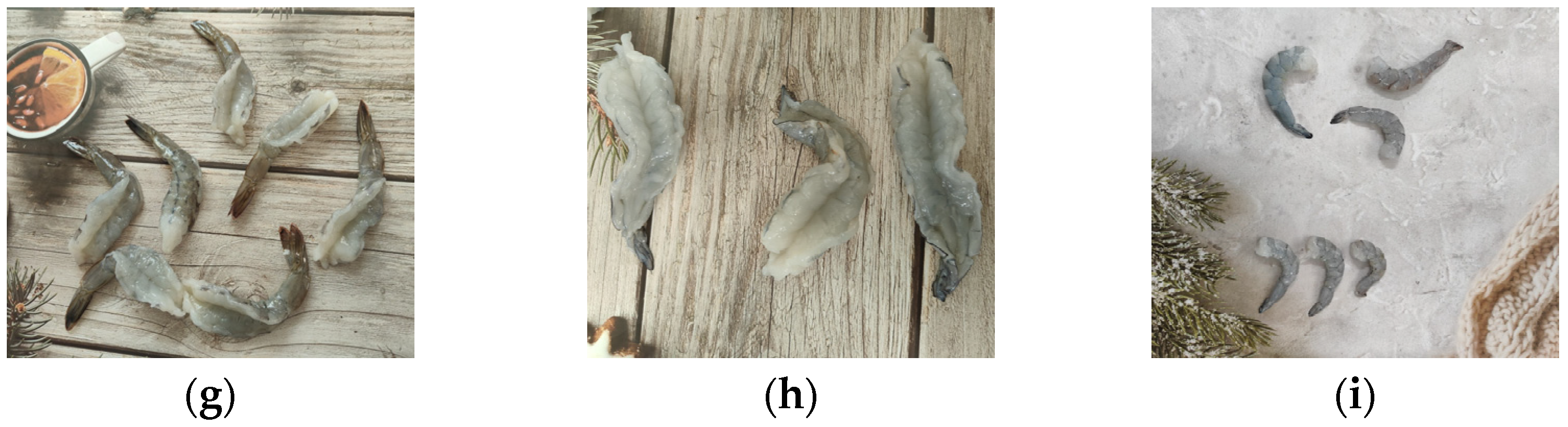
• Quality-defect category: This category included samples exhibiting dehydration and discoloration, damage, incomplete shell removal, incomplete intestinal gland removal, or the presence of shell fragments or appendages (Figure 2a–e), totaling five subcategories;
• Primary processed products: This category comprised fu rong shrimp balls, butterfly shrimp, and butterfly shrimp meat (Figure 2f–h), totaling three subcategories;
• Fully peeled category: This category of shrimp meat has the shell completely removed, and was further subdivided by size into small, medium, and large types (Figure 2i), totaling three subcategories.

To capture a diverse range of shrimp meat images, we utilized both an industrial vision acquisition system and a OnePlus Ace2 smartphone (OPPO, Shenzhen, China). In total, we collected 6186 images, with 4900 images (79.2%) captured by the industrial vision system and 1286 images (20.8%) taken with the OnePlus smartphone. The industrial camera HT-SUA133GC-T (Shenzhen Huateng Vision Technology Co., Ltd., Shenzhen, China), with a resolution of 1280 × 1024 and a 6–60 mm zoom lens, was rigidly positioned approximately 51 cm directly above the sample. Its field of view comprehensively covered the entire white homogeneous background plate, as illustrated in Figure 3. The lighting setup featured a vertical LED panel light with a consistent brightness of 5500 lx. This brightness was dynamically regulated by a specialized controller to replicate a stable shooting environment akin to that of an assembly line conveyor belt, ensuring uniform positioning and illumination. The OnePlus smartphone was furnished with a 16-megapixel front camera and a rear triple-camera system comprising 50 MP + 8 MP + 2 MP lenses. Image capture with the smartphone occurred in two distinct settings: under indoor LED white light (4000 K) and handheld in natural light at a consistent distance. Images taken with the smartphone were evenly distributed among the training, validation, and test datasets, maintaining a proportion of approximately 20%. This allocation aimed to enable the model to accommodate variations in image characteristics arising from diverse acquisition devices.

Following the completion of data collection, a focused data augmentation approach was applied to mitigate category imbalance before data labeling and dataset partitioning. Specifically, categories with limited sample sizes (category 1: 129 original images; category 2: 133 original images; category 3: 130 original images) underwent data augmentation at a 1:10 ratio, resulting in the generation of 10 augmented images for each original image. The augmentation methods employed comprised scaling, horizontal and vertical flipping, random rotation, brightness adjustment, panning, pretzel noise injection, and random masking. These techniques were combined randomly to enhance data diversity effectively.

Following the completion of data augmentation, all images (including both original and augmented ones) were subjected to a systematic labeling process to prepare the dataset for model training. The first author of this study conducted image labeling independently using the labelImg 1.8.6 software (open-source, https://github.com/tzutalin/labelImg, accessed on 5 May 2025). Prior to labeling, a comprehensive guideline was established, drawing from food industry standards and expert advice. This guideline precisely outlined the visual characteristics and criteria for bounding box labeling for each shrimp type. To uphold annotation quality and consistency, a rigorous three-stage labeling and validation approach was employed:

• Systematic initial labeling was first performed on all 6186 original images;
• A comprehensive review was conducted, focusing on refining samples with intricate visual characteristics or unclear boundaries.
• A stratified random sampling approach was employed to verify the accuracy of category labels and bounding boxes by sampling the labeling results of all categories at a 10% sampling ratio.

Throughout the sampling procedure, any identified systematic deviations were thoroughly reviewed, leading to the meticulous relabeling of all samples within the pertinent categories. This meticulous process was undertaken to uphold the quality and dependability of the annotated data.

Finally, we divided the 9720 images and corresponding YOLO format labels into datasets. Using a simple random division method, the dataset was divided into training, validation, and test sets in an 8:1:1 ratio, containing 7776 training images, 972 validation images, and 972 test images.

2.3. YOLOv11 Network Structure

YOLOv11, officially released by Ultralytics on 30 September 2024, represents the latest iteration in the YOLO series, further advancing real-time object detection capabilities. Since YOLOv8 [19], the YOLO series has continued to evolve, with YOLOv9 [20] introducing programmable gradient information (PGI) and an improved Adown module for enhanced multi-scale feature representation, while YOLOv10 [21] proposed a real-time end-to-end detection architecture optimizing inference speed and deployment efficiency. Building upon these advances, YOLOv11 features an architecture structured based on four primary components: input, backbone, neck, and head.

The input component manages the initial preprocessing and data augmentation of input images. These steps are crucial for enhancing the model’s robustness against variations in input data and improving its generalization capability to unseen images.

The backbone, based on the CSPDarknet53 [22] architecture, functions as the primary feature extractor. It processes the input image to generate feature maps at multiple scales using several key modules:

• The Conv module utilized stride-2 convolution for efficient downsampling and initial feature extraction.
• The C3K2 module extends the traditional C2f module by incorporating variable kernel sizes and channel separation strategies, thereby enhancing feature representation capacity.
• The SPPF (spatial pyramid pooling fast) module provides an optimized version of traditional SPP, efficiently capturing contextual information at multiple scales with reduced computational cost.
• The C2PSA module integrates the cross-stage partial (CSP) architecture with the polarized self-attention (PSA) mechanism, enhancing the network’s capacity to perceive features across different scales.

The neck component connects the backbone to the head, drawing inspiration from both the feature pyramid network (FPN) [23] and path aggregation network (PAN) [24]. It implements both top-down and bottom-up pathways for feature fusion. This bidirectional feature fusion effectively integrates low-level, high-resolution features with high-level semantic features, thereby improving detection performance for objects of various sizes.

Finally, the head component is responsible for generating the final detection outputs (bounding boxes and class probabilities). A notable enhancement in YOLOv11 compared to YOLOv8 is the implementation of depthwise separable convolution (DSC) within the head, specifically replacing standard convolutions in the classification branch. DSC factorizes a standard convolution into two separate operations: a depthwise convolution (operating on each channel independently) and a pointwise convolution (a 1 × 1 convolution combining the channel outputs). This factorization significantly reduces the parameter count and computational load while preserving the model’s capacity to learn channel-specific features, thereby facilitating faster inference speeds without compromising detection accuracy. In the following section, we elaborate on the enhanced ADL-YOLO target detection model derived from YOLOv11.

3. Methods

3.1. Improved Network Architecture of ADL-YOLO

This section delineates the structural configuration of the ADL-YOLO object detection model within the YOLOv11 framework, tailored for shrimp quality assessment. The model comprises key technical elements: an enhanced downsampling module, a specialized feature extraction and fusion module, and a streamlined multi-scale feature extraction detection head. Figure 4 illustrates the comprehensive design of ADL-YOLO. Subsequent sections elaborate on the specific structural parameters and implementation strategies for each component sequentially.

3.1.1. Adown Module

The conventional downsampling convolutional layer in the YOLOv11 network architecture was substituted with the Adown module [20] to decrease feature map resolution. Figure 5 illustrates a comparison between the conventional downsampling approach (Figure 5a) and the structure of the Adown module (Figure 5b). The configuration and data flow of the Adown module are delineated as follows.

• Input processing involves passing the input feature graph $X$ through an average pooling layer (AvgPool2d) with a 3 × 3 pooling kernel, a step size of 2, and a padding of 1. This operation computes the average of pixel values in each window to generate a smoothed feature map.
• Channel separation involves dividing the average pooled feature map into two parallel branches based on the channel dimension. If the input feature map has $C$ channels, each branch will have ${\displaystyle \frac{C}{2}}$ channels.
• The initial branch processing involves a convolutional layer with a stride of 2 and a 3 × 3 kernel size, facilitating downsampling of the feature map. This convolutional layer accommodates ${\displaystyle \frac{C}{2}}$ input channels and ${\displaystyle \frac{C}{2}}$ output channels.
• The second branch undergoes the following processing steps: initially, it employs a MaxPool2d layer with a pooling kernel size of 2 × 2 and a stride of 2, selecting the maximum value from each window as the output. Subsequently, the maximally pooled output is passed through a standard convolutional layer with a convolution kernel size of 3 × 3 and a stride of 1, maintaining the channel count at ${\displaystyle \frac{C}{2}}$.
• Feature fusion involves combining feature maps from two branches, each with a size half that of the original input, through concatenation along the channel dimension to create the ultimate output feature map. The output feature map retains the original number of channels, denoted $C$.

The mathematical representation of the Adown module can be expressed as:

$$Y=\mathrm{C}\mathrm{o}\mathrm{n}\mathrm{c}\mathrm{a}\mathrm{t}\left(\mathrm{C}\mathrm{o}\mathrm{n}{\mathrm{v}}_{2\times 2}\left(\mathrm{S}\mathrm{p}\mathrm{l}\mathrm{i}{\mathrm{t}}_1\left(\mathrm{A}\mathrm{v}\mathrm{g}\mathrm{P}\mathrm{o}\mathrm{o}\mathrm{l}\left(X\right)\right)\right),\mathrm{C}\mathrm{o}\mathrm{n}{\mathrm{v}}_{2\times 2}\left(\mathrm{M}\mathrm{a}\mathrm{x}\mathrm{P}\mathrm{o}\mathrm{o}\mathrm{l}\left(\mathrm{S}\mathrm{p}\mathrm{l}\mathrm{i}{\mathrm{t}}_2\left(\mathrm{A}\mathrm{v}\mathrm{g}\mathrm{P}\mathrm{o}\mathrm{o}\mathrm{l}\left(X\right)\right)\right)\right)\right),$$

(1)

where $X$ denotes the input feature map, $Y$ denotes the output feature map, $\mathrm{S}\mathrm{p}\mathrm{l}\mathrm{i}{\mathrm{t}}_1$ and $\mathrm{S}\mathrm{p}\mathrm{l}\mathrm{i}{\mathrm{t}}_2$ denote two channel segmentation components, $\mathrm{C}\mathrm{o}\mathrm{n}{\mathrm{v}}_{2\times 2}$ denotes convolution with a stride of 2, Conv denotes standard convolution, AvgPool denotes average pooling, MaxPool denotes maximum pooling, and Concat denotes channel concatenation.

The following section delineates the structural design and implementation specifics of the DSISConv and MSISConv modules.

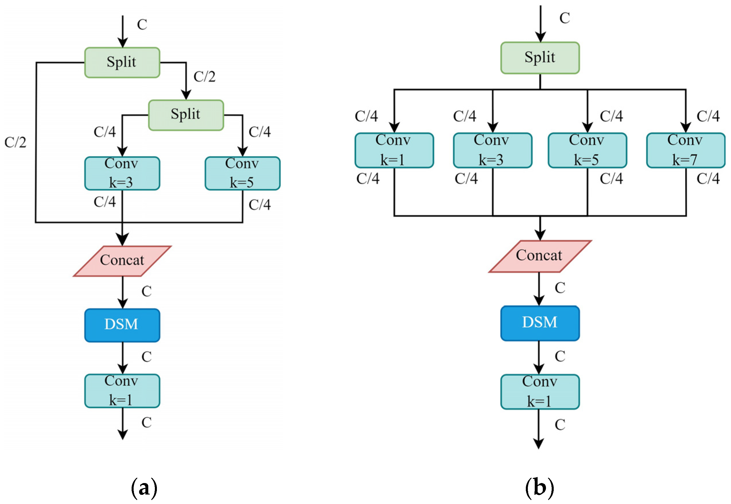
3.1.2. DSISConv and MSISConv Modules

This section presents two novel convolution modules developed for the ADL-YOLO architecture: dual-scale information selection convolution (DSISConv) and multi-scale information selection convolution (MSISConv). These modules were designed to process features at multiple scales while incorporating information selection mechanisms. The following subsections describe the structure and mathematical formulations of these modules, beginning with their foundational components, DSConv and MSConv, followed by the integration of the dual-domain selection mechanism (DSM) to form the complete DSISConv and MSISConv modules.

• Dual-Scale Convolution (DSConv)

The DSConv module combined convolutional kernels of different scales to process the input features. Given an input feature map $X\in {\mathbb{R}}^{N\times C\times H\times W}$, it was first split into two parts along the channel dimension: $X_1\in {\mathbb{R}}^{N\times {\displaystyle \frac{C}{2}}\times H\times W}$ and $X_2\in {\mathbb{R}}^{N\times {\displaystyle \frac{C}{2}}\times H\times W}$. Here, $X_1$ preserve the original feature information, while $X_2$ was further divided into $X_{\mathrm{2,1}}\in {\mathbb{R}}^{N\times {\displaystyle \frac{C}{4}}\times H\times W}$ and $X_{\mathrm{2,2}}\in {\mathbb{R}}^{N\times {\displaystyle \frac{C}{4}}\times H\times W}$, processed by 3 × 3 and 5 × 5 convolutions, respectively, to capture both local and global features across different receptive fields. The outputs of these three branches were then concatenated along the channel dimension and fused via a 1 × 1 convolution, producing the final output $Y\in {\mathbb{R}}^{N\times C\times H\times W}$. The process can be formally expressed as:

$$Y={\mathrm{C}\mathrm{o}\mathrm{n}\mathrm{v}}_{1\times 1}\left(\mathrm{C}\mathrm{o}\mathrm{n}\mathrm{c}\mathrm{a}\mathrm{t}\left(X_1,F_{3\times 3}\left(X_{\mathrm{2,1}}\right),F_{5\times 5}\left(X_{\mathrm{2,2}}\right)\right)\right),$$

(2)

where $\mathrm{C}\mathrm{o}\mathrm{n}\mathrm{c}\mathrm{a}\mathrm{t}$ represents the concatenation operation along the channel dimension and $F_{3\times 3}$ and $F_{5\times 5}$ represent $3\times 3$ and $5\times 5$ convolution operations, respectively.

2.

Multi-Scale Convolution (MSConv)

The MSConv module extends the DSConv design to process input features using four sub-branches. Given an input feature map $X\in {\mathbb{R}}^{N\times C\times H\times W}$, it was first divided into four sub-spaces along the channel dimension. These sub-branches were processed in parallel using convolutional kernels of sizes 1 × 1, 3 × 3, 5 × 5, and 7 × 7 to capture key information from local fine structures to broader receptive fields. The outputs from these four parallel branches were then concatenated along the channel dimension and integrated through a 1 × 1 convolution, producing the final feature map $Y\in {\mathbb{R}}^{N\times C\times H\times W}$. The computation was defined as:

$$Y={\mathrm{C}\mathrm{o}\mathrm{n}\mathrm{v}}_{1\times 1}\left(\mathrm{C}\mathrm{o}\mathrm{n}\mathrm{c}\mathrm{a}\mathrm{t}\left(F_{1\times 1}\left(X_1\right),F_{3\times 3}\left(X_2\right),F_{5\times 5}\left(X_3\right),F_{7\times 7}\left(X_4\right)\right)\right),$$

(3)

where $X_1$, $X_2$, $X_3$, $X_4$ were the four sub-feature maps obtained by equally dividing $X$ along the channel dimension. $F_{1\times 1},F_{3\times 3},F_{5\times 5},F_{7\times 7}$ represent the respective convolution operations.

Following the original designs of DSConv and MSConv, we incorporated the dual-domain selection mechanism (DSM) introduced by Cui et al. [25] to create the DSISConv and MSISConv modules within the DSConv and MSConv frameworks. In the DSISConv module, input features undergo segmentation into biscales for parallel convolution processing, followed by feature integration from the branches. Subsequently, the connected features are subjected to DSM, comprising the spatial selection module (SSM) for spatial feature processing and the frequency selection module (FSM) for signal filtering in the frequency domain. Likewise, the MSISConv module incorporates the DSM structure following multi-scale (1 × 1, 3 × 3, 5 × 5, 7 × 7) convolutional feature fusion. Figure 6 provides a schematic representation of both modules, delineating the placement of DSM components within each structure. The subsequent Section 3.1.3 and Section 3.1.4 describe the integration of DSISConv into the C3K2 module and the reconstruction of the YOLOv11 detection head using MSISConv, respectively.

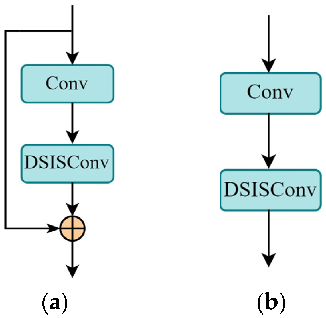
3.1.3. C3K2–DSIS Module

The C3K2–DSIS module was created by integrating the DSISConv module into the C3K2 framework of YOLOv11. This module maintains the fundamental architecture of C3K2, but substitutes the second convolutional layer within the bottleneck structure. Figure 7 depicts the schematic layout of the bottleneck-DSIS block, which functions as the foundational component of C3K2–DSIS. The bottleneck-DSIS block includes a residual connection when its shortcut parameter is set to True (Figure 7a) and omits it when set to False (Figure 7b).

Compared to the traditional C3 module, the C3K module offered the flexibility to select various convolution kernel sizes via configurable parameters, thereby enhancing the diversity and scalability of feature extraction. Building upon this, we replaced the standard bottleneck blocks within the C3K module with our improved bottleneck-DSIS blocks to form the C3K–DSIS module (Figure 8).

Subsequently, the original C3K module was further replaced with C3K–DSIS, yielding the C3K2–DSIS module (Figure 9). When C3K is set to True, the C3K–DSIS serves as the basic building block (Figure 9a), whereas if C3K is set to False, the Bottleneck-DSIS is used instead (Figure 9b).

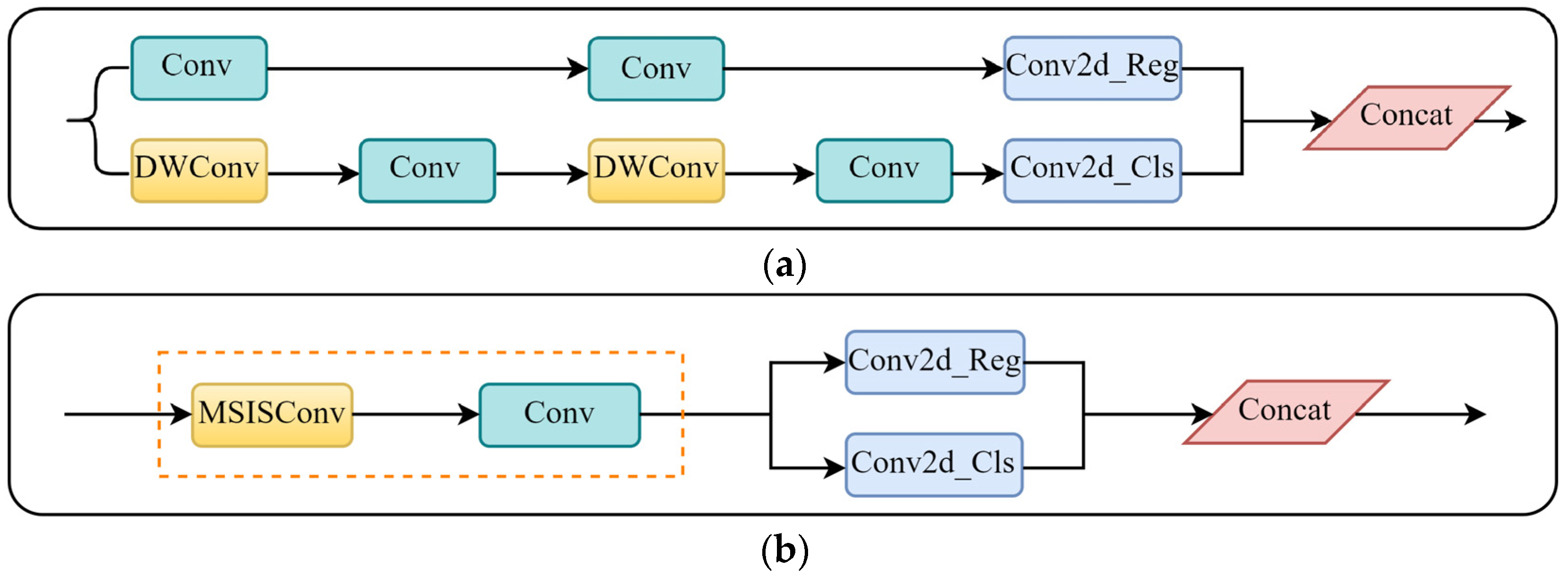
3.1.4. Lightweight Multi-Scale Information Selection Detection Head (LMSISD)

This section delineates the lightweight multiscale information selection detection head (LMSISD), illustrated in Figure 10b. In contrast to the conventional detection head of YOLOv11 (Figure 10a), the LMSISD incorporates the following pivotal design components.

• Parameter sharing in LMSISD, influenced by RetinaTrack, involves sharing parameters across various scale prediction branches (P3, P4, P5). In contrast, the conventional YOLOv11 detector head employs distinct convolutional layers for each scale of feature maps in P3, P4, and P5.
• The MSISConv module was integrated into the detection head structure to process feature maps from three resolutions (80 × 80, 40 × 40, and 20 × 20) before the final prediction layer.
• Decoupled header architecture: LMSISD employs a decoupled framework that segregates the classification and regression tasks into autonomous branches, enabling each branch to independently manage its feature representation.

The data flow in LMSISD involves receiving multi-scale features from the backbone network, processing them using the parameter-sharing MSISConv module, and producing final predictions through distinct classification and regression branches. The next section introduces the bidirectional complementary knowledge distillation technique, which further optimized the model’s performance.

3.2. Bidirectional Complementary Knowledge Distillation

This section outlines a bidirectional complementary knowledge distillation strategy employed to enhance model performance. The approach integrates feature distillation and logic distillation methodologies to establish a dual knowledge transfer mechanism between the teacher model and the student model.

Feature distillation was designed to transfer the structural and semantic knowledge embedded in the intermediate representations of the teacher model to the student model, thereby enhancing the student’s ability to capture spatial features and patterns. Let the feature map of the teacher at layer $i$ be denoted $F_T^i\in {\mathbb{R}}^{C_i\times H_i\times W_i}$ and the corresponding feature map of the student $F_S^i\in {\mathbb{R}}^{C_i\times H_i\times W_i}$. The feature distillation loss was defined as Equation (4):

$${\mathcal{L}}_{\mathrm{f}\mathrm{e}\mathrm{a}\mathrm{t}\mathrm{u}\mathrm{r}\mathrm{e}}=\sum _{i\in \mathcal{I}}{\lambda }_{i}D\left(F_T^i,F_S^i\right),$$

(4)

where $\mathcal{I}$ was the set of layers selected for distillation, ${\lambda }_i$ was the importance weight for layer $i$, and $D\left(\cdot ,\cdot \right)$ represented a chosen distance metric.

Logit distillation aligned the pre-softmax outputs (logits) of the teacher and student models to preserve critical information about decision boundaries and interclass relationships. Denote the logit vectors of the teacher and student $z_T,z_S\in {\mathbb{R}}^{\mathrm{K}},$ The logit distillation loss was expressed as Equation (5):

$${\mathcal{L}}_{logit}=D\left(z_T,z_S\right),$$

(5)

where $\mathrm{K}$ was the number of classes.

The bidirectional complementary knowledge distillation strategy simultaneously transferred intermediate-layer features and output-layer logits from the teacher to the student, allowing the student to acquire richer and complementary knowledge. This approach overcame the limitations of conventional unidirectional distillation. As shown in Figure 11, the framework contained two parallel knowledge transfers: the student model above and the teacher model below were connected through Feature-based distillation and logit-based distillation. In feature-based distillation, the middle representation of multiple layers of the teacher model was projected and aligned with the corresponding layers of the student model. In logit distillation, the output layers of the two models were directly matched. The bidirectional arrows in Figure 11 indicate that in addition to the forward transfer of the teacher’s knowledge, the gradient of the student model was also propagated in the reverse direction, facilitating the joint optimization of the two models. The overall distillation objective was formulated as Equation (6):

$${\mathcal{L}}_{\mathrm{a}\mathrm{l}\mathrm{l}}=\alpha \cdot {\mathcal{L}}_{\mathrm{f}\mathrm{e}\mathrm{a}\mathrm{t}\mathrm{u}\mathrm{r}\mathrm{e}}+\beta \cdot {\mathcal{L}}_{\mathrm{l}\mathrm{o}\mathrm{g}\mathrm{i}\mathrm{c}\mathrm{a}\mathrm{l}}+{\mathcal{L}}_{\mathrm{s}\mathrm{t}\mathrm{u}\mathrm{d}\mathrm{e}\mathrm{n}\mathrm{t}},$$

(6)

where $\alpha$ and $\beta$ were hyperparameters controlling the contributions of feature and logit distillation, respectively.

4. Experimental

4.1. Datasets

This study employed not only the custom shrimp meat dataset but also two additional public datasets: the Potato Detection Dataset [26] from the agricultural domain and PASCAL VOC [27,28] from the general object detection domain.

The Potato Detection Dataset contains 8034 images with corresponding YOLO format labels, with 7188, 576, and 270 images allocated to training, validation, and testing sets respectively. The dataset includes five categories: “damaged potato”, “defected potato”, “diseased-fungal potato”, “potato”, and “sprouted potato”.

The PASCAL VOC dataset consists of 20 common object categories with diverse target size distributions. This study employed the VOC07+12 combination method, which merged the training and validation sets of VOC2007 and VOC2012 for training, while using the VOC2007 test set for validation.

Table 1. Statistics of the images and objects in the VOC07+12 dataset.

Datasets	Train		Val		TrainVal		Test
	Images	Objects	Images	Objects	Images	Objects	Images	Objects
VOC2007	2501	6301	2510	6307	5011	12,608	4952	12,032
VOC2012	5717	13,609	5823	13,841	11,540	27,450	—	—
VOC07+12	16,551	40,058	4952	12,032	—	—	—	—

presents the statistics of images and objects in the VOC07+12 training and validation sets.

4.2. Experimental Environment

The experimental setup consisted of both offline and online platforms. The offline platform was a desktop computer equipped with an Nvidia GeForce RTX 2080 Ti GPU (11 GB memory), primarily used for experiments on the custom dataset. The online platform included two cloud servers, featuring Nvidia A10 and Nvidia GeForce RTX 3090 GPU (both with 24 GB memory), and was utilized for training and testing models on public datasets. All experiments were conducted using the PyTorch 2.2.2 deep learning framework combined with the Python 3.10.14 and CUDA 12.1 programming environments to fully leverage GPU acceleration for training and inference.

During model training, no official pretrained weights were utilized. Instead, a custom yaml configuration file was employed to build the model from scratch. The main training parameters for the datasets are summarized in

Table 2. Key training parameter settings for the datasets.

Hyperparameters	Configuration
	Custom	Potato Detection	VOC07+12
Epochs	200	200	500
Batch	32	32	8
Image Size	640	640	640
Optimizer	SGD	SGD	SGD
lr0	0.01	0.01	0.01
lrf	0.01	0.01	0.01
Close mosaic	0	0	0
Weight decay	0.0005	0.0005	0.0005
Patience	100	100	100
Momentum	0.9	0.9	0.937
Workers	10	10	10
Learning rate decay	Linear decay	Linear decay	Linear decay
Scheduler	LambdaLR	LambdaLR	LambdaLR

.

4.3. Evaluation Metrics

To comprehensively evaluate the detection performance of the proposed model, this study employed the following metrics: precision ($P$), recall ($R$), mean average precision (mAP), frames per second (FPS), model size (Ms), giga floating-point operations (GFLOPs), and parameters (Params). The calculations for precision ($P$) and recall ($R$) are given by Equations (7) and (8):

$$P={\displaystyle \frac{\mathrm{T}\mathrm{P}}{\mathrm{T}\mathrm{P}+\mathrm{F}\mathrm{P}}}$$

(7)

$$R={\displaystyle \frac{\mathrm{T}\mathrm{P}}{\mathrm{T}\mathrm{P}+\mathrm{F}\mathrm{N}}}$$

(8)

where TP represents the number of correctly detected objects and FP and FN denoted the numbers of false positives and false negatives, respectively. Precision ($P$) measured the accuracy of the model’s predictions, while recall ($R$) evaluated the model’s ability to detect targets.

This study followed the standard object detection evaluation protocol, calculating the average precision (AP) under different intersection over union (IoU) thresholds and taking the mean, as shown in Equation (9).

$$\mathrm{m}\mathrm{A}\mathrm{P}={\displaystyle \frac{1}{N}}\sum _{i=1}^N{AP}_i$$

(9)

In this experiment, both mAP50 (mean average precision at an IoU of 0.50) and mAP50-95 (the average of APs across IoUs ranging from 0.50 to 0.95 with a step size of 0.05) were recorded to comprehensively evaluate the model’s performance under different detection precision requirements. Additionally, to accurately reflect the model’s inference speed, the test set was independently evaluated five times. For each test, the time required for preprocessing, inference, and non-maximum suppression (NMS) stages was recorded for each image and averaged. The average FPS was then calculated to ensure the reliability of the evaluation results.

In a multi-metric evaluation system, it was challenging to directly compare indicators with different dimensions to establish a clear ranking of model performance. Therefore, this study adopted the min–max normalization method [29] to scale all performance metrics to the [0, 1] range and assigned corresponding weight coefficients based on the importance of each metric to calculate the comprehensive score for each model. The weighted comprehensive score $W{S}_i$ was calculated as shown in Equation (10).

$$W{S}_i=\sum _{k=1}^8{w}_k\cdot {\displaystyle \frac{M_k-M_{k,\mathrm{m}\mathrm{i}\mathrm{n}}}{M_{k,\mathrm{m}\mathrm{a}\mathrm{x}}-M_{k,\mathrm{m}\mathrm{i}\mathrm{n}}}},$$

(10)

where $w_k$ represented the weight assigned to each performance metric, set as 0.1, 0.1, 0.2, 0.25, 0.2, −0.05, −0.05, and −0.05, respectively. $M_k$ denoted the $\mathrm{k}$-th performance metric, corresponding to $P$, $R$, mAP50, mAP50-95, FPS, Ms, GFLOPs, and Params, while $M_{k,\mathrm{m}\mathrm{i}\mathrm{n}}$ and $M_{k,\mathrm{m}\mathrm{a}\mathrm{x}}$ were the minimum and maximum values of the respective metric across all compared models. The weights were assigned based on the importance of each metric: $P$ and $R$ were assigned weights of 0.1 each to balance precision and recall. mAP50, mAP50-95, and FPS were weighted at 0.2, 0.25, and 0.2, respectively, to emphasize detection accuracy and real-time performance. Ms, GFLOPs, and Params were given weights of −0.05 each to encourage lightweight design and prevent excessive model size and computational complexity.

4.4. Experimental Results and Analysis

The experimental design described in this section followed a hierarchical nesting structure, demonstrating a logical progression. Initially, a multidimensional performance comparison of popular target detection algorithms was conducted on a custom dataset to establish the optimal benchmark model (Section 4.4.1). This benchmark model served as a reliable reference and evaluation standard for subsequent enhancements. Subsequently, the experimental design was structured into three progressive levels to establish a comprehensive optimization verification chain, as follows.

• In the independent evaluation phase assessing the efficacy of enhancement modules (Section 4.4.2 and Section 4.4.3), two fundamental modules underwent scrutiny employing the control variable method within the recognized benchmark model. Firstly, the impact of the ADown downsampling module on reducing model weight was assessed (Section 4.4.2). Secondly, the enhancement in performance of the C3K2–DSIS module in multi-scale feature extraction was validated (Section 4.4.3).
• During the validation phase of module assembly performance (Section 4.4.4 and Section 4.4.5), following the independent evaluation results, the study delved deeper into the benefits of module synergy and integration. The research systematically assessed the collective performance of various downsampling modules when combined with C3K2–DSIS and LMSISD (Section 4.4.4). DSISConv and MSISConv were integrated into the C3K2 structure and lightweight detector head, respectively. This process involved constructing different model variants and conducting a comprehensive comparative analysis to unveil the most effective configuration and its underlying synergy mechanism (Section 4.4.5).
• During the refinement evaluation phase of the ablation experiment (Section 4.4.6 and Section 4.4.7), the efficacy and rationale of each optimization approach were assessed using a refined analysis method. Initially, the optimal embedding position of the module within the network architecture was determined through hierarchical ablation experiments employing C3K2–DSIS (Section 4.4.6). Subsequently, systematic ablation experiments were conducted to quantify the specific impact of each enhanced module on the overall performance, offering a detailed foundation for optimization decisions (Section 4.4.7).

Subsequently, the generalization capacity and applicability of the enhanced model were validated through comparative experiments on publicly available benchmark datasets (Section 4.4.8). Furthermore, a bidirectional complementary knowledge distillation strategy was introduced to enhance the ultimate performance, striking an optimal balance between accuracy and model efficiency (Section 4.4.9).

4.4.1. Performance Comparison of Object Detection Algorithms on the Custom Dataset

This section aimed to systematically evaluate the comprehensive performance of mainstream object detection models in lightweight scenarios, establishing a benchmark for subsequent module optimization. The experiments compared 13 models across three representative algorithmic architectures (anchor-based two-stage algorithms, anchor-based single-stage algorithms, and anchor-free single-stage algorithms) through a unified configuration environment. Evaluation metrics encompassed accuracy ($P$, $R$, mAP), computational efficiency (FPS, GFLOPs), and model scale (parameter count, model size), with weighted synthetic scores ($W{S}_i$) quantifying the trade-off efficiency between models.

Table 3. Performance comparison of mainstream object detection models on the custom dataset.

Model	$\mathit{P}$/%	$\mathit{R}$/%	mAP50 /%	mAP50-95 /%	FPS (Frames/s)	Ms /MB	GFLOPs	Params	$\mathit{W}{\mathit{S}}_{\mathit{i}}$
Anchor-Based One-Stage:
SSD300 [30]	81.9	79.0	85.6	59.6	51.8	212.00	30.926	25,083,000	—
RetinaNet−R50−FPN [31]	72.4	69.3	76.4	52.8	21.6	312.00	179.000	36,537,000	—
YOLOv3−tiny [32]	93.1	91.0	94.6	71.3	271.7	16.60	12.900	8,689,792	0.104
YOLOv5n [33]	94.1	92.8	96.0	74.0	282.5	3.67	4.200	1,774,048	0.486
YOLOv7−tiny [34]	91.8	92.5	95.5	75.3	253.8	11.70	13.100	6,034,656	0.334
Anchor-Free One-Stage:
YOLOv8n [19]	93.1	93.6	96.1	78.9	347.2	5.95	8.100	3,007,793	0.674
YOLOv9t [20]	92.0	93.7	96.5	79.1	207.5	5.82	10.700	2 620 850	0.600
YOLOv10n [21]	93.1	91.8	95.5	78.3	431.0	5.48	8.200	2,698,706	0.583
RT−DETR−R18 [35]	94.6	93.7	95.1	77.2	100.2	38.60	57.000	19,885,884	0.282
YOLOv11n [36]	93.4	94.0	96.1	78.9	328.9	5.21	6.300	2,584,297	0.690
RTMDet−Tiny [37]	91.1	90.8	95.0	76.3	25.7	83.30	8.033	4,876,000	—
YOLOX−tiny [38]	92.6	90.9	95.0	74.1	56.8	65.70	7.579	5,036,000	—
Anchor-Based Two-Stage:
Faster−RCNN −R50−FPN [39]	94.0	92.6	95.9	76.6	19.6	363.00	179.000	41,339,000	—

presents a detailed performance comparison of these detection models across all evaluation dimensions on the custom dataset.

Figure 12 displays the key performance indicators of all lightweight object detection models from Table 3 through radar charts. In Figure 12a, blue-filled areas represented each model’s detection accuracy (mAP50-95, range 70–100%), with each model corresponding to a ray emanating from the center. Correspondingly, Figure 12b has red-filled areas to illustrate the inference speed (FPS, range 0–500) of the same set of models. This radar chart visualization method, through unified coordinate systems and quantification scales, enabled readers to intuitively grasp the trade-off characteristics between accuracy and speed across different architectures, clearly identifying the most advantageous models for specific application scenarios.

Figure 12a demonstrates the accuracy differences among various lightweight object detection models. SSD and RetinaNet performed significantly more poorly than other models, primarily because SSD utilized only a single feature map pyramid structure, where lower-level feature maps, despite having higher resolution, lacked sufficient semantic information, resulting in poor detection of small objects. Although RetinaNet employed feature pyramid networks (FPNs), its heavier ResNet backbone network struggled to fully leverage its advantages in lightweight application scenarios, limiting feature extraction and fusion efficiency. Data from Table 3 further reveal precision differences among YOLO series models. YOLOv9t achieved the highest accuracy among lightweight models, with 79.1% mAP50-95, attributable to its innovative programmable gradient information (PGI) mechanism that preserved complete input information during deep learning processes, effectively avoiding semantic loss problems in traditional deep supervision. YOLOv11n and YOLOv8n (both 78.9%) followed closely, with both models effectively preserving critical feature information while reducing computational redundancy through optimized CSPNet architectures. In contrast, earlier YOLO variants (from YOLOv3-tiny to YOLOv7-tiny) achieved mAP50-95 values of only 71.3–75.3% due to their relatively simple feature extraction networks and limited multi-scale fusion strategies.

Figure 12b visually demonstrates significant differences in inference speed across models. Traditional two-stage detectors such as Faster R-CNN, despite certain accuracy advantages, introduced additional computational steps through region proposal networks (RPNs), significantly increasing inference latency and resulting in the lowest FPS, making them unsuitable for resource-constrained application scenarios. Single-stage detectors like SSD, RetinaNet, and RTMDet simplified the detection process, but remained limited in inference speed due to complex feature extraction backbones and post-processing mechanisms. RTDETR, employing computation-intensive transformer architecture, despite good accuracy, faced similar inference speed constraints. YOLO series, speed-oriented detection frameworks, generally demonstrated higher FPS. Particularly noteworthy was YOLOv10, which completely eliminated traditional non-maximum suppression post-processing steps through innovative NMS-free design, not only simplifying the inference process but also significantly enhancing processing speed, exhibiting the most outstanding speed performance among all comparative models. This design provided an ideal detection solution for real-time application scenarios while maintaining competitive accuracy.

YOLOv5n demonstrated the most outstanding overall scale performance, becoming the lightest detector with only 3.67 MB model size, 4.20 GFLOP computational requirements, and 1.77 M parameters. This was primarily attributed to its coupled head design, which shared feature extraction layers between classification and regression tasks, significantly reducing network complexity. However, this highly parameter-shared design also led to certain losses in feature expression capability, limiting its accuracy performance and exemplifying the trade-off between extreme lightweight design and detection accuracy. YOLOv11n innovatively improved the detection head structure based on YOLOv8n architecture by ingeniously replacing the first convolutional layer of the classification branch with more computationally efficient depth-separable convolutions. This design maintained accuracy levels close to YOLOv8n (78.9% mAP50-95) while reducing parameters to 2.58 M and model size to 5.21 MB, achieving a superior balance between accuracy and scale. The YOLO series, detection framework families focused on lightweight design, generally outperformed other detection architectures in scale control. In comparison, traditional detectors such as SSD and RetinaNet, along with the transformer-based RTDETR, despite outstanding accuracy performance in specific scenarios, significantly increased model scale due to complex feature pyramid structures and large backbone networks, typically requiring over 20 M parameters and exceeding 30 GFLOP computational resources. Particularly prominent were two-stage detectors like Faster R-CNN, where region proposal networks (RPNs) and subsequent classification and regression modules constituted dual computational burdens, exceeding 41 M parameters and 363 MB storage requirements, making deployment difficult in resource-constrained environments.

As evident from Figure 12 and Table 3, modern lightweight detection models generally sought optimal balance points across the three dimensions of accuracy, speed, and model scale. YOLOv9t, YOLOv10, and YOLOv5n represented three design philosophies prioritizing accuracy, speed, and model scale, respectively. YOLOv11n achieved the optimal balance across these three key dimensions with its weighted synthetic index ($W{S}_i=0.690$). Based on YOLOv11n’s optimized balance in network architecture design and computational resource allocation, we selected it as the baseline model, establishing a scientific foundation for subsequent network optimization and application deployment.

4.4.2. Comparison of Detection Performance with Different Downsampling Modules

ADown adopts a dual-branch downsampling structure that parallel-fuses average pooling and max pooling. This section describes the impact on detection performance when integrating ADown and other downsampling modules into the YOLOv11n (baseline) model established in Section 4.4.1. Building on the YOLOv11n (baseline) model’s established performance characteristics, this experiment systematically compared six alternative downsampling implementations while maintaining identical network architectures and training parameters. This controlled-variable approach allowed for direct assessment of each module’s contribution to the detection performance–efficiency trade-off.

Table 4. Performance comparison of different downsampling modules on the custom dataset.

Module	$\mathit{P}$/%	$\mathit{R}$/%	mAP50 /%	mAP50-95 /%	FPS (Frames/s)	Ms /MB	GFLOPs	Params	$\mathit{W}{\mathit{S}}_{\mathit{i}}$
YOLOv11n (Baseline)	93.4	94.0	96.1	78.9	328.9	5.21	6.3	2,584,297	0.566
Context Guided [40]	93.6	93.7	96.9	79.6	282.5	7.07	8.9	3,528,873	0.632
HWD [41]	93.8	94.1	96.7	79.0	306.7	4.52	5.5	2,215,657	0.675
LDConv [42]	91.6	91.7	95.6	77.7	246.3	4.43	5.5	2,170,247	0.047
SPDConv [43]	94.0	93.2	96.7	79.5	303.0	9.01	10.6	4,574,953	0.565
SRFD [43]	93.6	94.2	96.5	79.0	217.4	5.21	7.6	2,555,977	0.445
ADown [20]	92.8	94.4	96.6	79.4	310.6	4.31	5.3	2,105,065	0.695

presents comprehensive performance metrics for each configuration evaluated on the custom dataset.

Comprehensive analysis of Table 4 data revealed ADown to be the optimal downsampling module, demonstrating a 12.9% improvement in weighted comprehensive score (0.695) compared to the YOLOv11n (baseline) configuration (0.566). This superior performance stemmed from ADown’s innovative dual-branch architecture that combined average pooling and max pooling operations. Average pooling preserved global contextual information, while max pooling retained fine-grained edge and texture details, thereby created complementary feature representations. This architectural advantage enabled ADown to maintain competitive accuracy (mAP50 = 96.6%, mAP50-95 = 79.4%) while substantially reduced model parameters by 18.5% and computational cost by 15.9% compared to the YOLOv11n (baseline).

In contrast, modules such as context-guided and HWD demonstrated more balanced accuracy–speed trade-offs through different underlying mechanisms. Context-guided improved accuracy through enhanced receptive field management, but increased model size by 35.7%, thereby limited its efficiency advantages. HWD achieved performance gains through height–width decoupled convolution and effectively reduced parameters while maintained accuracy, resulting in the second-highest comprehensive score (0.675). The notably poor performance of LDConv ($W{S}_i=0.047$) could be attributed to the limited representational capacity of its linear depthwise design when handled the complex features required for precise object detection in our custom dataset. These findings highlighted the critical importance of downsampling module architecture in balancing feature preservation and computational efficiency.

4.4.3. Comparison of Detection Performance with Improved C3K2 Modules

C3K2–DSIS is an enhanced feature extraction module that integrates dual-scale information selection convolution (DSISConv) into the C3K2 architecture. This section describes the effectiveness of our proposed C3K2–DSIS module in comparison with six alternative C3K2 improvements within the detection framework. Building upon the YOLOv11n (baseline) model established in Section 4.4.1 and complementing the downsampling evaluation conducted in Section 4.4.2, this experiment specifically targeted the critical feature extraction backbone component. Through systematic comparison of various C3K2 modifications while maintaining identical network architectures, we isolated each module’s impact on feature representation capacity and computational efficiency. All variants were evaluated under strictly controlled experimental conditions to ensure objective comparison.

Table 5. Performance comparison of different C3K2 modules on the custom dataset.

Module	$\mathit{P}$/%	$\mathit{R}$/%	mAP50 /%	mAP50-95 /%	FPS (Frames/s)	Ms /MB	GFLOPs	Params	$\mathit{W}{\mathit{S}}_{\mathit{i}}$
YOLOv11n (Baseline)	93.4	94.0	96.1	78.9	328.9	5.21	6.3	2,584,297	0.629
C3k2–Faster [44]	92.2	91.7	95.8	78.2	324.7	4.65	5.8	2,290,145	0.579
C3k2–Faster–EMA [44,45]	91.9	92.2	95.7	77.1	274.7	4.70	5.9	2,294,929	0.372
C3k2–gConv [46]	89.8	90.5	94.9	76.2	325.0	4.59	5.7	2,251,809	0.295
C3k2–iRMB [47]	92.8	92.5	95.8	76.8	297.6	4.95	6.0	2,437,201	0.392
C3k2–MogaBlock [48]	89.5	89.3	94.4	75.7	241.5	5.30	6.7	2,570,120	−0.148
C3k2–SCcConv [49]	93.7	93.4	96.4	79.1	310.6	5.00	6.2	2,467,049	0.660
C3K2–DSIS	94.0	94.3	96.8	78.9	331.1	5.14	6.3	2,511,285	0.728

presents comprehensive performance metrics for each module configuration evaluated.

The comparative analysis revealed C3K2–DSIS to be the optimal module, demonstrating a 9.9% improvement in weighted comprehensive score (0.728) compared to the YOLOv11n (baseline) configuration (0.629). This performance improvement derived from C3K2–DSIS’s dual-scale information selection mechanism, which effectively captured both fine-grained and contextual features across multiple spatial dimensions. Notably, C3K2–DSIS improved precision and recall by 0.6% and 0.3%, respectively, while maintaining inference speed (331.1 FPS compared to 328.9 FPS YOLOv11n (baseline)), demonstrated its computational efficiency despite enhanced feature representation.

C3K2–SCcConv demonstrated promising results ($W{S}_i=0.660$) through its spatial channel correlation design, but failed to achieve C3K2–DSIS’s optimal balance of accuracy and efficiency. The underperformance of other variants—particularly C3K2–gConv and C3K2–MogaBlock, exhibiting 1.2–1.7% accuracy decreases—suggested that their architectural innovations, while effective in other domains, created representation bottlenecks within our detection context. C3K2–Faster’s and C3K2–Faster–EMA’s moderate performance indicated their speed optimizations came at the expense of feature quality. These results confirmed that effective multi-scale feature extraction remained crucial for accurate object detection in resource-constrained scenarios.

4.4.4. Performance Comparison of Different Downsampling Modules Combined with C3K2–DSIS and LMSISD

LMSISD (lightweight multi-scale information selection detection head) is a detection framework that integrates multi-scale information selection convolution (MSISConv), adaptively enhancing detection performance across varied object scales. Through its parameter-sharing architecture and decoupled classification and regression branches, LMSISD efficiently captures scale-specific features while maintaining computational efficiency. This section examines the synergistic effects of integrating different downsampling modules with the previously validated C3K2–DSIS (Module B) and LMSISD (Module C) architectural improvements. Building upon the individual module evaluations presented in Section 4.4.2 and Section 4.4.3, this experiment investigated whether these optimal components maintained their efficacy when integrated into a unified architectural framework. By systematically evaluating each downsampling variant in conjunction with fixed B and C modules, the experimental protocol isolated the specific contribution of downsampling design within the enhanced framework while maintaining consistent training parameters across all experimental configurations.

Table 6. Performance comparison of different downsampling modules combined with C3K2–DSIS and LMSISD on the custom dataset.

Module	$\mathit{P}$/%	$\mathit{R}$/%	mAP50 /%	mAP50-95 /%	FPS (Frames/s)	Ms /MB	GFLOPs	Params	$\mathit{W}{\mathit{S}}_{\mathit{i}}$
YOLOv11n (Baseline)	93.4	94.0	96.1	78.9	328.9	5.21	6.3	2,584,297	0.536
+Context Guided + B + C	93.9	93.5	96.6	79.2	238.0	7.55	8.5	3,723,630	0.412
+HWD + B + C	94.6	93.3	96.5	79.3	267.4	5.00	5.1	2,410,414	0.559
+LDConv + B + C	91.4	91.4	95.3	77.6	225.2	4.91	5.1	2,365,004	0.025
+SPDConv + B + C	93.0	93.7	96.8	79.3	278.0	9.49	10.2	4,769,710	0.431
+SRFD + B + C	93.1	94.3	96.4	79.5	207.0	5.69	7.2	2,750,734	0.413
+ADown + B + C	94.3	95.0	96.9	80.2	299.4	4.79	4.9	2,299,822	0.792

presents the comprehensive quantitative performance metrics of these module combinations evaluated on the custom dataset.

The experimental results definitively demonstrated that the ADown + B + C configuration significantly outperformed all alternative combinations, achieving the highest weighted comprehensive score (0.792), representing a substantial 47.8% improvement over the YOLOv11n (baseline) configuration (0.536). This superior performance could be attributed to the inherent architectural complementarity among these modules: specifically, ADown’s dual-branch pooling structure effectively preserved multi-scale features while simultaneously reduced computational demands, thereby established an optimal foundation for C3K2–DSIS’s dual-scale information selection mechanism. Collectively, these architectural components synergistically enhanced LMSISD’s detection capabilities through the provision of optimized multi-scale feature representations.

The proposed architectural combination maintained excellent detection accuracy (mAP50-95 of 80.2%, representing a 1.3% improvement over YOLOv11n (baseline)) while concurrently achieving substantial reductions in computational requirements (22.2% reduction in GFLOPs and 11.0% decrease in parameter count). Although a marginal decrease in inference speed to 299.4 FPS (compared to YOLOv11n (baseline)’s 328.9 FPS) was observed, this 9% reduction was relatively insignificant when contextualized within the framework of the substantial gains achieved in both accuracy and computational efficiency. In contrast, alternative module combinations exhibited less favorable performance trade-offs: specifically, the context-guided + B + C configuration demonstrated comparable accuracy improvements, but necessitated a 45.1% increase in model size and incurred a 27.7% degradation in inference speed, whereas the LDConv + B + C configuration exhibited substantial accuracy deterioration (1.3% decrease in mAP50-95) despite achieving similar reductions in model parameters. These differential experimental outcomes empirically demonstrated that architectural compatibility among integrated modules critically influenced aggregate system performance in ways that transcended their individual modular contributions.

4.4.5. Performance Comparison of Model Variants Based on DSISConv and MSISConv

This section investigates the specific roles and optimal placement of the DSISConv and MSISConv modules within the network architecture. Building on our results from previous experiments (Section 4.4.1, Section 4.4.2, Section 4.4.3 and Section 4.4.4) that demonstrated the effectiveness of each module individually, this experiment examined how these modules interacted when placed at different locations in the network. We designed three variant models—AMD-YOLO, AMM-YOLO, and ADD-YOLO—that systematically alternated the positions of DSISConv and MSISConv within the bottleneck-DSIS and LMSISD components. This experimental design isolated the effect of each module’s placement while preserving the ADown downsampling enhancement, enabling us to identify the configuration that best balanced feature extraction capability and computational efficiency.

Table 7. Performance comparison of variant models and ADL-YOLO on the custom dataset.

Module	$\mathit{P}$/%	$\mathit{R}$/%	mAP50 /%	mAP50-95 /%	FPS (Frames/s)	Ms /MB	GFLOPs	Params	$\mathit{W}{\mathit{S}}_{\mathit{i}}$
YOLOv11n (Baseline)	93.4	94.0	96.1	78.9	328.9	5.21	6.3	2,584,297	0.050
AMD-YOLO	93.4	94.2	97.0	79.7	275.0	4.38	4.4	2,082,126	0.343
ADL-YOLO	94.3	95.0	96.9	80.2	299.4	4.79	4.9	2,299,822	0.610
ADD-YOLO	93.7	94.7	96.9	79.5	287.4	4.27	4.4	2,030,798	0.416
AMM-YOLO	94.6	94.7	97.1	79.7	281.0	4.91	4.9	2,351,150	0.470

provides a comprehensive performance comparison of these variants against YOLOv11n (baseline) and our proposed ADL-YOLO.

As shown in Table 7, ADL-YOLO achieved the highest weighted score ($W{S}_i=0.610$), outperforming all variants despite YOLOv11n (baseline)’s faster inference speed. This superiority was due to ADL-YOLO’s strategic module placement: DSISConv in the bottleneck-DSIS module effectively captured dual-scale features in the backbone, while MSISConv in the LMSISD module enhanced detection precision in the head. Among the variants, AMM-YOLO almost matched ADL-YOLO in accuracy (mAP50 = 97.1%, the highest among all models), but its $W{S}_i$ (0.470) was 22.9% lower due to its less optimal speed–accuracy trade-off.

This pattern revealed a key architectural insight: DSISConv was most effective in the backbone, where dual-scale feature extraction was critical, whereas MSISConv excelled in the detection head, where multi-scale integration was essential for precise localization. This complementarity explained why AMD-YOLO—which reversed these placements—recorded the second-lowest $W{S}_i$ (0.343) despite maintaining reasonable accuracy. ADD-YOLO’s intermediate performance ($W{S}_i=0.416$) further confirmed that although DSISConv benefited the backbone, it lacked the multi-scale integration capabilities required in the detection head. Overall, these results demonstrated that beyond individual module efficacy, the strategic placement of specialized convolution operations within the network significantly influenced detection efficiency.

4.4.6. Hierarchical Ablation Study of C3K2–DSIS

This section examines the optimal placement of C3K2–DSIS modules within the network architecture to maximize performance improvements. Based on the promising results reported in Section 4.4.3 and Section 4.4.5, which demonstrated C3K2–DSIS’s strong feature extraction capabilities, this experiment aimed to identify the specific network layers that benefited most from integrating this module. Instead of applying C3K2–DSIS universally, this study employed a systematic, layer-by-layer ablation methodology to generate eight distinct configurations, each strategically replacing standard C3K2 modules at different network depths. This hierarchical approach yielded fine-grained insights into the architectural impact of feature enhancement modules that standard ablation studies could not provide.

Table 8. Performance comparison of replacing C3K2 modules with C3K2–DSIS at different layers.

Replace Layer	$\mathit{P}$/%	$\mathit{R}$/%	mAP50 /%	mAP50-95 /%	FPS (Frames/s)	Ms /MB	GFLOPs	Params	$\mathit{W}{\mathit{S}}_{\mathit{i}}$
2, 4, 6, 8, 13, 16, 19, 22	95.1	93.9	97.0	79.8	257.73	4.85	4.7	2,266,719	0.307
4, 6, 8, 13, 16, 19, 22	93.0	94.6	96.9	79.7	259.07	4.83	4.7	2,266,864	0.203
6, 8, 13, 16, 19, 22	94.4	94.9	97.1	80.0	270.27	4.82	4.8	2,268,949	0.537
8, 16, 19, 22	94.7	94.5	97.0	80.0	271.74	4.80	4.8	2,286,444	0.477
8, 19, 22	93.8	94.7	96.7	79.5	279.33	4.79	4.9	2,288,529	0.140
8, 19	93.5	95.1	97.0	80.2	292.40	4.82	4.9	2,325,035	0.565
19, 22	93.9	94.7	96.8	80.1	290.70	4.82	4.9	2,325,035	0.407
8, 22	94.3	95.0	96.9	80.2	299.4	4.79	4.9	2,299,822	0.625

summarizes the performance metrics for each configuration evaluated on the custom dataset.

The hierarchical ablation results indicated that selectively replacing C3K2 modules with C3K2–DSIS yielded significantly better performance than applying the module universally across all layers. The configuration that replaced only the 8th and 22nd layers achieved the highest weighted score ($W{S}_i=0.625$), outperforming more extensive replacement configurations with absolute improvements ranging from 8.8% to 48.5%. This optimal configuration maintained high detection accuracy (mAP50 = 96.9%, mAP50–95 = 80.2%), preserved inference speed at 299.4 FPS, and limited the model size to 4.79 MB. These performance patterns demonstrated a clear trade-off between feature representation depth and computational efficiency. Configurations with extensive C3K2–DSIS replacements (particularly layers 2–22 and 4–22) exhibited consistently lower FPS (257.73–259.07) despite comparable accuracy, suggesting computational redundancy in feature processing. This behavior could be attributed to C3K2–DSIS’s dual-scale information selection mechanism, which yielded diminishing returns when applied at every layer and created critical representation bottlenecks when omitted. Strategically placing the module at the 8th and 22nd layers enhanced both shallow and deep features without disrupting internal feature propagation pathways. The 8th layer represented a critical point where spatial resolution remained sufficient for fine-grained feature extraction, whereas the 22nd layer, located near the final detection head, leveraged multi-scale information to directly improve classification and localization accuracy. These findings underscored the importance of targeted architectural modifications, rather than universal module replacement, when optimizing detection networks for resource-constrained environments.

4.4.7. Ablation Study of Improved Modules

This experiment aimed to systematically isolate and quantify the individual and synergistic contributions of the three proposed modules (ADown, C3K2–DSIS, and LMSISD) to overall detection performance. Building upon the promising results from previous experiments in Section 4.4.2, Section 4.4.3, Section 4.4.4, Section 4.4.5 and Section 4.4.6, this comprehensive ablation study followed an incremental design approach, starting with the YOLOv11n (baseline) model and progressively incorporating modules in all possible combinations.

Table 9. Ablation study of the improved modules on the custom dataset. “√” indicates that the module in line 1 was added to the YOLOv11n (baseline) network.

ADown	C3K2–DSIS	LMSISD	$\mathit{P}$/%	$\mathit{R}$/%	mAP50 /%	mAP50-95 /%	FPS (Frames/s)	Ms /MB	GFLOPs	Params	$\mathit{W}{\mathit{S}}_{\mathit{i}}$
			93.4	94.0	96.1	78.9	328.9	5.21	6.3	2,584,297	0.116
√			92.8	94.4	96.6	79.4	310.6	4.31	5.3	2,105,065	0.344
	√		94.0	94.3	96.8	78.9	331.1	5.14	6.3	2,511,285	0.369
		√	93.6	93.9	96.8	79.4	290.7	5.77	6.0	2,852,066	0.176
√	√		94.6	94.2	96.7	79.6	318.5	4.24	5.2	2,032,053	0.539
√		√	94.1	94.7	96.9	79.8	294.1	4.86	5.0	2,372,834	0.490
	√	√	94.2	94.3	96.9	79.6	297.6	5.70	5.9	2,779,054	0.354
√	√	√	94.3	95.0	96.9	80.2	299.4	4.79	4.9	2,299,822	0.642

presents the performance metrics for all module combinations under identical training conditions, providing a complete picture of how these architectural innovations interact.

The ablation results revealed distinct performance profiles for each module and significant synergistic effects in specific combinations. C3K2–DSIS demonstrated the most balanced individual contribution, improving detection accuracy (mAP50 by 0.7%, P by 0.6%) while simultaneously reducing model parameters by 2.8%, confirming its effectiveness in enhancing feature representation without computational penalties. ADown showed a different trade-off profile, reducing model size by 17.3% and GFLOPs by 15.9% while maintaining competitive accuracy, illustrating its primary value in network efficiency. LMSISD, when used independently, achieved strong accuracy gains (0.7% in mAP50, 0.5% in mAP50-95), but at the cost of reduced inference speed (11.6% drop in FPS), highlighting its role as a precision-enhancing component.

The most effective two-module combination (ADown + C3K2–DSIS) delivered a 53.6% weighted score improvement over YOLOv11n (baseline), demonstrating architectural complementarity: ADown’s efficient downsampling preserved essential features while reducing computational demands, creating an ideal foundation for C3K2–DSIS’s multi-scale feature enhancement. This explained why this combination outperformed ADown + LMSISD, which showed similar accuracy but lower efficiency. The full three-module integration maximized performance gains across all accuracy metrics (1.0% in P, 0.8% in R, 1.3% in mAP50-95) while still reducing model size by 8.0% and GFLOPs by 22.2%, achieving an optimal accuracy–efficiency balance.

These findings confirmed the hypothesized complementary mechanisms: ADown optimized feature extraction while preserving informational content, C3K2–DSIS enhanced multi-scale representation capabilities, and LMSISD improved detection precision through better feature utilization. The success of their combination validated the design philosophy of targeting different aspects of the detection pipeline simultaneously rather than focusing on isolated performance metrics.

4.4.8. Generalization Validation on Public Datasets

This experiment aimed to validate the generalization capability and practical applicability of our proposed ADL-YOLO model across diverse datasets beyond the custom training environment. While previous experiments (Section 4.4.1, Section 4.4.2, Section 4.4.3, Section 4.4.4, Section 4.4.5, Section 4.4.6 and Section 4.4.7) evaluated module effectiveness and optimal configurations within a controlled custom dataset, this experiment extended the evaluation to standardized public benchmarks: PASCAL VOC07+12 and Potato Detect. This experimental design was uniquely comprehensive, comparing ADL-YOLO against mainstream lightweight YOLO models. This multi-dataset, multi-baseline approach provided robust verification of whether the architectural advantages demonstrated in controlled experiments translated to real-world detection challenges across various object categories and scales.

Table 10. Performance comparison of different models on the public dataset.

Group	Dataset	Model	mAP50/%	mAP50-95/%	GFLOPs	Params
1	VOC07+12	Yolov5n	74.0	46.9	4.2	1,786,225
2		Yolov7-tiny	79.9	55.2	13.2	6,059,010
3		Yolov8n	80.9	60.2	8.1	3,009,548
4		Yolov10n	81.2	61.5	8.3	2,702,216
5		YOLOv11n (Baseline)	81.5	61.3	6.3	2,586,052
6		ADL-YOLO (Ours)	82.1	62.7	4.9	2,303,881
7	Potato Detect	Yolov5n	76.7	55.3	4.1	1,765,930
8		Yolov7-tiny	78.4	57.1	13.1	6,018,420
9		Yolov8n	79.5	60.2	8.1	3,006,623
10		Yolov10n	77.7	58.7	8.2	2,696,366
11		YOLOv11n (Baseline)	79.6	60.3	6.3	2,583,127
12		ADL-YOLO (Ours)	80.9	61.4	4.9	2,297,116

presents the performance comparison results across these diverse model configurations and datasets.

The comparative analysis across public datasets revealed that ADL-YOLO’s architectural advantages successfully generalized beyond the training environment with consistent performance improvements. On the PASCAL VOC07+12 dataset, ADL-YOLO achieved 82.1% mAP50 and 62.7% mAP50-95, outperforming both the YOLOv11n (baseline) (by 0.6% and 1.4%, respectively) and all other lightweight YOLO variants while requiring 22.2% fewer GFLOPs and 10.9% fewer parameters than YOLOv11n (baseline). This superior accuracy–efficiency balance stemmed from ADL-YOLO’s multi-scale feature processing architecture that effectively captured object features at varying scales—a critical advantage on PASCAL VOC with its diverse object categories and size variations.

On the Potato Detect dataset, which represented a specialized agricultural application scenario, ADL-YOLO demonstrated even more pronounced improvements, with 80.9% mAP50 and 61.4% mAP50-95 scores that exceeded the YOLOv11n (baseline) by 1.3% and 1.1%, respectively. This stronger relative performance improvement on a specialized dataset validated the model’s adaptability to domain-specific detection challenges, where the multi-scale feature handling capabilities proved particularly advantageous for capturing objects with less distinctive features and more variable presentation than common objects.

To provide deeper insights into ADL-YOLO’s category-specific performance characteristics, this analysis examined detection accuracy across all 20 object categories in the PASCAL VOC dataset.

Table 11. Performance comparison of ADL-YOLO and YOLOv11n (baseline) across categories on the PASCAL VOC dataset.

Model	mAP50	Aero	Bicycle	Bird	Boat	Bottle	Bus	Car	Cat	Chair	Cow
YOLOv11n (Baseline)	81.5	87.9	90.6	78.3	74.8	68.0	88.3	91.8	90.2	65.1	82.3
ADL-YOLO	82.1	89.8	91.2	80.5	75.2	69.8	86.8	92.0	91.0	64.7	81.5
Model	Table	Dog	Horse	Moto	Person	Plant	Sheep	Sofa	Train	Tv
YOLOv11n (Baseline)	78.4	86.0	91.3	88.1	88.3	53.1	80.5	78.9	89.3	79.3
ADL-YOLO	77.3	87.1	91.6	88.1	88.3	58.2	82.4	78.7	89.7	79.1

presents the AP50 scores for each category, comparing ADL-YOLO against YOLOv11n (baseline). Figure 13 provided a more intuitive visual comparison of these results, making the performance differences between categories more clearly visible.

The category-wise performance analysis revealed distinctive patterns in how ADL-YOLO’s architectural improvements impacted different object categories, with performance gains that correlated strongly with object scale characteristics. For small objects, which traditionally challenge detection systems, ADL-YOLO demonstrated the most substantial improvements: plant (+5.1%), bird (+2.2%), and bottle (+1.8%). This enhanced small-object detection capability stemmed directly from the dual-scale information selection mechanism, which preserved fine-grained features that would otherwise be lost in conventional downsampling operations.

For medium-sized and large objects, ADL-YOLO maintained consistent performance improvements across categories such as sheep (+1.9%), dog (+1.1%), and car (+0.2%). The multi-scale feature fusion strategy effectively balanced local detail preservation with global context integration, enabling more robust boundary delineation for larger objects. Particularly noteworthy was ADL-YOLO’s performance on categories with significant intra-class scale variation, such as person (maintained at 88.3%) and cat (improved from 90.2% to 91.0%), demonstrating the architecture’s adaptive capability to handle objects that appear at varying sizes within the same category.

The performance pattern aligned with theoretical expectations: the dual-branch feature extraction in ADown combined with selective scale-aware processing in C3K2–DSIS produced greatest benefits for categories where fine-grained feature retention was critical. Conversely, the minor performance decreases observed in the bus (−1.5%) and table (−1.1%) categories could be attributed to these objects’ typically consistent large-scale presentation, where the additional computational overhead of multi-scale processing provided minimal advantages over conventional approaches.

As shown in Figure 13, ADL-YOLO’s performance curve exceeded the YOLOv11n (baseline) model across most categories, with improvements particularly evident in small-object categories such as plant. This visual comparison intuitively confirmed the adaptability and robustness of the proposed multi-scale feature fusion strategy when handling targets of different scales.

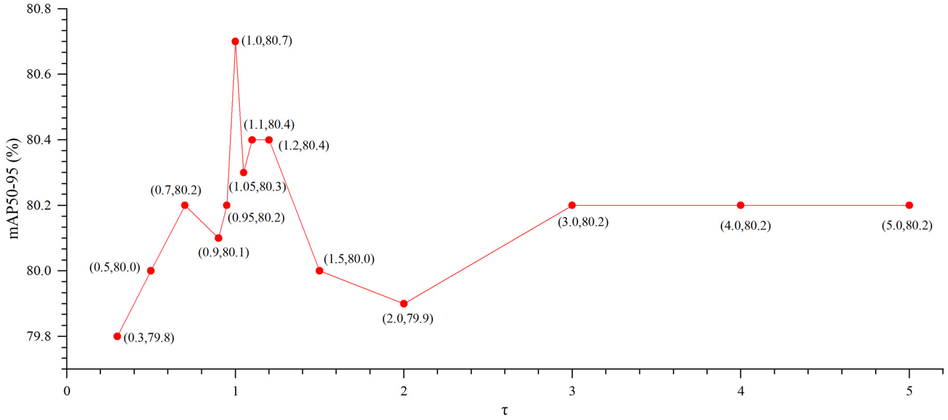
4.4.9. Knowledge Distillation Experiment

This experiment aimed to evaluate the effectiveness of bidirectional complementary knowledge distillation as a final optimization step, building upon the structural improvements validated in Section 4.4.2, Section 4.4.3, Section 4.4.4, Section 4.4.5, Section 4.4.6, Section 4.4.7 and Section 4.4.8. Unlike earlier experiments that optimized network architecture through module design, this experiment focused on enhancing model performance through knowledge transfer without modifying the architectural structure. The experimental design uniquely compared three categories of distillation methods: feature-based methods (Mimic, CWD), logit-based methods (L1, L2, BCKD), and feature–logit combination strategies. By utilizing ADL-YOLO-L as the teacher model and ADL-YOLO as the student model and strategically selecting target layers (the 8th, 13th, 16th, 19th, and 22nd layers), this experiment systematically assessed the impact of different knowledge transfer mechanisms on detection capabilities.

Table 12. Detection performance comparison of different knowledge distillation methods on the custom dataset.

Method	$\mathit{P}$/%	$\mathit{R}$/%	mAP50/%	mAP50-95/%
ADL-YOLO-L (Teacher)	94.3	94.9	97.1	81.4
ADL-YOLO (Student)	94.3	95.0	96.9	80.2
Feature-Based Distillation
Mimic [50]	94.3	94.3	97.1	79.9
CWD [51]	94.4	94.9	96.9	79.9
Logits-Based Distillation
L1 [52]	93.7	94.9	96.7	80.0
L2 [53,54]	94.1	94.9	97.0	80.0
BCKD [55]	94.2	95.8	97.1	80.3
Feature-Logits-Based Distillation
L1 + Mimic	93.6	94.8	96.8	79.9
L1 + CWD	94.5	95.2	97.0	80.4
L2 + Mimic	94.2	94.8	97.0	80.0
L2 + CWD	94.2	95.7	97.1	80.0
BCKD + Mimic	94.1	95.0	97.3	80.4
BCKD + CWD	94.2	96.2	97.4	80.7

presents the performance comparison results of these different distillation strategies on a custom dataset.

The results in Table 12 demonstrate that the BCKD + CWD combination achieved the most significant performance improvement, increasing $R$ by 1.2% and mAP50-95 by 0.5% compared to the student model. This combination even surpassed the teacher model, reaching a recall rate of 96.2% (higher than the teacher model’s 94.9%) and an mAP50 of 97.4% (higher than the teacher model’s 97.1%). This exceptional performance stemmed from the complementarity of the two methods: BCKD’s category alignment mechanism effectively transferred class inference knowledge, while CWD’s channel-level distillation preserved spatial feature relationships crucial for localization.

Single distillation methods exhibited different performance characteristics. Logit-based methods better maintained classification accuracy, with BCKD achieving the same mAP50 (97.1%) as the teacher model. Feature-based methods, while preserving structural consistency, encountered difficulties in feature transformation between models of different capacities, resulting in a 0.3% decrease in mAP50-95 compared to the student model.

Combined methods presented a distinct performance gradient, with BCKD + CWD performing best, followed by BCKD + Mimic, L2 + CWD, and L1 + Mimic, respectively. This progression indicated that the combination of high-level knowledge of class boundaries with spatial relationship information created the most effective knowledge transfer pathway, confirming the importance of multi-level knowledge integration in object detection.

To systematically reveal the synergistic effects of combining BCKD and CWD, we conducted fine-tuning experiments on the key hyperparameters of both methods. By analyzing performance patterns under different parameter configurations, we investigated the intrinsic mechanisms when these two knowledge distillation methods were used in combination. First, we conducted a systematic study on the distillation temperature ($\tau$) in the CWD method. The $\tau$ parameter controls the degree of “softening” in feature distributions and has a decisive impact on channel-level knowledge transfer effectiveness.

Table 13. The effect of distillation temperature ($\tau$) on model performance in the CWD method.

Group	$\mathit{\tau }$	$\mathit{P}$/%	$\mathit{R}$/%	mAP50/%	mAP50-95/%
1	0.3	94.1	94.5	97.0	79.8
2	0.5	94.0	95.5	97.2	80.0
3	0.7	94.1	94.6	97.0	80.2
4	0.9	94.2	95.7	97.4	80.1
5	0.95	94.7	94.5	97.1	80.2
6	1.0	94.2	96.2	97.4	80.7
7	1.05	95.1	95.1	97.4	80.3
8	1.1	94.2	95.5	97.2	80.4
9	1.2	94.6	95.2	97.2	80.4
10	1.5	94.7	94.8	97.2	80.0
11	2.0	94.1	95.7	97.0	79.9
12	3.0	94.8	95.7	97.1	80.2
13	4.0	94.2	94.9	97.2	80.2
14	5.0	94.2	94.9	97.1	80.2

presents the performance trends of the model under different $\tau$ values.

Figure 14 visually illustrates the mAP50-95 trends across all τ values from Table 13 using a line graph.

Data analysis revealed a distinct non-linear relationship between mAP50-95 and $\tau$. When $\tau$ increased from 0.3 to 0.7, performance showed a steady upward trend. Within the interval from $\tau =0.7$ to $\tau =0.95$, performance exhibited slight fluctuations, characterized by a decrease followed by an increase, subsequently reaching the global optimum (mAP50-95 = 80.7%) at $\tau =1.0$. Fine-tuning experiments around the optimal point ($\tau =1.1$, $\tau =1.2$) failed to yield higher performance, further validating the optimality of $\tau =1.0$. As $\tau$ continued to increase to the 1.2–2.0 range, performance displayed a significant downward trend, while in the higher temperature range (2.0–5.0), model performance slightly rebounded before stabilizing, yet consistently remained below the optimal level achieved at $\tau =1.0$.

After determining the optimal distillation temperature $\tau =1.0$, we further optimized the loss weight configuration in the BCKD method. In these experiments, we separately adjusted the classification loss coefficient ${\gamma }_1$ and localization loss coefficient ${\gamma }_2$ to evaluate their marginal contributions and interaction effects on detection performance. The experimental results are summarized in

Table 14. The impact of classification loss coefficient (${\gamma }_1$) and localization loss coefficient (${\gamma }_2$) on detection performance in the BCKD method.

Group	${\mathit{\gamma }}_1$	${\mathit{\gamma }}_2$	$\mathit{P}$/%	$\mathit{R}$/%	mAP50/%	mAP50-95/%
1	1.0	7.5	94.2	96.2	97.4	80.7
2	0.5	7.5	94.0	95.1	97.2	80.2
3	0.1	7.5	94.8	95.1	97.3	80.0
4	2.0	7.5	94.2	95.2	96.8	79.7
5	1.0	7.0	94.3	95.3	97.0	80.2
6	1.0	6.9	93.8	94.6	97.1	80.2
7	1.0	6.8	94.4	94.6	97.2	80.4
8	1.0	6.7	94.6	95.2	97.2	80.3
9	1.0	6.6	95.3	95.0	97.2	80.1
10	1.0	6.4	94.6	94.8	97.2	80.3
11	1.0	6.3	94.4	94.6	97.0	80.1
12	1.0	6.2	94.5	94.9	96.9	80.0
13	1.0	6.1	94.2	95.0	97.2	80.3
14	1.0	6.0	94.0	95.5	97.2	80.4
15	1.0	5.5	94.2	94.3	97.0	80.1
16	1.0	5.0	94.1	95.6	97.0	80.2
17	0.1	6.1	93.5	95.5	97.1	80.3
18	0.1	2.0	93.7	94.7	97.1	80.0
19	0.1	1.0	94.3	95.0	97.1	79.9

.

The data in Table 14 indicate that the initial configuration (${\gamma }_1=1.0$, ${\gamma }_2=7.5$) performed best across key metrics, including $P$, $R$, mAP50, and mAP50-95. Adjustments to ${\gamma }_1$ significantly impacted mAP metrics, with its optimal value remaining stable at 1.0, while ${\gamma }_2$ maintained high performance within the range of 6.0–7.5, with the ${\gamma }_2=6.0$ configuration also achieving near-optimal mAP50-95 (80.4%).

Based on the results of parameter optimization experiments, we can clearly articulate the synergistic working mechanism of the BCKD and CWD combination:

BCKD primarily targets the network output layer, achieving knowledge alignment at the decision level through structured supervision signals, ensuring that the student model accurately replicates the teacher model’s classification judgments and bounding box regression capabilities. CWD, in contrast, focuses on the intermediate feature layers of the network, transferring the teacher model’s internal representation mechanisms by modeling channel weight relationships and spatial attention distributions. This complementary multi-level knowledge transfer establishes a coherent knowledge migration pathway, enabling the student model to comprehensively acquire both the feature representation methods and decision logic of the teacher model.

Hyperparameter tuning experiments demonstrated that BCKD and CWD each achieved their optimal performance under the parameter configuration (${\gamma }_1=1.0$, ${\gamma }_2=7.5$, $\tau =1.0$) and produced significant synergistic effects when used in combination. Under this configuration, BCKD balanced the supervision intensity of classification and regression tasks through appropriate loss weight ratios, while CWD accurately transferred channel-level feature representations through the optimal temperature parameter. Comparative experimental data indicated that deviation of any parameter from its optimal value resulted in performance degradation, confirming the principle of balanced multi-level information transfer in knowledge distillation.

Quantitative analysis in Table 12 reveals that the combined application of BCKD and CWD achieved a consistent improvement of 0.3–0.5 percentage points in the mAP50-95 metric compared to using either method alone. Further verification through controlled variable experiments confirmed that this gain was not a simple additive effect, but stemmed from mutual enhancement between the two methods: the intermediate layer feature representations optimized by CWD provided a high-quality foundation for BCKD, while BCKD’s precise constraints on the output layer provided clearer feature learning signals through the backpropagation mechanism, forming a mutually reinforcing optimization process. This interactive enhancement relationship between feature layers and output layers provides important empirical support and methodological insights for knowledge distillation research in the field of object detection.

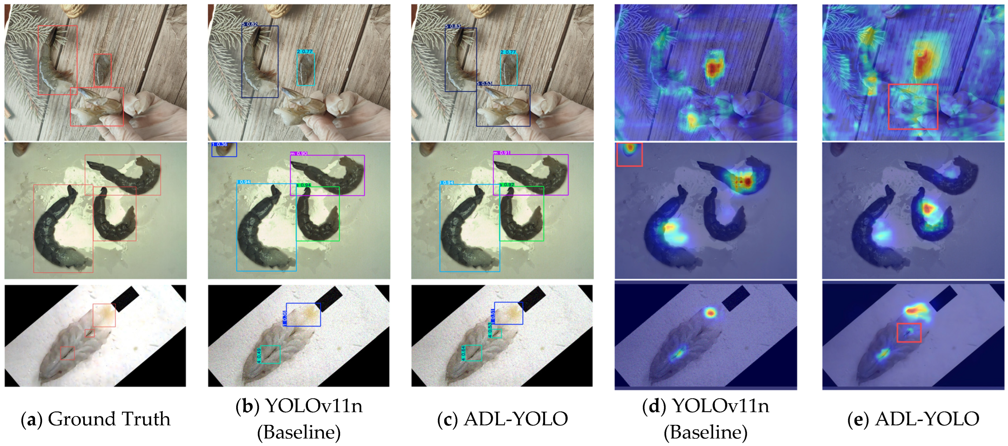
4.5. Visual Analysis of Results

To evaluate the performance improvements of ADL-YOLO, this section analyzes the results from two perspectives: detection visualization and feature heatmaps [56]. Figure 15 presents a comparison of ADL-YOLO and YOLOv11n (baseline) on the custom shrimp meat dataset. The comparisons include the ground truth (a), YOLOv11n (baseline) detection results (b), ADL-YOLO detection results (c), and their corresponding feature heatmaps (d,e). In addition, Figure 16 presents a visualization comparing the feature attention regions before and after model distillation.

On the custom shrimp meat dataset, ADL-YOLO outperformed YOLOv11n (baseline) in both complex and simple-background scenarios for multi-scale detection and defect identification at different scales. When the background exhibited similarity to the target, ADL-YOLO more accurately focused on object edges and details, thereby reducing false positives and missed detections (see the first two rows in Figure 15). It also demonstrated superior stability when handling small-scale shrimp meat intestines and other minor targets (the third row in Figure 15), further enhancing attention at the defect edges after distillation (Figure 16e).

5. Discussion

5.1. Comparison of ADL-YOLO with Existing Detection Methods

Aquatic product quality inspection presents unique challenges, particularly in simultaneously processing targets of different scales (such as microscopic defects and overall morphological features). The ADL-YOLO model proposed in this study has achieved significant results in addressing these challenges. Lee et al. [3] proposed a shape analysis method based on tangent angle distribution analysis (TADA) and tangent angle cross-correlation (TAC), which, although achieving “93.7% detection rate for good shrimp and 94.2% for damaged shrimp” in simple backgrounds, relies on contour extraction and shape analysis, lacking the capability to handle complex scenes. Similarly, Zhang et al. [4] proposed a method combining evolutionary constructed (ECO) features with AdaBoost classifier, achieving a classification accuracy of 95.1%. However, these traditional methods primarily depend on manually designed features, making it difficult to automatically adapt to multi-scale targets and various morphological variations. In contrast, our approach uses smartphone-captured images with complex backgrounds combined with data augmentation methods, significantly enhancing ADL-YOLO’s detection capability in complex scenarios. More importantly, our model demonstrates excellent performance on the PASCAL VOC dataset, particularly improving detection precision for small target categories such as plants, birds, and bottles by 5.1%, 2.2%, and 1.8%, respectively, while also showing notable improvements for medium-sized to large targets like sheep (+1.9%) and dogs (+1.1%).

Among deep learning methods, ShrimpNet by Hu et al. [7] and Deep-ShrimpNet by Liu et al. [8] represent early attempts, achieving accuracies of 95.48% and 97.2%, respectively. However, they exhibit limitations in computational efficiency and real-time processing. Although ShrimpNet features a simple structure, its feature extraction capability is relatively limited, while Deep-ShrimpNet, improved based on AlexNet and considering feature extraction at different scales, has higher modeling time (0.54 h) and resource requirements, making it difficult to deploy efficiently in resource-constrained industrial environments. In contrast, our ADL-YOLO model, through innovative lightweight design, significantly reduces computational requirements while maintaining high accuracy, making it more suitable for practical industrial applications.

In recent advances in multi-scale object detection, the YOLO-SK algorithm proposed by Wang and Hao [13] represents the latest achievement in lightweight models in multi-scale detection tasks. However, YOLO-SK is primarily designed for general scenarios, whereas our ADL-YOLO focuses on the specific domain of aquatic product quality inspection, addressing the multi-scale detection problem of shrimp body defects more precisely through innovative modules such as DSISConv and MSISConv. Although both methods pursue lightweight models, ADL-YOLO achieves a greater reduction in computational cost (22.2% reduction in GFLOPs) while maintaining high precision, demonstrating the value of deep optimization for specific applications.

Within the YOLO series models, our ADL-YOLO demonstrates clear advantages over YOLOv3-tiny [32], YOLOv5n [33], YOLOv7-tiny [34], YOLOv8n [19], YOLOv9t [20], YOLOv10n [21], and YOLOv11n (baseline) in the task of multi-scale shrimp detection, outperforming the aforementioned models. This is primarily attributed to our three innovative modules.

5.2. Working Mechanisms and Synergistic Effect Analysis of Core Modules

This study introduces three innovative modules (ADown, C3K2–DSIS, LMSISD) and a bidirectional knowledge distillation method that work synergistically to enhance detection performance.

The ADown module employs parallel average and max pooling operations to achieve lightweight downsampling while preserving critical features. In ablation experiments, ADown reduces Ms, GFLOPs, and Params by approximately 17.3%, 15.9%, and 18.5%, respectively, compared to the baseline, with only a marginal 0.6% accuracy cost while improving recall and mAP metrics by 0.4–0.5%.

C3K2–DSIS combines the C3K2 structure with dual-scale information selection convolution (DSISConv) to enhance feature selection precision. When integrated with ADown, performance metrics improve by 0.2–1.2% while simultaneously reducing Ms by 18.6%, GFLOPs by 17.5%, and Params by 21.4%. This module effectively compensates for ADown’s limitations in detail capture while providing refined feature maps for subsequent processing.

The LMSISD module features parameter sharing, decoupled detection heads, and multi-scale information selection convolution (MSISConv). When all three modules operate together, precision, recall, and mAP metrics improve by approximately 0.8–1.3%, with overall system reductions of 8.0% in Ms, 22.2% in GFLOPs, and 7.1% in Params. Although LMSISD slightly reduces FPS, the computational resources saved by the previous modules offset this overhead, maintaining approximately 300 FPS for real-time inference.

Our bidirectional complementary knowledge distillation achieves multi-level alignments in both feature and logit layers, providing an additional 0.4–0.8% improvement in mAP50-95. This approach enhances multi-scale feature representation consistency and strengthens decision boundaries.

The complete architecture creates an efficient technical closed loop: ADown delivers balanced high-quality input, followed by C3K2–DSIS performing dynamic multi-scale filtering, then LMSISD executing deep semantic fusion and fine-grained distribution, with knowledge distillation providing additional alignment at both feature and decision levels. This sequential pipeline of “quality input, then dynamic selection, followed by efficient fusion, and finally distillation optimization” enables mutual amplification of advantages and complementation of deficiencies among modules, achieving an optimal balance between accuracy, speed, and model size for shrimp quality inspection tasks.

5.3. Limitations

Despite the significant achievements of this study, several noteworthy limitations remain.

Regarding sample representativeness, although measures were taken to ensure the capture of batch-to-batch variability, all samples were sourced from a single processing facility, limiting the geographic representativeness of the research findings. While Pacific white shrimp (Litopenaeus vannamei) dominates China’s shrimp aquaculture industry (accounting for over 80% of production), variations in cultivation environments, feeding practices, and processing techniques across different regions may affect the universal applicability of the results. Processing technology differences between facilities even within the same region may also lead to variations in product quality characteristics.

Concerning model performance limitations, although ADL-YOLO demonstrates excellent performance in shrimp quality detection, its effectiveness may be compromised under the following conditions: (1) extreme lighting conditions (such as direct strong light or dark environments) that reduce detection accuracy; (2) severe occlusion or high stacking density of targets, which represents a common challenge in actual processing environments; and (3) exclusive use of visible light imaging, potentially limiting application potential in scenarios requiring additional spectral information.

With respect to computational resources and generalization capability, despite our optimizations reducing model size (Ms) by approximately 8.0%, computational complexity (GFLOPs) by 22.2%, and parameter count (Params) by 7.1%, further optimization space remains for deployment on ultralow-power devices. Additionally, the model’s generalization capability requires improvement when processing shrimp species with distributions significantly different from the training data.

5.4. Industrial Application Potential

ADL-YOLO, with its lightweight architecture (2.3 M Params, 4.9 GFLOPs), demonstrates significant application potential on industrial-grade edge computing devices. To comprehensively evaluate the model’s performance advantages in actual deployment environments,

Table 15. Comparison of model scale and inference performance between ADL-YOLO and existing lightweight object detection models.

Model	Params/M	GFLOPs	Ms/MB	Platform	FPS (Frames/s)	References
GVC-YOLO	2.53	6.8	5.4	Jetson Xavier NX	48.0	Zhang et al. [57]
EdgeTrim-YOLO	6.40	11.0	14.9	RK3588 NPU	34.6	Xu et al. [58]
YOLO v5n	1.90	4.5	4.2	RK3588 NPU	59.9	Xu et al. [58]
YOLO v5s	7.20	16.5	15.7	RK3588 NPU	27.9	Xu et al. [58]
YOLO v5m	21.2	49.0	43.0	RK3588 NPU	16.0	Xu et al. [58]
CFIS-YOLO	7.17	—	11.21	SOPHON BM1684X	135.0	Kang et al. [59]
YOLO-YSTs	3.02	8.8	6.5	Raspberry Pi 4B	22.0	Huang et al. [60]
ADL-YOLO (Ours)	2.3	4.9	4.79	NVIDIA GeForce RTX 2080 Ti	299.4	—

provides a comparative analysis of ADL-YOLO against current mainstream lightweight object detection models, examining model scale and inference speed performance across different edge computing platforms, thus providing reference data for the industrial application of intelligent shrimp quality inspection.

When compared to existing lightweight models, ADL-YOLO exhibits superior computational efficiency. Relative to GVC-YOLO [57], our model reduces computational complexity by 27.9% with only a 9.1% decrease in parameters. Against larger models like YOLOv5s and YOLOv5m [58], ADL-YOLO reduces computational complexity by 70.3% and 90.0% respectively, while substantially decreasing model size. These efficiency gains validate our lightweighting approach.

The model shows promising deployment potential on edge computing hardware. With 44.3% lower computational complexity and 23.8% fewer parameters than YOLO-YSTs [60], ADL-YOLO theoretically enables higher frame rates on constrained hardware like Raspberry Pi 4B. Similarly, compared to CFIS-YOLO [59], our model offers greater deployment flexibility with 211.7% fewer parameters and 134.0% smaller model size, while maintaining competitive performance characteristics.

For practical implementation, ADL-YOLO can be integrated into existing shrimp processing lines through multi-camera systems, excelling at detecting subtle defects often missed by traditional methods. Economically, this automated quality control system can significantly reduce defect rates while remaining affordable for small and medium-sized enterprises due to its reduced hardware requirements and operational costs.

5.5. Future Work

Based on the achievements and limitations of this study, we propose several promising directions for future research.

• Multi-regional data validation and model generalization: Expanding the sampling range to multiple processing facilities across China’s major coastal production areas to assess the impact of geographic location and processing technology differences on detection performance, further validating ADL-YOLO’s adaptability and stability across diverse production environments.
• Extension to other aquatic product detection: Applying the ADL-YOLO framework to quality inspection of fish fillets, squid, and other aquatic products with more complex texture and shape characteristics. Through transfer learning and domain adaptation techniques, the model can efficiently adapt to new food categories, expanding its application scope.
• Domain transfer adaptation enhancement: Investigating model performance stability under varying backgrounds, different shrimp species, and camera parameter conditions. Introducing adversarial training and meta-learning techniques to enhance model robustness in changing environments, particularly developing more universally applicable detection models for species variations across different geographic regions.
• Practical deployment and performance verification across diverse edge computing platforms: Implementing system performance evaluation of ADL-YOLO on various edge computing devices, including Jetson series (Xavier NX, Orin Nano), RK3588 NPU, and Raspberry Pi, verifying its inference speed and resource utilization performance in actual hardware environments.

5.6. Artificial Intelligence Technology Application

This research fully leverages artificial intelligence technology, particularly recent advances in deep learning and computer vision. Our ADL-YOLO model is based on deep convolutional neural network architecture, employing advanced feature extraction and fusion techniques. Knowledge distillation methods, an important technology in contemporary AI research, achieve performance improvements in lightweight models through inter-model knowledge transfer. Additionally, during model training, we applied AI techniques such as data augmentation and transfer learning to enhance the model’s generalization capability.

Overall, the success of ADL-YOLO validates the immense potential of artificial intelligence technology in solving practical industrial problems, providing an efficient and accurate technical solution for the food safety and quality control domain.

6. Conclusions

This study presents ADL-YOLO, a lightweight multi-scale object detection model based on YOLOv11n, specifically designed to address the technical challenges of shrimp quality inspection. Through a series of innovative modules, the method significantly improved detection performance while maintaining computational efficiency, providing an important technological breakthrough for automated quality control in the food industry.

We first introduced the ADown module as the core downsampling component of ADL-YOLO. Unlike the stride-2 convolutional downsampling commonly used in object detection networks, the ADown module combined the advantages of average pooling and max pooling, effectively reducing feature map dimensions while maximizing the preservation of original feature information integrity. This dual-path pooling strategy enabled our network to demonstrate stronger robustness when processing targets of different scales. Next, we proposed two innovative convolution structures: dual-scale information selection convolution (DSISConv) and multi-scale information selection convolution (MSISConv). Traditional convolutions use only single-scale kernels for feature extraction, limiting feature representation capabilities. The DSISConv module, based on the CSPNet structure, captured target features from different receptive fields through parallel deployment of dual-scale convolutions, followed by feature fusion. MSISConv went further by simultaneously extracting features using four different dimensional convolution kernels in parallel, concatenating them in the channel dimension to achieve more comprehensive feature representation. These two convolution structures significantly enhanced the network’s perception of multi-scale targets. More crucially, we introduced a dual-domain selection mechanism (DSM) in both modules, which adaptively filtered task-relevant high-quality features, both enhancing feature representation capability and reducing computational redundancy. Furthermore, we designed a lightweight multi-scale information selection detection head (LMSISD), revolutionizing the concept of detection head design. Unlike YOLOv5’s fully coupled design and YOLOv8’s fully decoupled approach, LMSISD innovatively adopted a “couple first, decouple later” strategy: first processing input features through a parameter-sharing mechanism, then extracting and filtering high-quality multi-scale features using MSISConv, and finally decoupling into independent classification and regression branches. This design significantly improved the detection head’s perception of targets at different scales through multi-scale feature fusion while maintaining efficient parameter utilization. The bidirectional complementary knowledge distillation method overcame the limitations of traditional unidirectional distillation. This method achieved synchronous knowledge transfer at both feature and output layers, enabling complementary enhancement of low-level feature representation learning and high-level category discrimination capability, comprehensively improving model performance.

Ablation experiments on the improved modules demonstrated that compared to YOLOv11n (baseline), ADL-YOLO achieved comprehensive performance improvements: precision ($P$) increased by 1.0%, recall ($R$) by 0.8%, mAP50 by 0.9%, and mAP50-95 by 1.3%. Simultaneously, while maintaining a high inference speed of 299.4 FPS, parameter count was reduced by 7.1%, model size by 8.0%, and computational complexity by 22.2%. Cross-validation experiments on public datasets further confirmed the model’s generalization ability: on the VOC07+12 dataset, compared to YOLOv11n (baseline), mAP50 improved by 0.6% and mAP50-95 by 1.4%; on the Potato Detect dataset, mAP50 and mAP50-95 improved by 1.3% and 1.1% respectively, indicating that ADL-YOLO demonstrated robust adaptability across object detection tasks in different domains. Additionally, knowledge distillation experiments further enhanced ADL-YOLO’s performance, improving precision ($P$) by 0.1%, recall ($R$) by 1.2%, and providing additional gains of 0.5% for both mAP50 and mAP50-95. Notably, compared to single distillation methods, our bidirectional complementary knowledge distillation method provided an additional 0.4–0.8% improvement in mAP50-95, further optimizing overall performance.

In conclusion, ADL-YOLO not only achieved synergistic optimization of accuracy and efficiency in the specific scenario of shrimp quality inspection, but its excellent performance on diverse datasets also demonstrated the model’s good cross-domain generalization capability and practical value. Nevertheless, we objectively recognize the current research limitations: first, there remains room for improvement in the diversity of training samples regarding environmental conditions and target distribution; second, model robustness under extreme lighting, temperature, and humidity conditions requires further validation; and finally, although the model has achieved lightweight design, deployment optimization on ultralow-power edge devices still requires more in-depth engineering adaptation. Looking ahead, we plan to expand research in three directions: extending the application domain to broader aquatic products and food quality inspection, developing domain transfer technologies with stronger environmental adaptability, and exploring synergistic optimization of model structure and quantization compression to accommodate resource-constrained industrial terminal devices.

References

1. FAO. The State of World Fisheries and Aquaculture 2024; Food and Agriculture Organization of the United Nations: Rome, Italy, 2024; Available online: https://www.fao.org/documents/card/en/c/cc9840en (accessed on 27 March 2025).
2. Wang, J.; Che, B.; Sun, C. Spatiotemporal variations in shrimp aquaculture in China and their influencing factors. Sustainability 2022, 14, 13981. [Google Scholar] [CrossRef]
3. Lee, D.J.; Xiong, G.M.; Lane, R.M.; Zhang, D. An Efficient Shape Analysis Method for Shrimp Quality Evaluation. In Proceedings of the 2012 12th International Conference on Control Automation Robotics & Vision (ICARCV), Guangzhou, China, 5–7 December 2012; pp. 865–870. [Google Scholar]
4. Zhang, D.; Lillywhite, K.D.; Lee, D.J.; Tippetts, B.J. Automatic shrimp shape grading using evolution constructed features. Comput. Electron. Agric. 2014, 100, 116–122. [Google Scholar] [CrossRef]
5. Liu, Z.; Jia, X.; Xu, X. Study of shrimp recognition methods using smart networks. Comput. Electron. Agric. 2019, 165, 104926. [Google Scholar] [CrossRef]
6. Zhou, C.; Yang, G.; Sun, L.; Wang, S.; Song, W.; Guo, J. Counting, locating, and sizing of shrimp larvae based on density map regression. Aquac. Int. 2024, 32, 3147–3168. [Google Scholar] [CrossRef]
7. Hu, W.; Wu, H.; Zhang, Y.; Zhang, S.; Lo, C. Shrimp recognition using ShrimpNet based on convolutional neural network. J. Ambient. Intell. Humaniz. Comput. 2020, 1–8. [Google Scholar] [CrossRef]
8. Liu, Z.H. Soft-shell Shrimp Recognition Based on an Improved AlexNet for Quality Evaluations. J. Food Eng. 2020, 266, 109698. [Google Scholar] [CrossRef]
9. Tian, Y.; Wang, S.; Li, E.; Yang, G.; Liang, Z.; Tan, M. MD-YOLO: Multi-scale Dense YOLO for small target pest detection. Comput. Electron. Agric. 2023, 213, 108233. [Google Scholar] [CrossRef]
10. Tao, H.; Zheng, Y.; Wang, Y.; Qiu, J.; Stojanovic, V. Enhanced feature extraction YOLO industrial small object detection algorithm based on receptive-field attention and multi-scale features. Meas. Sci. Technol. 2024, 35, 105023. [Google Scholar] [CrossRef]
11. Li, Y.-L.; Feng, Y.; Zhou, M.-L.; Xiong, X.-C.; Wang, Y.-H.; Qiang, B.-H. DMA-YOLO: Multi-scale object detection method with attention mechanism for aerial images. Vis. Comput. 2023, 40, 4505–4518. [Google Scholar] [CrossRef]
12. Cao, Y.; Li, C.; Peng, Y.; Ru, H. MCS-YOLO: A Multiscale Object Detection Method for Autonomous Driving Road Environment Recognition. IEEE Access 2023, 11, 22342–22354. [Google Scholar] [CrossRef]
13. Wang, S.; Hao, X. YOLO-SK: A lightweight multiscale object detection algorithm. Heliyon 2024, 10, e24143. [Google Scholar] [CrossRef] [PubMed]
14. Wang, L.; Liu, X.; Ma, J.; Su, W.; Li, H. Real-Time Steel Surface Defect Detection with Improved Multi-Scale YOLO-v5. Processes 2023, 11, 1357. [Google Scholar] [CrossRef]
15. Guo, Y.; Chen, S.; Zhan, R.; Wang, W.; Zhang, J. LMSD-YOLO: A Lightweight YOLO Algorithm for Multi-Scale SAR Ship Detection. Remote. Sens. 2022, 14, 4801. [Google Scholar] [CrossRef]
16. Peng, S.; Fan, X.; Tian, S.; Yu, L. Ps-yolo: A small object detector based on efficient convolution and multi-scale feature fusion. Multimed. Syst. 2024, 30, 241. [Google Scholar] [CrossRef]
17. Su, Z.; Yu, J.; Tan, H.; Wan, X.; Qi, K. MSA-YOLO: A Remote Sensing Object Detection Model Based on Multi-Scale Strip Attention. Sensors 2023, 23, 6811. [Google Scholar] [CrossRef]
18. Li, J.; Sun, H.; Zhang, Z. A Multi-Scale-Enhanced YOLO-V5 Model for Detecting Small Objects in Remote Sensing Image Information. Sensors 2024, 24, 4347. [Google Scholar] [CrossRef]
19. Glenn, J. YOLOv8. GitHub. 2023. Available online: https://docs.ultralytics.com/models/yolov8/ (accessed on 27 March 2025).
20. Wang, C.Y.; Yeh, I.H.; Liao, H.Y.M. YOLOv9: Learning What You Want to Learn Using Programmable Gradient Information. arXiv 2024, arXiv:2402.13616. [Google Scholar]
21. Wang, A.; Chen, H.; Liu, L.; Chen, K.; Lin, Z.; Han, J.; Ding, G. YOLOv10: Real-Time End-to-End Object Detection. arXiv 2024, arXiv:2405.14458. [Google Scholar]
22. Wang, C.-Y.; Liao, H.-Y.M.; Wu, Y.-H.; Chen, P.-Y.; Hsieh, J.-W.; Yeh, I.-H. CSPNet: A New Backbone that can Enhance Learning Capability of CNN. In Proceedings of the 2020 IEEE/CVF Conference on Computer Vision and Pattern Recognition Workshops (CVPRW), Seattle, WA, USA, 14–19 June 2020; pp. 1571–1580. [Google Scholar]
23. Lin, T.Y.; Dollár, P.; Girshick, R.; He, K.; Hariharan, B.; Belongie, S. Feature pyramid networks for object detection. In Proceedings of the IEEE Conference on Computer Vision and Pattern Recognition (CVPR), Honolulu, HI, USA, 21–26 July 2017; pp. 2117–2125. [Google Scholar]
24. Liu, S.; Qi, L.; Qin, H.; Shi, J.; Jia, J. Path aggregation network for instance segmentation. In Proceedings of the IEEE Conference on Computer Vision and Pattern Recognition (CVPR), Salt Lake City, UT, USA, 18–23 June 2018; pp. 8759–8768. [Google Scholar]
25. Cui, Y.; Ren, W.; Cao, X.; Knoll, A. Focal network for image restoration. In Proceedings of the IEEE/CVF International Conference on Computer Vision, Paris, France, 2–6 October 2023; pp. 13001–13011. [Google Scholar]
26. Workspace. Potato Detection Dataset (Open Source Dataset). Roboflow Universe. 2024. Available online: https://universe.roboflow.com/workspace-tedkk/potato-detection-phjcg (accessed on 28 November 2024).
27. Everingham, M.; Eslami, S.M.A.; Van Gool, L.; Williams, C.K.I.; Winn, J.; Zisserman, A. The Pascal Visual Object Classes Challenge: A Retrospective. Int. J. Comput. Vis. 2015, 111, 98–136. [Google Scholar] [CrossRef]
28. Everingham, M.; Van Gool, L.; Williams, C.K.I.; Winn, J.; Zisserman, A. The Pascal Visual Object Classes (VOC) Challenge. Int. J. Comput. Vis. 2010, 88, 303–338. [Google Scholar] [CrossRef]
29. Ahmed, H.A.; Muhammad Ali, P.J.; Faeq, A.K.; Abdullah, S.M. An Investigation on Disparity Responds of Machine Learning Algorithms to Data Normalization Method. ARO-Sci. J. KOYA Univ. 2022, 10, 29–37. [Google Scholar] [CrossRef]
30. Liu, W.; Anguelov, D.; Erhan, D.; Szegedy, C.; Reed, S.; Fu, C.Y.; Berg, A.C. SSD: Single shot multibox detector. In Proceedings of the Computer Vision—ECCV 2016, Amsterdam, The Netherlands, 11–14 October 2016; pp. 21–37. [Google Scholar]
31. Lin, T.Y.; Goyal, P.; Girshick, R.; He, K.; Dollár, P. Focal loss for dense object detection. In Proceedings of the IEEE International Conference on Computer Vision, Venice, Italy, 22–29 October 2017; pp. 2980–2988. [Google Scholar]
32. Redmon, J.; Farhadi, A. YOLOv3: An Incremental Improvement. arXiv 2018, arXiv:1804.02767. [Google Scholar]
33. Glenn, J. YOLOv5. GitHub. 2020. Available online: https://github.com/ultralytics/yolov5 (accessed on 27 March 2025).
34. Wang, C.Y.; Bochkovskiy, A.; Liao, H.Y.M. YOLOv7: Trainable bag-of-freebies sets new state-of-the-art for real-time object detectors. arXiv 2022, arXiv:2207.02696. [Google Scholar]
35. Zhao, Y.; Lv, W.; Xu, S.; Wei, J.; Wang, G.; Dang, Q.; Liu, Y.; Chen, J. Detrs beat yolos on real-time object detection. In Proceedings of the IEEE/CVF Conference on Computer Vision and Pattern Recognition, Seattle, WA, USA, 16–22 June 2024; pp. 16965–16974. [Google Scholar]
36. Glenn, J. YOLO11. GitHub. 2024. Available online: https://github.com/ultralytics/ultralytics (accessed on 27 March 2025).
37. Lyu, C.; Zhang, W.; Huang, H.; Zhou, Y.; Wang, Y.; Liu, Y.; Zhang, S.; Chen, K. RTMDet: An Empirical Study of Designing Real-Time Object Detectors. arXiv 2022, arXiv:2212.07784. [Google Scholar]
38. Ge, Z.; Liu, S.; Wang, F.; Li, Z.; Sun, J. Yolox: Exceeding Yolo series in 2021. arXiv 2021, arXiv:2107.08430. [Google Scholar]
39. Ren, S.; He, K.; Girshick, R.; Sun, J. Faster r-cnn: Towards real-time object detection with region proposal networks. IEEE Trans. Pattern Anal. Mach. Intell. 2016, 39, 1137–1149. [Google Scholar] [CrossRef]
40. Wu, T.; Tang, S.; Zhang, R.; Cao, J.; Zhang, Y. Cgnet: A light-weight context guided network for semantic segmentation. IEEE Trans. Image Process. 2020, 30, 1169–1179. [Google Scholar] [CrossRef]
41. Xu, G.; Liao, W.; Zhang, X.; Li, C.; He, X.; Wu, X. Haar wavelet downsampling: A simple but effective downsampling module for semantic segmentation. Pattern Recognit. 2023, 143, 109819. [Google Scholar] [CrossRef]
42. Zhang, X.; Song, Y.; Song, T.; Yang, D.; Ye, Y.; Zhou, J.; Zhang, L. LDConv: Linear deformable convolution for improving convolutional neural networks. Image Vis. Comput. 2024, 149, 105190. [Google Scholar] [CrossRef]
43. Sunkara, R.; Luo, T. No more strided convolutions or pooling: A new CNN building block for low-resolution images and small objects. In Proceedings of the Machine Learning and Knowledge Discovery in Databases: European Conference, ECML PKDD 2022, Grenoble, France, 19–23 September 2022; Part III. pp. 443–459. [Google Scholar]
44. Shi, D. TransNeXt: Robust Foveal Visual Perception for Vision Transformers. arXiv 2024, arXiv:2311.17132. [Google Scholar]
45. Ouyang, D.; He, S.; Zhang, G.; Luo, M.; Guo, H.; Zhan, J.; Huang, Z. Efficient Multi-Scale Attention Module with Cross-Spatial Learning. In Proceedings of the ICASSP 2023-2023 IEEE International Conference on Acoustics, Speech and Signal Processing (ICASSP), Rhodes Island, Greece, 4–10 June 2023; pp. 1–5. [Google Scholar]
46. Song, Y.; Zhou, Y.; Qian, H.; Du, X. Rethinking Performance Gains in Image Dehazing Networks. arXiv 2022, arXiv:2209.11448. [Google Scholar]
47. Zhang, J.; Li, X.; Li, J.; Liu, L.; Xue, Z.; Zhang, B.; Jiang, Z.; Huang, T.; Wang, Y.; Wang, C. Rethinking Mobile Block for Efficient Attention-based Models. In Proceedings of the 2023 IEEE/CVF International Conference on Computer Vision (ICCV), Paris, France, 1–6 October 2023; pp. 1389–1400. [Google Scholar]
48. Li, S.; Wang, Z.; Liu, Z.; Tan, C.; Lin, H.; Wu, D.; Chen, Z.; Zheng, J.; Li, S.Z. Moganet: Multi-order gated aggregation network. In Proceedings of the Twelfth International Conference on Learning Representations, Kigali, Rwanda, 1–5 May 2023. [Google Scholar]
49. Li, J.; Wen, Y.; He, L. SCConv: Spatial and Channel Reconstruction Convolution for Feature Redundancy. In Proceedings of the 2023 IEEE/CVF Conference on Computer Vision and Pattern Recognition (CVPR), Vancouver, BC, Canada, 18–22 June 2023; pp. 6153–6162. [Google Scholar]
50. Li, Q.; Jin, S.; Yan, J. Mimicking very efficient network for object detection. In Proceedings of the IEEE Conference on Computer Vision and Pattern Recognition, Honolulu, HI, USA, 21–26 July 2017; pp. 6356–6364. [Google Scholar]
51. Shu, C.; Liu, Y.; Gao, J.; Yan, Z.; Shen, C. Channel-wise knowledge distillation for dense prediction. In Proceedings of the IEEE/CVF International Conference on Computer Vision, Montreal, BC, Canada, 11–17 October 20221; pp. 5311–5320. [Google Scholar]
52. Du, Y.; Wei, F.; Zhang, Z.; Shi, M.; Gao, Y.; Li, G. Learning to prompt for open-vocabulary object detection with vision-language model. In Proceedings of the IEEE/CVF Conference on Computer Vision and Pattern Recognition, New Orleans, LA, USA, 18–24 June 2022; pp. 14084–14093. [Google Scholar]
53. Mobahi, H.; Farajtabar, M.; Bartlett, P.L. Self-Distillation Amplifies Regularization in Hilbert Space. In Proceedings of the Annual Conference on Neural Information Processing Systems 2020 (NeurIPS 2020), Virtual, 6–12 December 2020. [Google Scholar]
54. Liu, B.-Y.; Chen, H.-X.; Huang, Z.; Liu, X.; Yang, Y.-Z. ZoomInNet: A Novel Small Object Detector in Drone Images with Cross-Scale Knowledge Distillation. Remote Sens. 2021, 13, 1198. [Google Scholar] [CrossRef]
55. Yang, L.; Zhou, X.; Li, X.; Qiao, L.; Li, Z.; Yang, Z.; Wang, G.; Li, X. Bridging Cross-task Protocol Inconsistency for Distillation in Dense Object Detection. In Proceedings of the IEEE/CVF International Conference on Computer Vision, Paris, France, 1–6 October 2023; pp. 17175–17184. [Google Scholar]
56. Selvaraju, R.R.; Cogswell, M.; Das, A.; Vedantam, R.; Parikh, D.; Batra, D. Grad-CAM: Visual Explanations from Deep Networks via Gradient-Based Localization. In Proceedings of the 2017 IEEE International Conference on Computer Vision (ICCV), Venice, Italy, 22–29 October 2017; pp. 618–626. [Google Scholar]
57. Zhang, Z.; Yang, Y.; Xu, X.; Liu, L.; Yue, J.; Ding, R.; Lu, Y.; Liu, J.; Qiao, H. GVC-YOLO: A Lightweight Real-Time Detection Method for Cotton Aphid-Damaged Leaves Based on Edge Computing. Remote Sens. 2024, 16, 3046. [Google Scholar] [CrossRef]
58. Xu, J.; Pan, F.; Han, X.; Wang, L.; Wang, Y.; Li, W. Edgetrim-YOLO: Improved trim YOLO framework tailored for deployment on edge devices. In Proceedings of the 2024 4th International Conference on Computer Communication and Artificial Intelligence (CCAI), Xi’an, China, 24–26 May 2024; pp. 113–118. [Google Scholar]
59. Kang, J.; Cen, Y.; Cen, Y.; Wang, K.; Liu, Y. CFIS-YOLO: A Lightweight Multi-Scale Fusion Network for Edge-Deployable Wood Defect Detection. arXiv 2025, arXiv:2504.11305. [Google Scholar]
60. Huang, Y.; Liu, Z.; Zhao, H.; Tang, C.; Liu, B.; Li, Z.; Wan, F.; Qian, W.; Qiao, X. YOLO-YSTs: An Improved YOLOv10n-Based Method for Real-Time Field Pest Detection. Agronomy 2025, 15, 575. [Google Scholar] [CrossRef]
Figure 1. Technical workflow of shrimp meat quality inspection research.
Processes 13 01556 g001
Figure 2. Shrimp meat sample images. (a) dehydration and discoloration; (b) damage; (c) incomplete shell removal; (d) incomplete intestinal gland removal; (e) inclusion of shell fragments and appendages; (f) fu rong shrimp balls; (g) butterfly shrimp; (h) butterfly shrimp meat; (i) fully peeled shrimp meat. Butterfly shrimp (g) refers to “shrimp with head removed, ventral shell and appendages removed, last segment shell and tail fan retained, intestinal gland removed, cut open from the back while maintaining the connection of ventral muscles, and spread flat in a butterfly shape”. Butterfly shrimp meat (h) was further processed from butterfly shrimp by completely removing all external shells.
Processes 13 01556 g002aProcesses 13 01556 g002b
Figure 3. Hardware system architecture diagram. 1. Computer; 2. Bracket; 3. USB cable; 4. Light source controller; 5. Power plug; 6. Camera; 7. LED panel light source; 8. Lens; 9. Background board; 10. Shrimp meat sample.
Processes 13 01556 g003
Figure 4. The overall network structure of ADL-YOLO.
Processes 13 01556 g004
Figure 5. Comparison of the original YOLOv11 downsampling approach (a) and the Adown module (b).
Processes 13 01556 g005
Figure 6. Overall architectures of DSISConv (a) and MSISConv (b) modules incorporating the dual-domain selection mechanism (DSM).
Processes 13 01556 g006
Figure 7. Diagram of the bottleneck-DSIS module structure: (a) architecture incorporating residual connection; (b) architecture without residual connection.
Processes 13 01556 g007
Figure 8. Diagram of the C3K–DSIS module structure.
Processes 13 01556 g008
Figure 9. Diagram of the C3K2–DSIS module structure: (a) when C3K parameter is True; (b) when C3K parameter is False.
Processes 13 01556 g009
Figure 10. Comparison between the original YOLOv11 detection head (a) and the proposed LMSISD module (b).
Processes 13 01556 g010
Figure 11. The overall architecture of the bidirectional complementary knowledge distillation framework.
Processes 13 01556 g011
Figure 12. Radar chart visualization of mainstream object detection models’ performance on the custom dataset: (a) radar chart showing mAP50-95; (b) radar chart showing FPS.
Processes 13 01556 g012
Figure 13. AP50 comparison of ADL-YOLO and YOLOv11n (baseline) across categories on the PASCAL VOC dataset.
Processes 13 01556 g013
Figure 14. Influence trend of distillation temperature ( τ ) on model detection performance (mAP50-95) in the CWD method.
Processes 13 01556 g014
Figure 15. Visual comparison of detection results on the custom shrimp meat dataset: (a) red boxes represent Ground Truth; (b,c) different colored boxes distinguish between different detection categories; (d,e) red boxes indicate false detections or missed detections.
Processes 13 01556 g015
Figure 16. Visual comparison of feature attention regions before and after model distillation: (a) red boxes represent Ground Truth; (b,c) different colored boxes distinguish between different detection categories.
Processes 13 01556 g016