Abstract
Compared with traditional gas reservoirs, ultra-deep and ultra-high-pressure tight sandstone gas reservoirs are characterized by well-developed faults and fractures, strong heterogeneity and stress sensitivity, and complex in situ stress distribution. Traditional three-dimensional geological models and numerical models ignore the variation characteristics of reservoir in situ stress during the production process, it affects the accuracy of the subsequent fracturing modification design and development plan formulation. Therefore, based on the integrated method of geological engineering, this article first carried out high-temperature and high-pressure stress sensitivity tests on reservoir rock samples and fitted the stress-sensitive mathematical model to clarify the influence of high temperature and high pressure on permeability. Then, aiming at the problem of four-dimensional in situ stress variation caused by the coupling of the seepage field and stress field during the exploitation of tight sandstone gas reservoirs, combined with the results of well logging interpretation, rock physical property analysis, and mechanical experiments, based on the three-dimensional geological model and geomechanical model of the gas reservoir and coupled with the stress-sensitive characteristics of the reservoir, a four-dimensional in situ stress model for the reservoir of tight sandstone gas reservoirs was established. The prediction of the variation law of four-dimensional in situ stress during the production process was carried out. Finally, the influence of considering stress sensitivity on reservoir production was simulated. The results show the following: ① The production process has a significant impact on the magnitude and distribution of four-dimensional in situ stress. With the decrease in pore pressure, both the maximum horizontal principal stress and the minimum horizontal principal stress decrease. ② In the area near the production well, the direction of in situ stress will significantly deflect over time. ③ In an ultra-deep and ultra-high-pressure environment, the gas reservoir is affected by the stress-sensitive effect. The stable production time of the gas well is reduced by two years, and the cumulative gas production decreases by 5.01 × 10⁸ m3. The research results provide the temporal stress field distribution results for the simulation and prediction of the secondary fracturing of old wells and the commissioning fracturing of new wells in the target well area.
1. Introduction
At present, tight sandstone gas occupies an important part in the field of natural gas development. The Hutubi Gas Field in the Junggar Basin of Xinjiang is located in the middle section of the southern margin anticline zone. The underground structure is complex, the burial is extremely deep, and the formation pressure is extremely high. The interaction between production dynamics and in situ stress changes is difficult to ignore, and traditional numerical simulation methods are no longer applicable [1,2,3]. Therefore, new dynamic prediction methods need to be adopted to support the efficient exploitation of this type of gas reservoirs. The “geological-engineering integration” simulation method takes three-dimensional geological modeling as the core, is based on the comprehensive study of geology and reservoirs, and uses numerical simulation–in situ stress simulation as the means to predict production dynamics and the variation law of in situ stress.
Since the 1990s, scholars at home and abroad have established seepage–stress coupling models for conventional gas reservoirs and studied the influence of in situ stress changes in geomechanical problems [4,5]. Teufd et al. [6] conducted a seepage–geomechanical coupling analysis for the heterogeneity of the reservoir. Xuanhe Tang [7] established a four-dimensional in situ stress dynamic model of seepage–stress coupling based on a three-dimensional finite difference seepage model and a three-dimensional finite element geomechanical model in view of the physical properties and geomechanical characteristics of fractured shale reservoirs. Zhu et al. [8] established a three-dimensional static geomechanical model and a four-dimensional geomechanical model based on the data of Xiangguosi Gas Storage Reservoir and analyzed the geomechanical characteristics on the basis of the model. Zhu et al. [9,10] achieved a numerical simulation of the four-dimensional in situ stress evolution during the injection and production process based on the geomechanical parameters of the reservoir, and on this basis, established a four-dimensional in situ stress model coupled with seepage and mechanics. Yang et al. [11] established a dynamic model of circled seepage stress–mechanics coupling for anomalous high-pressure-type gas reservoirs and formed a four-dimensional geomechanical problem evaluation technology for the circled geologic body of anomalous high-pressure depletion-type gas reservoirs by using the method of combining finite difference and finite element. Zheng et al. [12] established a dynamic and static parameter conversion model of carbonate rock mechanics and a four-dimensional geomechanical model of a gas storage reservoir and carried out the analysis of the pressure-bearing capacity of the geological body of the gas storage reservoir. However, the above-mentioned model also has drawbacks: Firstly, the coupling model is not based on actual production data, and the assumption conditions are overly ideal, unable to truly reflect the changes in in situ stress in the actual production process. Secondly, the influence of reservoir stress sensitivity and heterogeneity was not considered, resulting in significant differences between the simulation results and the actual development dynamics [13].
This article takes the H1 well area as an example. The main target layers in this well area arethe Jurassic Kalazha Formation (J3k) and Cretaceous Qingshuihe Formation (K1q). The average porosity of the Qingshuihe Formation is 4.88%, the average permeability is 0.06 mD, and it is dominated by matrix pores and microfractures, and most of them are high-angle open joints. The average porosity of the Kalazha Formation is 4.1%, and the average permeability is 0.03 mD. Matrix pores and microfractures are dominant, and most of them are semi-open joints with a medium-high angle, in addition to a small number of open joints, which belong to the pore–fracture type and low-pore dense reservoir, as well as the gas distribution of a section of Cretaceous Qingshuihe [14]. The location of well area H1 is shown in Figure 1.
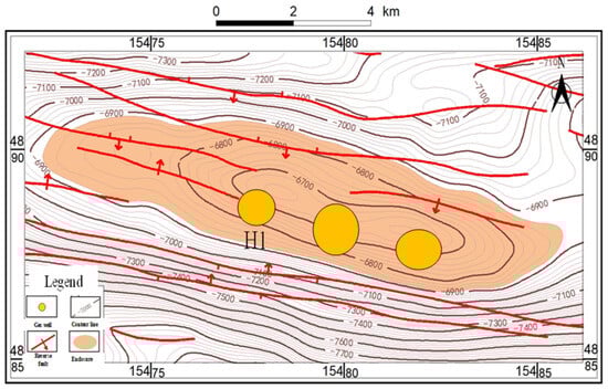
Figure 1.
Top surface structure diagram of Gas Field H.
Due to the scarcity of gas test and production wells in the well area, the lack of production capacity test data, the unclear main control factors of production capacity in the target layer, and the significant production capacity differences within the Qingshuihe Formation and Kalazha Formation layers, combined with seepage theory and production test dynamics, the productivity difference in the H1 well area is mainly controlled by the development of fractures. Moreover, as production proceeds, the pressure in the well area decreases, and the influence of in situ stress changes on the natural fractures, physical property characteristics (porosity, permeability), and production dynamics of the reservoir is unclear. Due to fewer gas test and recovery wells in the well area, the capacity test data are lacking, the main controlling factors of the capacity of the target formation are unclear.
There are still challenges in how to effectively utilize on-site data and indoor experimental results to carry out four-dimensional in situ stress research based on the integration of geology and engineering.
Therefore, we aimed at the shortcomings existing in other models. Firstly, this article conducts stress sensitivity experiments on rock samples of tight ultra-high-pressure gas reservoirs to clarify the stress sensitivity law of block reservoirs. Based on the experimental results of well logging interpretation and rock mechanic parameters, as well as the three-dimensional geological model, a three-dimensional finite element geomechanic model and a gas reservoir numerical simulation model were established. Production history fitting was carried out to obtain the variation of the pressure field in different production time blocks. The boundary conditions for pore pressure variation were set for different production times. A seepage–stress coupled four-dimensional in situ stress modeling and analysis method was proposed, and the variation law of in situ stress during the development process was predicted. Finally, the influence of considering stress sensitivity on reservoir production was simulated.
2. Stress-Sensitive Characterization of Ultra-High-Pressure Tight Sandstone Gas Reservoirs
Deep dense sandstone gas reservoirs in the Junggar Basin reflect strong stress sensitivity due to diagenesis and high levels of stress caused by geotectonic movements, which have contributed to the development of natural fractures [15,16]. In the process of gas reservoir production, the pore pressure gradually decreases with gas extraction, and the rock also deforms under the action of stress, which leads to changes in its pore structure, and the porosity and permeability of the rock decreases, which is especially obvious in fractured reservoirs [17]. In order to clarify the influence of stress sensitivity of the ultra-high-pressure reservoir on its seepage law, a stress sensitivity experiment of the gas reservoir in well area H1 was carried out, and a mathematical model was fitted based on the experimental results, which provides physical change data for production simulation. This experiment adopts the variable circumferential pressure experiment to determine the rock stress sensitivity, i.e., keep the flow pressure constant, and by changing the circumferential pressure, determine the core permeability corresponding to different effective stresses [18].
2.1. Experimental Samples and Methods
The stress sensitivity test of reservoir permeability was carried out through the high-temperature and high-pressure test system and the conventional temperature and pressure interpenetration and stress sensitivity test system. The gas used in the experiment was nitrogen (nitrogen is more stable than other gases and is less likely to undergo physical and chemical reactions with the core). The experimental sample sampling layer and parameter statistics are shown in Table 1, and the specific experimental procedures are as follows:
- (1)
- As shown in Figure 2, a core plunger with a diameter of about 2.5 cm and a length of 4.0 cm to 6.0 cm was drilled, and the end was smoothed; the length L and diameter d of the rock sample to be tested were recorded.
- (2)
- Artificial crevassing was carried out on rock samples Y-8A and Y-13A/B using Brazilian splitting experiments.
- (3)
- The permeability k of complete rock samples was directly measured by using the RSAG-1 high-temperature and high-pressure core multi-parameter measurement system, of which two groups were under normal temperature and pressure (50 MPa, 20 °C) conditions and one group was under high-temperature and high-pressure (160 MPa, 160 °C) conditions. The ambient temperature and pressure conditions were loaded with a perimeter pressure up to 5 MPa, keeping the inlet pressure constant and connecting to atmospheric pressure at the outlet end. After the determination of the first permeability, the perimeter pressure was loaded to 50 MPa at intervals of 5 MPa, and we waited for the core to stabilize for 25 min to measure the gas permeability of the core under the corresponding perimeter pressure. Under high-temperature and high-pressure conditions, the perimeter pressure was loaded to 50 MPa, keeping the inlet pressure constant and the outlet end connected to atmospheric pressure. After the first permeability was measured, the perimeter pressure was loaded to 160 MPa at 10 MPa intervals in turn, and after waiting for the core to stabilize for 25 min, the gas permeability of the core at the corresponding perimeter pressure was measured.
- (4)
- Under normal temperature and pressure conditions, after loading to 50 MPa, the enclosing pressure was unloaded to 5 MPa at intervals of 5 MPa, and after waiting for the core to stabilize for 25 min, the gas permeability of the core under the corresponding enclosing pressure was measured. Under high-temperature and -pressure conditions, after loading to 160 MPa, the enclosing pressure was unloaded to 50 Mpa at intervals of 10 Mpa, and after waiting for the core to stabilize for 25 min, the gas permeability of the core under the corresponding confining pressure was measured.
- (5)
- Steps (3)~(4) were repeated, and a second cycle of loading and unloading of the perimeter pressure was carried out again. After the aging experiments of two cycles of loading and unloading of the perimeter pressure, steps (3)~(4) were repeated again to carry out the permeability stress sensitivity experiments with changing the perimeter pressure.

Table 1.
Comparison of sampling layers and physical properties of tight sandstone experimental rock samples.
Table 1.
Comparison of sampling layers and physical properties of tight sandstone experimental rock samples.
| Samples | Stratum | Depth of Burial, m | Core Diameter, mm | Core Length, mm |
|---|---|---|---|---|
| Y-8A | K1q | 7429.95 | 24.21 | 43.23 |
| Y-13A/B | J3k | 7524.35 | 70.00 | 100.00 |
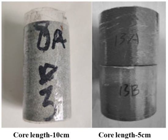
Figure 2.
Experimental rock sample diagram.
2.2. Experimental Results and Analysis
A total of three stress sensitivity experiments of rock samples from dense sandstone gas reservoirs were conducted, and the Jones stress sensitivity coefficient method was used to evaluate the degree of stress sensitivity of the rock samples; i.e., the measured experimental data were processed by Formula (1) to obtain the stress sensitivity coefficient (df) of the core and then evaluate the degree of stress sensitivity of the rock samples.
where df is the stress sensitivity coefficient (dimensionless), σef is the effective stress in MPa; K is the permeability corresponding to σef in mD, σef,0 is the effective stress at the initial measurement point in MPa, K0 is the permeability at the initial measurement point in mD. The evaluation criteria for this method classify sensitivity as weak when df ≤ 0.3, moderate when 0.3 < df ≤ 0.7, and strong when df > 0.7.
The experimental results show that the Jones stress sensitivity coefficients of rock samples Y-8A, Y-13A, and Y-13B are 0.844, 0.927, and 1.222, respectively, and the degree of stress sensitivity is strong, and the permeability of the fractured rock samples shows an obvious decreasing trend with the increase in effective stress, with a decreasing range of 55.6~99.71%. From Figure 3, it can be seen that for self-supported fractures, the permeability decreases rapidly at the beginning of the effective stress loading stage and then slows down gradually. The overall trend shows that with the increase in effective stress, the fracture gradually closes and the permeability gradually decreases. Whether under normal temperature and pressure or high temperature and pressure, the permeability cannot be fully recovered after the permeability decreases, even if the effective stress decreases again. It can be seen that stress sensitivity also produces irreversible plastic deformation on the basis of elastic deformation. Meanwhile, the effect of high-temperature and high-pressure conditions on permeability is more obvious: under the same effective stress, the permeability under high temperature and high pressure is lower than that under normal temperature and normal pressure. And with the increase in effective stress, the maximum damage rate of permeability is 84.3%, and the damage rate of irreversible permeability is 47.3%, which indicates that the permeability sensitivity is stronger in the case of high temperature and high pressure with fractures.
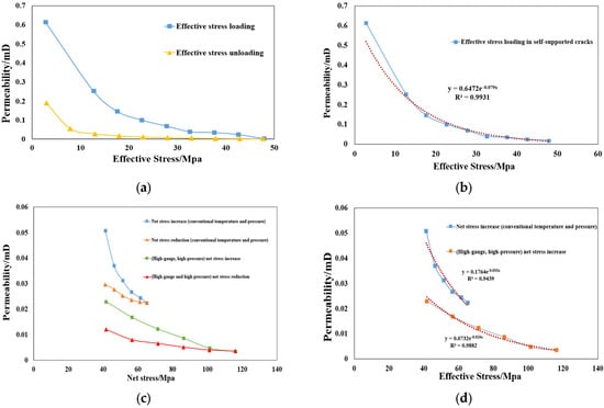
Figure 3.
Relationship between permeability and effective stress of Y-8A core and Y-13 core: (a) Effective stress loading and unloading curves. (b) Permeability and effective stress fitting results. (c) Effective stress loading and unloading curves under high-temperature and high-pressure conditions. (d) Permeability and effective stress fitting results under high-temperature and high-pressure conditions.
3. Three-Dimensional Geomechanical Modeling of Gas Reservoirs
3.1. One-Dimensional Geomechanical Characterization
In order to carry out geomechanical modeling and four-dimensional geostress simulation, it is necessary to carry out mechanical characterization of a single well, which mainly includes rock mechanical parameters, principal stress, and pore pressure.
- (1)
- Rock mechanical parameter
Through indoor rock mechanical parameter experiments, indoor experimental data were derived, and then longitudinal/transverse wave curves were fitted to calculate the rock mechanical parameters, and the two sets of data were compared and calibrated to realize parameter transformation [19]. Finally, the orthotropic mathematical model of different layers in the H1 well area was obtained, as shown in Table 2, and the model can reflect the relationship between dynamic and static parameters of rock mechanics.
Table 2.
Forward modeling mathematical models for rock mechanics parameters of different rock types in geological formations.
- (2)
- Overburden pressure
The overburden pressure is caused by the gravitational force on the rock column at the test point, and at a point of depth h, the overburden pressure is calculated by integrating the gravitational force applied above it from the surface to the depth of the point.
where σv is the overburden pressure in MPa, ρg is the rock bulk density in kg/m3, ρml is the density of the rock layer at the ground datum in kg/m3, g is the acceleration of gravity in m/s2, h is the vertical depth from the surface to the target layer in m, WD is the depth of surface water in m, A0 and b are the fitting parameters. The pressure coefficients of the overlying rock layers were directly obtained as 2.51 to 2.74 by density integration.
- (3)
- Pore pressure
Horizontal principal stresses in the formation increase and decrease as pore pressure increases and decreases [20]. The pore pressure in the article was obtained from the original pressure interpretation of early production wells and logging interpretation, and the formation pressure in the whole study area is an anomalously high pressure, with pressure coefficients ranging from 2.0 to 2.02.
- (4)
- Horizontal principal stress
Currently, the calculation methods of minimum horizontal stress at home and abroad include the formula based on logging curves and the direct measurement method. In this study, the porous elastic horizontal deformation model is used [8].
where σH and σh are maximum and minimum horizontal principal stresses in MPa, respectively; εH and εh are maximum and minimum horizontal deformations, respectively; E is Young’s modulus in MPa; ν is Poisson’s ratio; pp is pore pressure in MPa; and α is Biot’s coefficient.
Combined with the indoor experimental results for comparison and calibration, the εH and εh in the study area were obtained as 1.35 × 10⁻³ and 1.2 × 10⁻⁴, respectively, which resulted in a size range of the minimum horizontal principal stresses of about 140.6~221.5 MPa and a range of the maximum horizontal principal stresses of 181.6~258.2 MPa.
3.2. Three-Dimensional Geomechanical Modeling
The modeling process is shown in Figure 4. Before modeling, all kinds of original data (drilling, logging, and geological data) were summarized, and on the basis of the geological model, logging interpretation, etc., the three-dimensional visual modeling software Petrel RE was applied to build a three-dimensional geomechanical model of the H1 well area [21,22]. Deterministic modeling is used to establish a three-dimensional geological model based on the existing seismic interpretation and geological data and make corrections (when establishing the sand body, the sequential indicator simulation algorithm is chosen to regulate the continuity of the sand body by adjusting the value of the variance function and determining the variance function), and one-dimensional rock mechanical parameters are calculated by combining with the logging interpretation, and the one-dimensional geomechanical parameters are imported into Petrel RE, and the finite element algorithm is applied to establish a three-dimensional geomechanical model and obtain the mechanical parameters and the characteristics of stress magnitude and direction distribution.
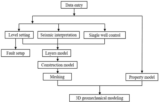
Figure 4.
Three-dimensional geomechanical modeling process diagram.
A three-dimensional geomechanical model of the H1 well area was established based on the process shown in Figure 4, in which the planar area is about 80 km2, and the depth range of modeling in the vertical direction is from −6590 m to −7480 m, divided into 100 small layers. The planar accuracy of the model is 100 m × 100 m, and the total number of grid cells in the whole area is 213 × 39 × 100 = 830,700. Combined with the logging data and indoor experimental analysis and other information, based on the one-dimensional geomechanical characterization, a three-dimensional geomechanical attribute model was established, and the attribute parameters mainly include Poisson’s ratio, Young’s modulus, maximum and minimum horizontal principal stresses, pore pressures, etc., as shown in Figure 5.
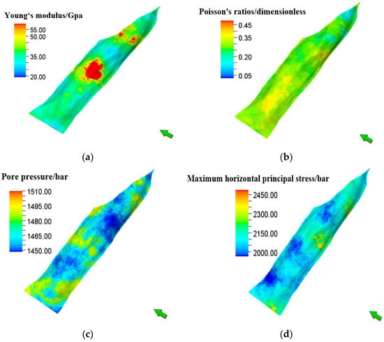
Figure 5.
Three-dimensional geomechanical modeling process diagram: (a) static Young’s modulus; (b) static Poisson’s ratio; (c) pore pressure; (d) maximum horizontal principal stress.
4. Study on the Change Rule of Four-Dimensional Ground Stress Based on the Coupling of Seepage Field and Stress Field
The four-dimensional coupled geostress simulation process in this article is shown in Figure 6: (1) Establish a three-dimensional gas reservoir numerical model of the target block based on the geologic model, and obtain the change of pore pressure with time by production history fitting. (2) Based on the 3D geomechanical model, combine the experimental model of geostress with the single well profile to form the initial stress field of the block. (3) Calculate the change field of pore pressure at different mining times as boundary conditions, and construct a four-dimensional geostress dynamic prediction model with seepage–mechanics coupling by cross iterative coupling operation with Petrel RE software.
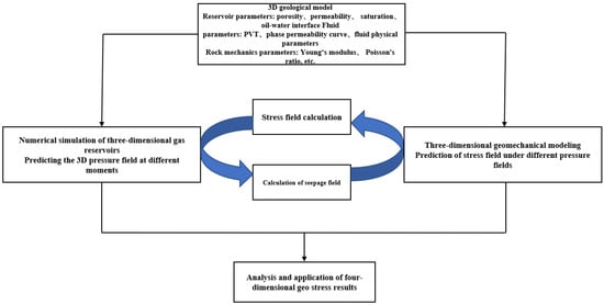
Figure 6.
Application flowchart of four-dimensional geostress coupled numerical simulation modeling.
4.1. Seepage Field–Stress Field Coupling Mechanism
There is an interaction between the seepage field and the stress field. Changes in the stress field can lead to alterations in the pore structure of rocks, thereby affecting the seepage characteristics. During the seepage process, the pressure change of the fluid will in turn act on the rock skeleton, causing the adjustment of the stress field. This interaction needs to be accurately described by establishing a coupled mathematical model [23,24,25]. The following are the mathematical modeling methods:
4.1.1. Seepage Field Equation
For a linearly elastic solid, the following equilibrium equations are satisfied:
Assuming that the reservoir rock deformation satisfies the linear elasticity criterion, the principle of effective stress can be written as
where is the total stress in MPa, is the effective stress in MPa, [mij] is the Kroneker tensor, p is the pore pressure in MPa, α is the Biot’s coefficient, and Fi is the body force, which is defined as
where KT is the bulk modulus of the equivalent material (solid phase plus pores) in GPa, Ks is the bulk modulus of the solid phase in GPa.
The eigenstructural equations expressed using effective stresses are as follows:
where [D] is the effective principal matrix, and is the elastic strain, which can be expressed in terms of rock displacement:
The Lamé coefficients λ and µ are defined as
where E is Young’s modulus in GPa, and v is Poisson’s ratio, which is dimensionless.
It can be obtained from the above equation by the following association:
The above equation is the rock deformation model, where is the Hamiltonian operator, and is the Laplace operator.
4.1.2. Stress Field Equation
Assuming that the fluid percolation process in the pore medium follows Darcy’s law, without considering the influence of the fluid’s own gravity and temperature change, the continuity equation of gas–water two-phase percolation can be obtained by the law of conservation of mass:
where subscript l denotes gas or liquid phase, subscript pm denotes matrix or fracture, ϕl,pm is porosity, krl,pm is relative permeability in mD, ul,pm is fluid viscosity in mPa s, pl,pm is fluid pressure in mPa·s, ρl,pm is fluid density in kg/m3, Sl,pm is fluid saturation, Bl,pm is the fluid volume coefficient, g is gravitational acceleration in kg·m/s2, H is vertical elevation in m, and Ql,pm is fluid cumulative term.
The gas–water two-phase saturation and capillary force equations are as follows:
4.1.3. Coupling Model
The iterative method is adopted to handle the coupling of seepage and stress fields. Firstly, given the initial stress field or seepage field, solve the equation of one of the fields to obtain the distribution of that field. Then, substitute the result of this field as the boundary condition or source term into the equation of another field to solve for the other field. Repeat this iteration repeatedly until the convergence condition is met.
4.1.4. Seepage–Stress Coupling Mechanism
In the process of seepage–stress coupling, the fluid pressure change affects the effective stress acting on the rock skeleton, leading to the deformation of the rock body. The deformation of the rock body changes the rock pore space, which in turn changes the porosity and permeability of the reservoir, and thus affects the flow of the fluid [22]. In the coupled model used in this article, the time domain of the seepage model is firstly divided into multiple time steps, and in one time step, the seepage model is firstly solved, and the results of the seepage model (pore pressure, etc.) are transferred to the rock mechanics model to calculate the deformation and stress change of the rock body in the present time step, and then the porosity and permeability are updated and passed back to the seepage model for calculation in the next time step [9].
According to the Carman–Kozeny formula, permeability is closely related to porosity. Then, the porosity and permeability stress sensitivity model [11] can be expressed as follows:
where ϕ0 is the initial porosity, and k0 is the initial permeability.
By establishing an accurate coupling mathematical model of the seepage and stress field, complex physical phenomena in underground engineering can be better understood and predicted, providing a scientific basis for engineering design and decision-making.
4.2. Production History Fitting
Since the dew-point pressure of the reservoir is much smaller than the formation pressure under the reservoir pressure and temperature conditions, the gas–water two-phase black oil model was chosen for this simulation, in which the relative permeability of gas and water and the sensitive fitted model curves of reservoir pressure are shown in Figure 7 (these relative permeability rates were obtained through experiments using a phase permeability meter; the used gas is also nitrogen). In order to match the actual situation as much as possible, the constructed model were fitted with history. Under the condition of constant gas production, the historical fitting of wellbore flow pressure was carried out, and parameters such as porosity and permeability were adjusted to obtain the single-well fitting curves as shown in Figure 8 and Figure 9.
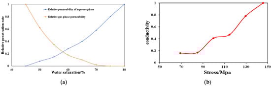
Figure 7.
Curve of fitting model for gas water relative permeability and reservoir stress sensitivity: (a) Relative permeability curves of gas and water. (b) Reservoir stress-sensitive fitting model curves.
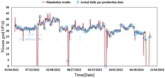
Figure 8.
H1 well daily gas production fitting curve.
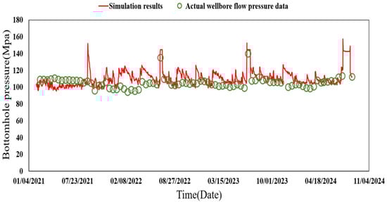
Figure 9.
H1 well bottom flow pressure fitting curve.
4.3. Simulation of Four-Dimensional Geostress Change Patterns in Production Processes
Based on the established three-dimensional geomechanical model, Petrel RE was used to calculate the initial in situ stress values, thereby obtaining that the primary value distribution of the initial maximum horizontal principal stress in the target area was 160–260 MPa, the minimum horizontal principal stress was 125–225 MPa, and the vertical stress was 150–200 MPa. The horizontal stress difference was 15 to 55 MPa. The average value of the maximum horizontal principal stress recorded in the on-site data was 215 MPa, and the average value of the minimum horizontal principal stress was 173 MPa.
Then, the three-dimensional in situ stress parameters were compared, respectively, with the one-dimensional in situ stress parameters and the on-site data: (1) Compared with the one-dimensional in situ stress parameters (as shown in Figure 10), the fitting effect was better. (2) Compared with the on-site data, the average error of the maximum horizontal principal stress was 2.38%, and the average error of the minimum horizontal principal stress was 1.16%. By comparing the three-dimensional data with the one-dimensional data and the on-site data, respectively, the error results were all small, indicating that the fitting effect was good, thereby determining the accuracy of the model.
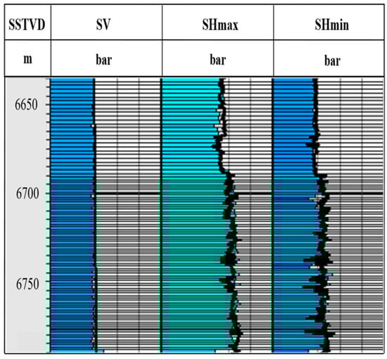
Figure 10.
Initialization stress comparison chart.
Three gas extraction wells were set up at 1 km, 1.3 km, and 1.6 km away from the H1 well, and the total gas extraction rate was set to 1.2 million m3/day based on the production history fitting for a 20-year production prediction simulation.
4.3.1. Characteristics of Pore Pressure Variation
Figure 11 shows the pore pressure change process during the simulated production from 2025 to 2045, which shows that the pore pressure gradually decreases after a period of production, and a pressure drop funnel is formed around each well. After 20 years of production, the pore pressure decreases from 127.55~151.77 MPa to 77.68~151.51 MPa.
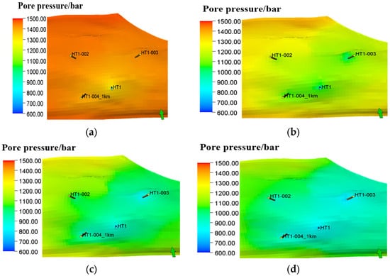
Figure 11.
Pore pressure variation diagram during the production process from 2025 to 2045: (a) Pore pressure variation during production in August 2025. (b) Pore pressure variation during production in August 2030. (c) Pore pressure variation during production in August 2037. (d) Pore pressure variation during production in August 2045.
4.3.2. Characteristics of Changes in the Magnitude of Horizontal Principal Stresses
Figure 12 and Figure 13 show the variation of the maximum/minimum horizontal principal stresses in the reservoir during the simulated production from 2025 to 2045. As production proceeds, the maximum/minimum horizontal principal stress in the reservoir gradually decreases. The maximum horizontal principal stress of the reservoir in the block decreases from 140.35~436.51 MPa to 130.73~434.03 MPa; the minimum horizontal principal stress decreases from 103.29~384.74 MPa to 89.53~383.05 MPa. Meanwhile, combining with the pore pressure distribution graph, it can be seen that the greater the pressure drop around the well, the greater the change in the maximum/minimum principal stress.
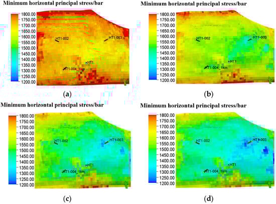
Figure 12.
Minimum principal stress variation diagram during the production process from 2025 to 2045: (a) Minimum principal stress changes during production in August 2025. (b) Minimum principal stress variation during production in August 2030. (c) Minimum principal stress variation during production in August 2037. (d) Minimum principal stress variation during production in August 2045.
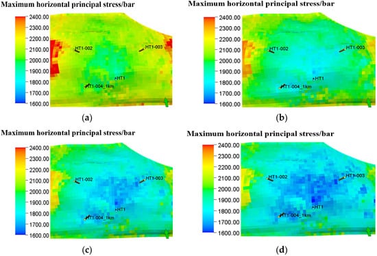
Figure 13.
Maximum principal stress variation diagram during the production process from 2025 to 2045: (a) Maximum principal stress variation during production in August 2025. (b) Maximum principal stress variation during production in August 2030. (c) Maximum principal stress variation during production in August 2037. (d) Maximum principal stress variation during production in August 2045.
4.3.3. Characteristics of Changes in the Direction of Principal Stress
Figure 14, Figure 15 and Figure 16 show the direction distribution of maximum/intermediate/minimum principal stresses in the reservoir for 20 years of production. At the beginning of production, the maximum principal stress is mostly NE71° and the minimum principal stress is mostly NW19°. After 20 years of production, it can be found that in some areas around the four wells, the direction of the maximum principal stress changes to a vertical direction. The intermediate principal stress with the direction of NW19° first changes to a vertical direction, and then it changes to a horizontal NE direction, with a maximum deflection angle of 90°. The minimum principal stress in the vertical direction is gradually deflected to horizontal NW19°.
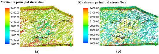
Figure 14.
Variation diagram of maximum principal stress direction during the production process from 2025 to 2045: (a) Change in direction of maximum principal stresses during production in August 2025. (b) Change in direction of maximum principal stresses during production in August 2045.
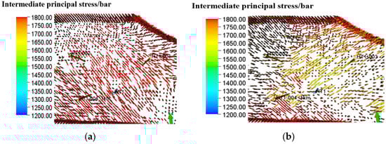
Figure 15.
Variation diagram of intermediate principal stress direction during the production process from 2025 to 2045: (a) Change in direction of intermediate principal stresses during production in August 2025. (b) Change in direction of intermediate principal stresses during production in August 2045.

Figure 16.
Variation diagram of minimum principal stress direction during the production process from 2025 to 2045: (a) Change in direction of minimum principal stresses during production in August 2025. (b) Change in direction of minimum principal stresses during production in August 2045.
Finally, the change curves of permeability and porosity with formation pressure obtained by combining the high-temperature and high-pressure stress-sensitive experimental data processing and the prediction results of the development scheme without considering the stress-sensitive effect were compared and analyzed, as shown in Figure 17. Under the influence of the stress-sensitive effect, the time of stable production of the wells was reduced, and the cumulative gas production was reduced. Therefore, it is necessary to take the stress-sensitive effect into consideration to formulate a reasonable production plan for ultra-high-pressure tight gas reservoirs.
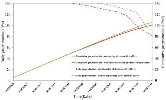
Figure 17.
Comparison of predicted results for development scenarios with and without consideration of stress sensitivity effects.
5. Conclusions
- (1)
- The results of stress-sensitive experiments on dense sandstone of the gas reservoir in the H1 well area show that, whether under normal temperature and pressure or high-temperature and high-pressure conditions, with the increase in effective stress, self-supporting fractured rock samples will show a stress-sensitive effect, and with the increase in stress, permeability decreases fast at the beginning and then becomes slower gradually. Even if the effective stress is reduced, the reservoir permeability cannot be fully recovered, and the effect of high-temperature and high-pressure conditions on permeability is more significant. It shows that the permeability sensitivity is strong under high temperature and high pressure with fractures.
- (2)
- A four-dimensional in situ stress numerical simulation method suitable for seepage–stress coupling in tight sandstone gas reservoirs was proposed. Compared with traditional methods, this method is based on actual production data and truly reflects the changes in in situ stress in the actual production process. Secondly, considering the influence of reservoir stress sensitivity and heterogeneity, the simulation results have a high degree of consistency with the actual development dynamics. When this method is applied to the calculation of the initial in situ stress in the target block, the result has a high degree of consistency with the measured in situ stress value of a single well, verifying the accuracy of the four-dimensional in situ stress model.
- (3)
- During the dynamic production process, the results of in situ stress analysis indicated that after 20 years of mining, the pore pressure in the target block decreased by approximately 50 MPa, the maximum horizontal principal stress decreased by approximately 2.5–10.7 MPa, and the minimum horizontal principal stress decreased by 2.7–14.2 MPa. Near the production well periphery, the in situ stress deflects, and near the well periphery with higher production, the direction deflection of the in situ stress is more obvious. The research results can provide temporal stress field distribution results for the simulation and prediction of the secondary fracturing of old wells and the commissioning fracturing of new wells in the target well area.
- (4)
- A 20-year analysis of the production effects of gas wells considering stress sensitivity and not considering stress sensitivity was carried out. The simulation shows that, due to the influence of the stress sensitivity effect, the stable production time of gas wells is reduced and the cumulative gas production decreases. For ultra-high-pressure tight gas reservoirs, the stress sensitivity effect needs to be considered, and a more reasonable production allocation plan needs to be formulated subsequently.
Author Contributions
Conceptualization, C.Z. and L.S.; methodology, H.S. and L.S.; software, L.Y. and P.Q.; validation, S.L. and Y.L.; investigation, Y.L. and C.Z.; writing—original draft preparation, S.L.; writing—review and editing, Y.L. and Y.H. All authors have read and agreed to the published version of the manuscript.
Funding
This research was funded by the Natural Science Foundation of China (No. 52304044) and the Science and Technology Cooperation Project of the CNPC-SWPU Innovation Alliance (No. 2020CX010403).
Data Availability Statement
Data are contained within the article.
Conflicts of Interest
Authors Chuankai Zhao, Lei Shi, Hang Su, Liheng Yan, Peng Qiu, and Yuanwei Hu were employed by the company PetroChina Xinjiang Oilfield. The remaining authors declare that the research was conducted in the absence of any commercial or financial relationships that could be construed as a potential conflict of interest. The authors declare that this study received funding from the Science and Technology Cooperation Project of the CNPC-SWPU Innovation Alliance. The funder was not involved in the study design, collection, analysis, interpretation of data, the writing of this article, or the decision to submit it for publication.
References
- Liu, Y.J.; Zhu, H.Y.; Tang, X.H.; Sun, H.; Zhang, B.; Chen, Z. Four-dimensional in-situ stress model of CBM reservoirs based on geology– engineering integration. Nat. Gas Ind. 2022, 42, 82–92. [Google Scholar]
- Wang, Z.M.; Zhang, H.; Xu, K.; Wang, H.; Liu, X.; Lai, S. Key technology and practice of well stimulation with geology and engineering integration of ultra-deep fractured sandstone gas reservoir. China Pet. Explor. 2022, 27, 164–171. [Google Scholar]
- Niu, S.W. Research and application of geology and engineering integration for low-permeability tight oil reservoirs in Shengli Oilfield. China Pet. Explor. 2023, 28, 14–25. [Google Scholar]
- Wang, T.; Yan, X.; Yang, X.; Yang, H. Dynamic subsidence prediction of ground surface above salt cavern gas storage considering the creep of rock salt. Sci. China Technol. Sci. 2010, 53, 3197–3202. [Google Scholar] [CrossRef]
- Rutqvist, J. Status of the TOUGH-FLAC simulator and recent applications related to coupled fluid flow and crustal deformations. Comput. Geosci. 2011, 37, 739–750. [Google Scholar] [CrossRef]
- Teufel, L.W.; Rhett, D.W. Geomechanical evidence for shear failure of chalk during production of the Ekofisk Field. In Proceedings of the 66th Annual Technical Conference and Exibition, Dallas, TX, USA, 6–9 October 1991. [Google Scholar] [CrossRef]
- Tang, X.H. Multi-Physics Based 4D Stress Evolution of Shale Gas Reservoir. Ph.D. Thesis, Southwest Petroleum University, Chengdu, China, 2020. [Google Scholar]
- Zhu, H.Y.; Song, Y.J.; Xu, Y.; Li, K.; Tang, X. Four-dimensional in-situ stress evolution of shale gas reservoirs and its impact on infill well complex fractures propagation. Acta Pet. Sin. 2021, 42, 1224–1236. [Google Scholar]
- Zhu, H.Y.; Song, Y.J.; Lei, Z.D.; Tang, X. 4D-stress evolution of tight sandstone reservoir during horizontal wells injection and production: A case study of Yuan 284 block, Ordos Basin, NW China. Pet. Explor. Dev. 2022, 49, 136–147. [Google Scholar] [CrossRef]
- Yang, J.W.; Jia, S.P.; Fu, X.F.; Xu, M.; Zhang, G.; Wang, Z.; Wu, G. 4D geomechanical analysis of geological bodies in abnormally high pressure exhausted gas storage: A case study of Southwest X gas storage. Chin. J. Rock Mech. Eng. 2023, 42, 4189–4203. [Google Scholar]
- Xi, Z.Q.; Jia, S.P.; Wang, X.W.; Zhang, P.J.; Bi, Y.; Zhang, B. Analysis of the pressure-bearing capacity of carbonate reservoirs for gas storage based on four-dimensional dynamic geomechanics. Xinjiang Oil Gas 2024, 20, 63–70. [Google Scholar]
- Zheng, J.; Zheng, L.; Liu, H.-H.; Ju, Y. Relationships between permeability, porosity and effective stress for low-permeability sedimentary rock. Int. J. Rock Mech. Min. Sci. 2015, 78, 304–318. [Google Scholar] [CrossRef]
- Liu, J.L. Study on the Distribution of Sedimentary Systems and Favorable Reservoir Facies Zones in the Lower Assemblage of the Southern Margin of the Junggar Basin (Kalaza Formation—Qingshuihe Formation). Master’s Thesis, Yangtze University, Jingzhou, China, 2023. [Google Scholar]
- Kang, Y.-L.; Li, C.-J.; You, L.-J.; Li, J.-X.; Zhang, Z.; Wang, T. Stress sensitivity of deep tight gas-reservoir sandstone in Tarim Basin. Nat. Gas Geosci. 2020, 31, 532–541. [Google Scholar]
- Xu, C.C.; Zou, W.H.; Yang, Y.M.; Duan, Y.; Shen, Y.; Luo, B.; Ni, C.; Fu, X.D.; Zhang, J.Y. Status and prospects of exploration and exploitation of the deep oil and gas resources onshore China. Nat. Gas Geosci. 2017, 28, 11391153. [Google Scholar]
- Liao, X.W.; Wang, X.Q.; Gao, W.L. Study on stress sensitivity of permeability for deep gas reservoirs in Talimu. Nat. Gas Ind. 2004, 24, 93–94. [Google Scholar]
- Xiao, W.L.; Li, M.; Zhao, J.Z.; Zheng, L.L.; Li, L.J. Laboratory study of stress sensitivity to permeability in tight sandstone. Rock Soil Mech. 2010, 31, 775–779. [Google Scholar]
- Zhao, Y.C.; Luo, Y.; Li, L.X.; Zhou, Y.; Li, L.M.; Wang, X. In-situ stress simulation and integrity evaluation of underground gas storage: A case study of the Xiangguosi underground gas storage, Sichuan, SW China. J. Geomech. 2022, 28, 523–536. [Google Scholar]
- Liang, H.S.; Wen, G.F.; Wang, G.H.; Zhang, Y.Z.; Cheng, Y.F.; Zhao, J.H. Study on the influence of pore pressure variation on ground stress. Pet. Drill. Tech. 2004, 32, 18–20. [Google Scholar]
- Lei, D.W.; Chen, N.G.; Li, X.Y.; Zhang, Y.C. The major reservoirs and distribution of lower combination in southern margin of Junggar basin. Xinjiang Pet. Geol. 2012, 33, 648–650. [Google Scholar]
- Cai, M.H.; Hu, D.X.; Pu, G.Q.; Fan, J.H.; Wang, Z.H.; Yi, S.H.; Ma, Y.M.; Chen, X.H. Approach to prediction method for tectonic stress compensating formation pressure. Xinjiang Pet. Geol. 2012, 33, 507–508. [Google Scholar]
- Zhang, D.; Zhang, L.; Tang, H.; Zhao, Y. Fully coupled fluid-solid productivity numerical simulation of multistage fractured horizontal well in tight oil reservoirs. Pet. Explor. Dev. 2022, 49, 338–347. [Google Scholar] [CrossRef]
- Tan, X.-H.; Zhou, X.-J.; Xu, P.; Zhu, Y.; Zhuang, D.-J. A fractal geometry-based model for stress-sensitive permeability in porous media with fluid-solid coupling. Powder Technol. 2025, 455, 120774. [Google Scholar] [CrossRef]
- Liu, G.; Shang, D.; Zhao, Y.; Du, X. Characterization of brittleness index of gas shale and its influence on favorable block exploitation in southwest China. Front. Earth Sci. 2024, 12, 1389378. [Google Scholar] [CrossRef]
- Zhang, L.; Yuan, X.; Luo, L.; Tian, Y.; Zeng, S. Seepage characteristics of broken carbonaceous shale under cyclic loading and unloading conditions. Energy Fuels 2023, 38, 1192–1203. [Google Scholar] [CrossRef]
Disclaimer/Publisher’s Note: The statements, opinions and data contained in all publications are solely those of the individual author(s) and contributor(s) and not of MDPI and/or the editor(s). MDPI and/or the editor(s) disclaim responsibility for any injury to people or property resulting from any ideas, methods, instructions or products referred to in the content. |
© 2025 by the authors. Licensee MDPI, Basel, Switzerland. This article is an open access article distributed under the terms and conditions of the Creative Commons Attribution (CC BY) license (https://creativecommons.org/licenses/by/4.0/).