Abstract
As the fundamental analytical tool of the integrated electricity–heat–gas energy system (IEHGES), static energy-flow calculation (EFC) can be implemented repeatedly to arbitrary IEHGESs, imposing higher demands on the universality and efficiency of the EFC framework. Therefore, this paper proposes a matrix-based universal EFC framework for IEHGES. Standardized modeling of individual subnetworks is first conducted. On this basis, the iterative matrices with gradient-descent direction are then derived from the established subnetwork models. Both the energy-flow models and the iterative matrices are expressed in compact matrix form. After that, according to the coupling chain-based interdependency mechanism analysis method of IEHGES, the Newton–Raphson-based universal EFC framework is developed. By inputting system parameters in a given data format, the state of arbitrary IEHGESs can be automatically calculated through the proposed EFC framework. The simulation results using two test systems with different scales verify that the proposed framework offers advantages over existing methods in portability and robustness, and its highest computational efficiency is approximately 2 and 2.3 times that of traditional methods for medium and large test systems, respectively.
1. Introduction
Over the past few decades, fragmented and suboptimal energy utilization has resulted in the rapid depletion of fossil fuels and the excessive emission of greenhouse gases, leading to a severe ecological and environmental crisis [1]. To meet this challenge, the integrated electricity–heat–gas energy system (IEHGES) has been widely promoted and deployed [2]. Distinguishing from the conventional energy infrastructure, IEHGES enables complementarities and synergies between heterogeneous energy resources by coupling different energy systems through energy-conversion devices, thus improving the efficiency and flexibility of energy management [3]. As an effective analytical tool for quantifying the interdependency within IEHGES, the steady-state energy-flow calculation (EFC) provides a rapid state snapshot of IEHGES at a given time step, and it has been widely applied in the long-term collaborative planning, economic dispatch, and security assessment of IEHGES [4].
Focusing on the energy-flow modeling and model solution strategy, numerous studies have been conducted on the EFC framework of IEHGES [5]. Nevertheless, most of the current research accomplishments remain largely theoretical, making them inadequate for engineering deployment. On the one hand, the portability of existing energy-flow models is limited due to their case-specific nature. The effectiveness of these models cannot be assured if the physical system changes. On the other hand, the coupling mode of IEHGES determined by the operation status of energy devices has often been fixed in prior studies, limiting the universality of the corresponding EFC solution strategies for diverse interdependencies. Last but not least, the traditional framework formulations are mostly presented in a recursive form with redundant intermediate variables, which is neither concise nor computationally friendly. Therefore, investigations on standardized modeling and solution approaches are desired to develop a universal steady-state EFC tool for IEHGES with which the energy-flow analysis of arbitrary IEHGESs can be easily implemented.
The IEHGES consists of coupling devices and energy subnetworks. The energy hub (EH) concept was introduced to describe the collection of coupling devices [6], where the interactions between energy subnetworks were abstracted to a universal coupling matrix. To pragmatize this concept, several versions of standardized modeling methods have been proposed in [7,8], with which the energy flow of EH can be compactly automated into a matrix. However, the above studies only focused on EH itself, the detailed state of another important component of IEHGES—energy subnetworks—was ignored. Typically, the district electricity network (DEN), district heat network (DHN), and district gas network (DGN) constitute the subnetworks of IEHGES. Compared to others, studies on DEN models have been quite in-depth. As the mainstream model, the alternating current (AC) model portrays the operation state of the DEN with a set of nonlinear algebraic equations (AEs). The AC model is streamlined into a universal matrix form by introducing the nodal admittance matrix. To solve this model, the holomorphic embedded (HE) method [9], Gauss–Seidel method, fast decoupled load-flow method [10], etc. were developed, among which the Newton–Raphson (NR) algorithm [11] and its variants have been widely adopted due to their robustness and quadratic convergence. In [12], the matrix-based concise formula of an NR iterative matrix was directly derived from the streamlined AC model to avoid the traditional cumbersome expression form, realizing the standardized modeling and solution of the DEN model. The same EFC framework has been employed in commercial software such as MATPOWER [13], demonstrating its practicality for engineering applications.
Since DHN transmits mass flow and thermal energy simultaneously, the DHN model is divided into hydraulic and thermal parts. The universal matrix form of the hydraulic model can be derived using graph theory [14]. Specifically, there are three versions of hydraulic models, i.e., a branch-flow model (BFM) [15], a nodal-pressure model (NPM) [16], and a pressure-flow model (PFM) [17]. In contrast to other models, BFM balances the initial condition sensitivity and solution efficiency when iterative solution approaches are applied, and it is thus broadly utilized for IEHGES modeling. As for the thermal part, a pseudo-dynamic thermal model that ignores the temperature variation over time was built. Due to the directional thermal power transmission, the thermal model was usually represented as a set of mixture-temperature equations in recursive form. Recently, the matrix-based thermal models for quality-regulated and quantity-regulated DHN were derived in [18,19] and [20,21,22], respectively, laying the foundation for the standardized thermal model. However, these models are not inapplicable to arbitrary DHN topologies since their intrinsic nature cannot be strictly aligned with the original model. Additionally, models in any form fail to tackle the reversed mass flow (RMF) problem [23,24], which further undermines their universality. According to model complexity, different EFC solution strategies have been used. Gauss elimination and LU factorization were adopted to linearly calculate the decoupled thermal model [19], which are effective but scene-limited. A HE-based, non-iterative approach was raised to solve the whole DHN model in [22]. Although it takes advantage of analyticity, its reported superior convergence is subjected to suitable initial guesses generated via iterative methods. In comparison, the NR-based method remains the most prevalent, but its iterative matrix for DHN is either manually derived [25] or incompletely generated from the flowchart [15], which yields huge influences on the performance of the NR-based EFC framework. Hence, there are still some research gaps in the standardized modeling and solution of the DHN model that warrant further exploration.
To date, vast types of gas energy-flow models have been proposed for different research purposes, but they are hardly compatible with each other. On the one hand, most of the available studies have only considered the hydraulic parts of gas networks. Similar to DHN, the formulations of gas hydraulic models can also be divided into BFM [26], NPM [25], and PFM [27]. Aside from the model type, existing hydraulic models varied significantly in modeling gas compressors. The gas hydraulic model of IEHGES was established in [16] while the compressor model was ignored. For those gas-network models that contained compressors [9,22,25,28,29,30], the compressors were usually modeled to operate in a constant-compression-ratio mode. To enhance the universality of gas compressor modeling, an IEHGES model considering three operation modes of compressors was proposed in [31]. However, the difference in compressor-driving modes was still neglected. On the other hand, the widespread injection of alternative gas, such as hydrogen (H2) and synthetic natural gas (SNG), has led to increasingly complex gas properties in DGN, significantly impacting the gas energy flow. The simulation method of gas networks with hydrogen injections was first proposed in [32], where both gas density and gross calorific value (GCV) varied with the gas composition. On this basis, DGN models containing heterogeneous gas sources were established for the NR-based EFC and optimal EFC in [28] and [33], respectively. Since gas composition calculation depended on the gas-flow direction, the aforementioned models were represented using either flowcharts or recursive AEs, and the related iterative matrices were incompletely and manually derived. Additionally, although a compact DGN model considering hydrogen blending was formulated in [34] based on the gas admittance matrix, compressors were ignored, and its implementation was still spatially and temporally inefficient since abundant dense matrices and matrix operations were involved. In sum, it is critical yet challenging to achieve a concise formulation and efficient computation of the DGN model while ensuring its universality.
The EFC solution approaches of IEHGES can be categorized as either integrated or disaggregated. The specific implementation of either approach relies on determining the coupling mode, but most of the current EFC methods were dedicated to certain preconfigured coupling modes, which lack portability. To address this issue, four typical coupling modes were classified in [4] for an interaction analysis of IEHGES. Based on the operation modes of electricity–heat-coupling devices, the calculation sequence of the decomposed approach was classified into three types [35]. In [19], six coupling modes of the integrated electricity–heat system were sorted out through permutation and combination. All the existing determination algorithms were designed from the perspective of distinguishing specific devices. Given the vast number of possible combinations of coupling devices, those algorithms are evidently insufficient, resulting in the shallow revelation of the interdependency mechanism of IEHGES.
The taxonomy of the above literature is presented in Table 1 for a more intuitive comparison and analysis.

Table 1.
Literature reviews on the modeling and solution strategies of EFC for the integrated energy system.
Inspired by [13], this paper aims to develop a universal framework for the automatic EFC of IEHGES. Unlike previous studies that overwhelmingly focused on enhancing the performance of energy-flow analysis through solution strategy improvements, this work was conducted from the perspective of revising and reformulating the EFC model (including the subnetwork model and its iterative matrix). Additionally, the interdependency mechanism of IEHGES is comprehensively elucidated in terms of the nature of coupling relationships. Depending on the imported system parameters, the steady-state analysis of IEHGES can be carried out automatically and efficiently under the proposed framework. The main contributions of this paper include the following:
- Building upon the proposed generalized heat energy-flow direction, a standardized DHN model is formulated in a compact matrix representation, which is applicable to arbitrary heat networks with precision. By circumventing the RMF problem, its convergence domain is inherently broadened.
- A novel matrix-based DGN model consisting of hydraulic and composition-tracking models is constructed in a standardized manner in which the diversity of gas-network components is comprehensively considered. The varying gas-compressibility factor is first incorporated into the static EFC of IEHGES, and its impact on the overall system state is fully demonstrated.
- The iterative matrices of the proposed models are derived while ensuring conciseness and sparsity. All iterative matrices follow the gradient-descent direction and can be obtained directly through matrix operations, thereby improving the efficiency of the NR-based EFC process.
- A coupling chain-based analysis method that fully reveals the interdependency mechanism of IEHGES under any combination of coupling devices is proposed, ensuring the automatic execution of an NR-based universal EFC framework for any IEHGES configuration.
In addition to its contributions to energy-flow analysis, the proposed methodology provides significant advantages for other research aspects of IEHGES in which the rapid and repetitive formulation of the energy-flow models or the iterative matrices is required. The application prospects of such standardized modeling methodology include, but are not limited to, optimal EFC, probabilistic EFC, stability analysis, and a risk assessment of IEHGES.
The remainder of this article is arranged as follows. The matrix-based IEHGES model is derived in Section 2. The iterative matrices are compactly formulated in Section 3. In Section 4, a universal EFC framework is proposed based on the thorough discussion of the interdependency mechanism of IEHGES. Then, Section 5 analyzes the effectiveness of the proposed framework by case studies. Finally, Section 6 concludes this article.
2. Matrix Model Formulation of IEHGES
As depicted in Figure 1, the DEN, DHN, and DGN constitute the energy transmission network of IEHGES. All typical energy-conversion devices that interconnect subnetworks are considered, including combined-heat-and-power (CHP) units, gas turbine generators (GTGs), heat pumps (HPs), electric boilers (EBs), gas boilers (GBs) and power-to-gas (P2G) units. The proposed matrix-based modeling method is described as follows.
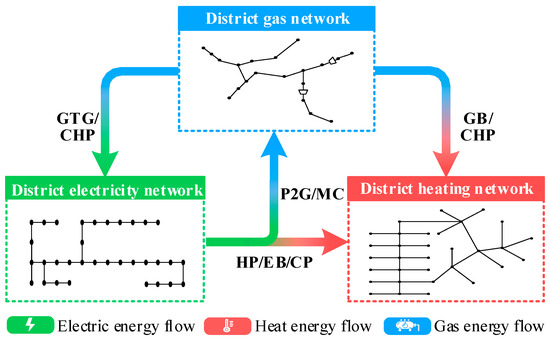
Figure 1.
Energy-flow diagram of the IEHGES.
2.1. Electricity Network Formulation
The well-known AC power flow model is utilized for the matrix formulation of the DEN. The DEN buses are classified into PQ, PV, and θV types. Since the equilibrium of power flow should be achieved at each bus, the nodal balance equations of active and reactive power are denoted as follows:
where the following applies: |Vi|/θi is the voltage magnitude/angle of bus i; θij = θi − θj; Ne is the bus number; Gij/Bij are the conductance/susceptance of electrical branch ij; is the set of PQ/PV buses; PS,i/PL,i is the active source/load power at bus i, while QS,i/QL,i is the reactive source/load power at bus i. By introducing the nodal admittance matrix Y, Equation (1) can be rewritten in a compact matrix form as follows:
where V, PS, PL, QS, and QL are the vector forms of V, PS, PL, QS, and QL, respectively; Real⟨·⟩/Imag⟨·⟩ represents the real/imaginary part of a complex expression; ‘·’ indicates the Hadamard product operation; (·)* denotes the conjugate operation.
2.2. Heating Network Formulation
A typical DHN comprises heat sources, heat loads, a supply network, and a return network, as shown in Figure 2a. According to the mass flow direction through each node, node temperatures are divided into inflow and outflow temperatures. DHN nodes are categorized into three types: (1) slack source node with specified head pressure and inflow supply temperature (hTS node); (2) ordinary source nodes with specified inflow supply temperature and power (ΦTS node); (3) non-source nodes with specified inflow return temperature and power (ΦTR node). So far, the classic recursive [15] and several matrix-based [20,21,22] DHN models have been developed. However, these models are tailored to specific networks, resulting in limited generality. A few common drawbacks of these traditional models, which are rarely discussed, can be summarized as follows:
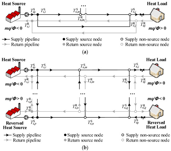
Figure 2.
Schematic diagram of the DHN. (a) Conventional schematic diagram of the DHN; (b) generalized schematic diagram of the DHN.
- The outflow supply temperature of hTS and ΦTS nodes is defaulted to the specified inflow supply temperature, , in traditional models. As depicted in Figure 2b, once the heating node i functions simultaneously as both a source node and a mixture node, the outflow temperature, , may differ from . Similarly, the outflow temperature, , may not equal the specified load inflow temperature, , if mass flow mixing occurs.
- The formulation of the nodal temperature equation is a lack of automation in traditional models. The incorrect assignment of outflow supply temperature (as described above) results in the omission of nodal temperature equations for supply source nodes. Additionally, part of the nodal temperature equations for return nodes are either manually derived from the given topology [15] or depend on node-type judgment [21,22], making them less adaptable to arbitrary DHNs.
- Current DHN models are unidirectional, with the supply mass flow direction fixed from source to load (opposite in the return network). Nevertheless, as illustrated in Figure 2b, mass flow reversal of pipelines, sources, or loads, i.e., the so-called RMF problem, is commonplace during the EFC process [16,23,36], leading to violation of energy conservation law and even no convergence in existing thermal models.
Aiming at the standardized modeling and programming of the DHN, a compact matrix-based model is constructed, which is described as the unification of hydraulic and thermal models as follows.
2.2.1. Hydraulic Model
Herein, the widely adopted BFM is formulated. According to the mass flow conservation law, the nodal mass flow balance equation of the supply network can be written in matrix form:
where the following applies: Ah is the node-branch incidence matrix; m is the pipeline mass flow vector; mq is the nodal mass flow vector. The supply and return networks are considered symmetrical, with the same mass flow values but opposite signs.
The mass flow balance equation effectively depicts the mass flow distribution in radial networks, but it is insufficient for addressing meshed networks. Thus, the loop pressure equation is introduced. Owing to the friction between the transmission medium and pipeline wall, the sum of pressure drops along a closed loop should be zero:
where Bh is the loop-branch incidence matrix, and Kh is the pipeline resistance coefficient vector, whose value is detailed in [15].
2.2.2. Thermal Model
Since the thermal energy is exchanged with sources and loads at source and non-source nodes, respectively, the nodal heat power balance equation is formulated as follows:
where the following applies: Cp is the specific heat of the transmission medium; the superscript S/R denotes the supply/return network; / is the outflow temperature vector of supply non-source/return source nodes; / is the specified inflow temperature vector of supply/return nodes; and Φn/Φs is the consumed heat power vector of non-source/source nodes.
According to the temperature-drop equation, the mass flow temperature decreases exponentially along the pipeline:
where the following applies: / is the temperature at the outlet/inlet of pipeline k; Ta,k, λh,k, Lh,k and mk are the ambient temperature, heat transfer coefficient, length, and mass flow of pipeline k, respectively; and is the DHN pipeline set. For brevity, − Ta,k and − Ta,k are denoted as ′ and ′ in Equation (6), respectively. Under the assumption that the mass flow within pipeline k leaves from node i and enters from node j, the pipeline inlet temperature equals the outflow temperature of node j, and the pipeline outlet temperature equals the inflow temperature of node i. Therefore, Equation (6) can be rewritten as follows:
where ′/′ is the inflow/outflow temperature of node i/j. So far, pipeline temperature-drop equations are converted to nodal temperature equations. For each pipeline, the linkage between ′ and ′ can be determined by the directional node-branch incidence matrix Ahd, which is given by the following:
As revealed in Equation (8), Ah of a certain DHN is fixed once its topology is determined, but Ahd varies with the actual mass flow direction. Taking Ahd as an instance, a special matrix operator ‘’ that can set all the negative elements of the matrix to zero is defined as follows:
Ultimately, the compact matrix form of Equation (7) is derived as follows:
where –Ahd/+Ahd is applied for the supply/return network; diag (·) denotes the diagonal matrix transformation of certain vector.
The outflow temperature of node i fluctuates when mass flow with different inflow temperatures mixes at the node, which is known as the mixture-temperature equation:
where the following applies: mout/min is the mass flow leaving/entering a node; ℍnode/ℍout,i/ℍin,i is the set of DHN nodes/pipelines through which water leaves node i/pipelines through which water enters node i. Note that ′ can be eliminated by substituting Equation (10) into the matrix form of Equation (11), whereby formulating the thermal process merely through ′. To express this substitution more briefly, a set of multipliers – and – are defined:
where the following applies: / describes the mass flow leaving into pipelines from supply/return nodes; describes the mass flow leaving into loads or sources from supply nodes; describes the mass flow injected into return nodes from loads or sources; and / describes the mass flow injected into supply/return nodes from pipelines.
As presented in Figure 2b, the mass flow corresponding to the supply non-source node j/q may leave into or be injected from both pipelines and loads. Thus, the nodal temperature equation for supply non-source nodes is derived in matrix form as Equation (13), where elements denoting the weighted mass flow leaving into pipe-lines, leaving into loads, injected from loads, and injected from pipelines in turn from left to right:
where the following applies: TS′ represents the outflow temperature vector of supply nodes; the single subscript ‘n’ indicates that the matrix consists of rows corresponding to non-source nodes; and the double subscript ‘nn’ signifies that the matrix comprises rows and columns corresponding to non-source nodes. The subscript ‘s’/‘ss’ in this part can be explained similarly. Additionally, considering that the mass flow of the supply source node, e.g., node i/p in Figure 2b, may leave into or be injected from both pipelines and sources, Equation (11) for supply source nodes is expressed as follows:
Equations (13) and (14) can be summarized into the nodal temperature equation of the whole supply network by rearranging the rows and columns of the coefficient matrices of TS′ as follows:
The structure of Equation (15) guarantees compliance with the mixture-temperature equation for mass flow in any direction. No zero principal diagonal element exists in the coefficient matrices of TS′. In this manner, the RMF problem is settled.
Similarly, the nodal temperature equations for return non-source and source nodes can be described as Equations (16) and (17), respectively:
where TR′ denotes the outflow temperature vector of the return nodes. Likewise, the matrix-based nodal temperature equation of the return network is given by the following:
Hence, the final formulation of the proposed thermal model consists of Equations (5), (15), and (18).
In summary, the stability of the proposed DHN model on any heat network is assured, as it follows the generalized energy-flow direction of DHN. Unlike conventional recursive modeling methods, the automatic construction of the proposed model relies solely on matrix operations, eliminating any redundant computational processes, such as matrix generation or mixture node determination [20,21,22]. This approach effectively reduces the computation burden during the iterative EFC process.
2.3. Natural Gas-Network Formulation
For the sake of universality, several common components, such as distributed gas sources with different injecting compositions (e.g., natural gas, H2, SNG, etc.), gas loads, transmission pipelines, and other equipment (e.g., moto-compressors, turbo-compressors, etc.), are all considered in this work. Nodes of the DGN are then classified into two types: slack known-pressure node (p node) and known-injection node (f node). Regarding gas properties, several commonly accepted simplifying assumptions are made as the foundational basis of this work [37,38]: (1) the gas transmission process is treated as continuous, isothermal, and horizontal; (2) a constant friction factor is applied throughout the entire pipeline, with pipelines assumed to be fully rough; (3) due to turbulence, alternative gas sources mix perfectly, resulting in an instant uniform concentration of the mixture. On this basis, the proposed DGN model consists of the gas hydraulic and gas composition-tracking models, which are derived in detail below.
2.3.1. Gas Hydraulic Model
Originating from Bernoulli’s equation, several kinds of AEs describing the pipeline gas flow have been developed for different application scenarios [32]. Generally, they can be summarized in matrix form as Equation (19), with detailed parameters provided in Equation (20):
where the following applies: fP is the pipeline gas-flow vector; Sg is the directional coefficient vector of gas flow; Πs/Πe is the squared pressure vector of the pipeline start/end node; χ is the flow exponent relating to the pressure level; KP is the pipeline coefficient vector; MP represents the constant part of KP; ZP is the pipeline compressibility factor vector; ρ is the specific gravity vector of gas flow leaving the node; Tg is the gas temperature; φP/LP/DP is the pipeline friction factor/length/diameter vector; Cp/κ/μ is the constant parameter/diameter exponent/specific gravity exponent; Ag is the node-pipeline incidence matrix; and Agd is the directional node-pipeline incidence matrix. Note that all gas volume flow rates mentioned in this work are measured under standard temperature and pressure conditions (STP).
Compressors can be divided into moto-compressors (MCs) and turbo-compressors (TCs), with their general connection structures illustrated in Figure 3. Either end of the compressor can be connected to sources, loads, bidirectional pipelines, and even other compressors. For moto-compressors, its adiabatic horsepower, HC, is calculated via [39]:
where the following applies: fC is the compressor gas-flow vector; BC is the compressor power coefficient vector; pi/po is the pressure vector of the inlet/outlet nodes of compressors; θC is the compression exponent vector; CC is the compressor characteristic constant; pst/Tst is the standard temperature/pressure; Tg,in is the gas temperature at the compressor inlet; ZC,in is the gas-compressibility factor vector at the compressor inlet; and ω is the gas polytropic coefficient vector.
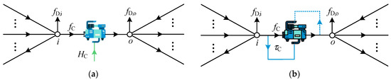
Figure 3.
Generalized structure diagrams of the compressors. (a) Compressor driven via electric motor; (b) compressor driven via gas turbine.
Compared with MCs, TCs are isolated from other subnetworks, as they are powered via gas turbines. As depicted in Figure 3b, the consumed gas flow, τC, can be extracted from both the inlet and outlet of TC [40], whose numerical value is approximated as follows:
where the following applies: τC,st is the equivalent energy consumption vector of the extracted gas under standard GCV; αC, βC and γC are the coefficient vectors of energy-conversion efficiency; and qC is the GCV vector at the extraction node.
Aside from driving types of compressors, the following commonly used operation modes are also considered: (1) Mode I: the squared boost ratio = Πo/Πi is preset; (2) Mode II: the boost squared difference = Πo − Πi is preset; (3) Mode III: the gas-flow rate is preset; (4) Mode IV: the squared inlet pressure is preset; and (5) Mode V: the squared outlet pressure is preset.
The general relationship between the inflow and outflow of gas nodes is illustrated in Figure 4. The upstream flow with significant composition differences can originate from various gas sources, pipelines, or transmission equipment. Meanwhile, the downstream flow with uniform gas concentration may be injected into gas customers, gas-driven coupling devices, pipelines, or transmission equipment. It has been revealed that models containing loop equations cannot universally describe gas energy flow when variable compressor modes are considered [40,41]. Additionally, conventional gas NPMs also fail to depict the generalized compressor connection structure [42]. Therefore, an expanded NPM originated from [43] is utilized and modified as the cornerstone of the proposed DGN model.
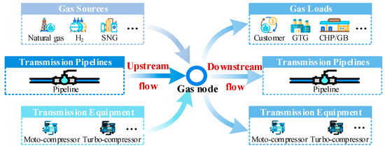
Figure 4.
Generalized schematic diagram of gas mixture process.
Analogous to Kirchhoff’s current law, the sum of the gas volume flow at each node should be zero. Thus, the nodal volume flow balance equation can be formulated as follows:
where the following applies: Bg = [ ] is the node-equipment incidence matrix; is the node-slack source incidence matrix; is the node-compressor incidence matrix; TC is the node-extraction incidence matrix; fE is the equipment gas-flow vector; fS is the slack source flow vector; fL = fD − fI is the net load flow vector; fI is the non-slack source flow vector; fD = ED · q−1 is the load volume demand vector; ED is the load energy demand vector; and q is the gas-flow GCV vector.
The following equipment control equation is constructed to characterize the diversity of equipment modes. The formulation for the k-th equipment can be written as follows:
where the following applies: is the DGN equipment set; Πs/Πi/Πo is the squared pressure of slack source node s/compressor inlet node i/compressor outlet node o; fE,k is the gas flow of the k-th equipment; and wN,ks, wN,ki, wN,ko, wE,k, and dk are the control parameters of different equipment modes, whose values are given in Table 2. Equation (24) can be further rewritten into the compact matrix form as follows:
where the following applies: WN is the coefficient matrix of squared node pressure whose nonzero elements in the k-th row and s-th/i-th/o-th column is wN,ks/wN,k/wN,ko; WE = diag(wE,k) is the coefficient matrix of equipment flow; and d is the vector of dk.
Table 2.
Values of control parameters for different equipment modes.
Finally, the gas hydraulic model is derived by combining Equations (19), (21)–(23), and (25), which is adaptable to simulate the DGN automatically, regardless of network topologies and equipment modes.
2.3.2. Gas Composition-Tracking Model
The gas composition-tracking model is essential for exposing the impact of dissimilar gas sources on the network state. According to the mass and energy conservation, the nodal mass flow and nodal energy-flow balance equations are represented in recursive form:
where the following applies: is the set of pipelines flowing into/out of node i; / is the set of compressors flowing into/out of node i; is the set of compressors extracting from node i; is the set of gas source types; is the set of DGN nodes; / is the pipeline flow entering/exiting node i; / is the compressor flow entering/exiting node i; ρin/ρout is the specific gravity of gas entering/exiting node i; qin/qout is the GCV of gas entering/exiting node i; / is the known-pressure/known-injection source flow of type ℓ; and ρℓ/qℓ is the gas specific gravity/GCV of type ℓ.
Similar to the established DHN model, incidence matrices are employed in the DGN to define the inflow and outflow relationships. The compact matrix representation of Equation (26) is obtained as follows:
where the following applies: is the node-slack source type incidence matrix; ρSource/qSource is the vector of specific gravity/GCV of different slack source types; is the node-non-slack source type incidence matrix; and is the non-slack source flow vector of type ℓ. It should be emphasized that ρ, q, and other gas property variables mentioned in this work refer to the characteristics of outflowing gas from certain nodes, which are unknown for every DGN node, even slack nodes. Moreover, multiple types of gas sources can be injected into the same node simultaneously, provided that their injection volume proportions (for slack sources) or injection flow rates (for non-slack sources) are defined.
To monitor the volatility of other physical properties, molar fractions for different gas-source types are introduced. Referring to Equation (27), the nodal molar fraction for type ℓ is also derived in matrix form:
where εℓ is the molar fraction vector of gas type ℓ, and is the column of associated with gas type ℓ.
The gas is often assumed to behave ideally according to the ideal gas law in previous studies. It holds naturally for low-pressure conditions. However, as gas pressure increases, the discrepancy between real and ideal gas behavior cannot be ignored. Therefore, the real gas equation of state (EoS) is applied to the gas mixture process:
where pg/ρg/Zg/R is the pressure/density/compressibility factor/gas constant of the mixture. Several virial-type models for calculating Zg have been derived based on experimental measurements, each suited to different application scenarios. Herein, the empirical model of the American Gas Association (AGA) [39] that is applicable for pressure up to 70 bar is adopted to update ZP in Equation (20), and its matrix formulation is given as follows:
where the following applies: is the average pressure of the mixture; ps/pe is the pressure vector of the pipeline start/end node; and Tcr/pcr is the critical temperature/pressure vector of the mixture, which can be estimated using Kay’s mixing rule:
where υ denotes the vector of certain property of the mixture; υℓ denotes the certain property of gas type ℓ. Analogously, ZC,in and ω in Equation (21) can also be revised by the following equation:
where ωcp/ωcv is the specific heat capacity vector at constant pressure/volume for the mixture, whose value is also calculated by Equation (31). Accordingly, based on the proposed gas composition-tracking model comprising Equations (27), (28), and (30)–(32), the impact of alternative injections on gas flow can be quantified accurately.
2.4. Energy-Conversion Device Formulation
CHP units with back-pressure turbine (CHPI) and extraction-condensing turbine (CHPII) are given by Equations (33) and (34), respectively:
where qgas is the gas GCV; Φx/Px/fx is the heat power/electrical power/gas consumption of device x; ηx is the electrical or heat efficiency of device x; zCHPI is the heat-to-power ratio of CHPI; zCHPII is the ratio quantifying the increase in heat power and the decrease in electrical power of CHPII.
The models of GTG and GB are formulated as follows:
The output power of HP/EB is written as follows:
Considering the potential safety risk of blending large amounts of hydrogen directly into the DGN [37], P2G is targeted to produce SNG, whose mathematical formula is as follows:
where the following applies: fP2G and PP2G are the injected SNG flow rate and the consumed power of P2G; ηP2G is the energy-conversion efficiency; and qSNG is the GCV of SNG.
The required power of MCs and circulation pumps (CPs), PC and PCP, are written as follows:
where mcp is the mass flow through the pump, g is the gravitational acceleration, and hcp is the pump head.
Aside from the above coupling devices, this work also considers traditional standalone devices, including independent sources and energy storage devices for each subsystem, with their formulations detailed in [22].
3. Iterative Matrix Derivation of IEHGES
Considering the high-dimensional and nonlinear properties of multi-energy-flow equations, the well-known NR technology is adopted for the EFC solution. As the iterative matrix (Jacobian matrix) significantly affects the convergence of the model solution, the derivations of iterative matrices for the proposed model are performed in this section.
3.1. Derivation of the Iterative Matrix for DEN
The electric mismatch vector Fe is given as follows:
where ΔP/ΔQ represents the mismatch equations of active/reactive power. The state variable vector in Equation (40) is xe = [θ; |V|], where θ/|V| is the voltage angle/magnitude vector. Thus, the iterative matrix of DEN Jee can be represented as the partial derivatives of Fe with respect to the unknown state variables:
The detailed formulation of Jee can be referenced in [12].
3.2. Derivation of the Iterative Matrix for DHN
By combining the proposed DHN hydraulic and thermal models, the heat mismatch vector Fh is obtained via the following:
Note that the mismatch equations of hTs node are excluded from ΔΦs; Δhf should be eliminated if the DHN topology is radial. Similar to [15], the state variable vector in Equation (42) is xh = [m; ′; ′]. Hence, the iterative matrix for the DHN Jhh is described as follows:
Since no modifications have been made to the hydraulic model, the expressions for submatrices in the first row of Jhh follow [15]. For the rest, ∂Δ′/∂′ and ∂Δ′/∂′ are typically constructed through traversal. Instead of using this inefficient approach, the formulations of these two partial derivatives are revised as follows:
In terms of ∂Δ′/∂m and ∂Δ′/∂m, most existing research approximates their elements to zero for simplicity. However, this approximation will deteriorate the convergence of the iterative EFC process, particularly when the absolute values of their elements are not much smaller than the corresponding diagonal elements in Jhh [23]. Therefore, the matrix-based formulations for these two partial derivatives are derived as follows:
3.3. Derivation of the Iterative Matrix for DGN
The gas mismatch vector Fg can be easily expressed from its mathematical model:
Let the unknown state variable vector in Equation (46) be xg = [Π; fE; ρ; q], and the iterative matrix of DGN Jgg can be expressed as follows:
Similarly, a few elements of Jgg are also neglected in the previous research [28], causing the non-gradient-descent direction of the NR iteration. To handle this issue, the matrix formulation of each submatrix in Jgg is derived as follows:
On this basis, the iterative matrices with a gradient-descent direction for each subnetwork of IEHGES can be obtained via matrix operations.
4. EFC Solution Method
To address the complicated coupling relationships between subnetworks, a thorough discussion of the interdependency mechanism within IEHGES is presented, based on which the NR-based integrated and decomposed EFC methods (NRIM and NRDM) are developed in this section.
4.1. Coupling Chain of the Device
Coupling devices facilitate energy interactions between individual subnetworks. Therefore, to investigate the interdependency mechanism within IEHGES, the attributes of coupling devices are classified in Table 3.
Table 3.
Attribute classification of coupling devices.
As described in Table 3, a single device can serve as the slack units of multiple subnetworks, whereby defining its category. The node types of device ports and the coupling relationships established by devices are all reflected in device categories. For instance, if a CHP works in FEL mode, its category will be ‘ES’, and its coupling chain will be ‘G←E→H’, indicating that the operating states of the DGN and DHN depend on that of the DEN. For another example, an MC categorized as ‘NS’ may either be shut down or powered via an independent electric source, wherein no coupling chain or node type is present. Note that all the coupling chains are directional. The initiator of the arrow is the dominator of this coupling chain, influencing the state of the terminal of the arrow. Additionally, the coupling chains can be superimposed under certain constraints, creating more complicated interdependencies.
4.2. Interdependency Mechanism Analysis
Generally, each subnetwork has one slack unit. Following this assumption, coupling devices with varying numbers, types, and categories can be utilized to interconnect each subnetwork, leading to numerous possible combinations of devices. Although the physical connection schemes within IEHGES are innumerable, the potential combinations of superimposable coupling chains remain finite, which is generalized in Figure 5. In Figure 5, the DGN dominates the DEN via MC/P2G, the DHN influences the DGN and DEN via GB/CHP and EB/HP/CHP/CP, respectively, while the DEN regulates the DHN and DGN via CHP and GTG/CHP, respectively.
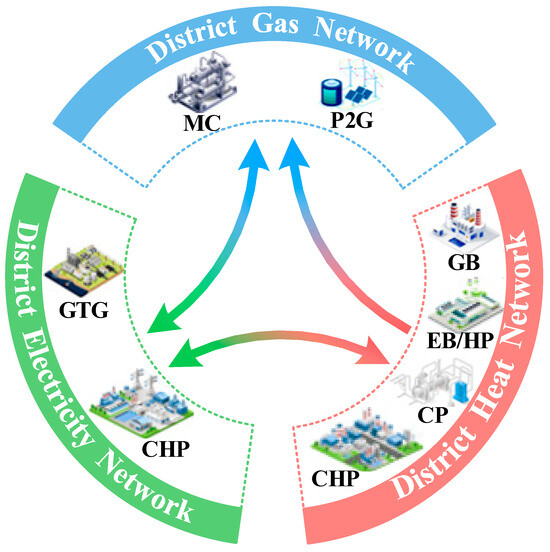
Figure 5.
Generalized schematic of coupling chains within IEHGES.
The generalized interdependency mechanism of IEHGES is further concreted into different coupling modes, as illustrated in Figure 6. According to the numbers and types of closed loops formed by coupling chains, four coupling modes are identified from the limited combination possibilities of coupling chains, which are described as follows:
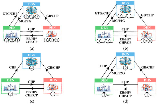
Figure 6.
Interdependencies of IEHGES under different coupling modes. (a) Mode 1.1/1.2/1.3; (b) Mode 2.1/2.2; (c) Mode 3; (d) Mode 4.
- Mode 1: Subnetworks are unidirectionally coupled or decoupled with each other;
- Mode 2: Mutual coupling exists merely between DEN and DGN;
- Mode 3: Mutual coupling exists merely between DEN and DHN;
- Mode 4: Mutual couplings exist simultaneously between DEN and DGN, and between DEN and DHN.
Specifically, mode 1 contains three scenarios: (1) the slack unit of DEN is an independent source, namely mode 1.1; (2) GTG belongs to ‘ES’, while MC and P2G belong to ‘NS’, namely mode 1.2; and (3) CHP works as ‘ES’, while MC, P2G, EB, HP, CHP, and CP work as ‘NS’, namely mode 1.3.
Mode 2 is determined when IEHGES satisfies one of the following two conditions: (1) GTG belongs to ‘ES’, while MC or P2G belongs to ‘GS’, namely mode 2.1; (2) CHP works as ‘ES’, MC, or P2G works as ‘GS’, while GB, EB, HP, CHP, and CP work as ‘NS’, namely mode 2.2.
Scenarios become unitary for modes 3 and 4. In mode 3, CHP works as ‘ES’, and MC and P2G work as ‘NS’, while EB, HP, CHP, or CP works as ‘HS’. In mode 4, CHP belongs to ‘ES’ or MC, and P2G belongs to ‘GS’, while GB, EB, HP, CHP, or CP belongs to ‘HS’.
On this basis, the interdependency category of IEHGES can be automatically recognized via Algorithm 1. The solution procedure for each coupling mode is identical in NRIM but quite different in NRDM. In modes 1.1–1.3, the EFC solution is implemented once for each subnetwork in three distinct sequences. The specific solution orders are determined according to the directions of coupling chains, as shown in Figure 6a, which are DHN→DGN→DEN, DHN→DEN→DGN, and DEN→DHN→DGN, respectively. Things get more complicated in modes 2–4 due to mutual effects. Mode 2–4 are related to four different solution processes in NRDM, with the specific solution sequences indicated in Figure 6b–d, which can be illustrated as DHN→DGN↔DEN for mode 2.1, DGN↔DEN→DHN for mode 2.2, DHN↔DEN→DGN for mode 3, and DHN→DGN→DEN→… for mode 4. Taking mode 3 as an instance, the energy flow of the DHN is solved first with an assumed heat power of the CHP working as ‘ES’. Subsequently, the energy flow of DEN is determined using the calculated electric power of the CHP working as ‘HS’. The EFC calculations of these two mutually coupled subnetworks are iteratively performed until the convergence is achieved. After that, the DGN model can be directly solved to finalize the EFC results of IEHGES.
| Algorithm 1: Coupling mode determination. | ||||
| 1 | Initialization: Input parameters of the coupling devices | |||
| 2 | if GTG & CHP belong to ‘NS’ then | |||
| 3 | Coupled in mode 1.1; break | |||
| 4 | else | |||
| 5 | if GTG belongs to ‘ES’ then | |||
| 6 | if MC & P2G belong to ‘NS’ then | |||
| 7 | Coupled in mode 1.2; break | |||
| 8 | else | |||
| 9 | Coupled in mode 2.1; break | |||
| 10 | else | |||
| 11 | if MC & P2G belong to ‘NS’ then | |||
| 12 | if EB & HP & CHP & CP belong to ‘NS’ then | |||
| 13 | Coupled in mode 1.3; break | |||
| 14 | else | |||
| 15 | Coupled in mode 3; break | |||
| 16 | else | |||
| 17 | if GB & EB & HP & CHP & CP belong to ‘NS’ then | |||
| 18 | Coupled in mode 2.2; break | |||
| 19 | else | |||
| 20 | Coupled in mode 4; break | |||
| 21 | end if | |||
| 22 | end if | |||
| 23 | end if | |||
| 24 | end if | |||
| 25 | Output the coupling mode of the IEHGES. | |||
4.3. NR-Based Solution Strategy
The general iteration form of the NR method is given as follows:
where the following applies: λ is the damping factor, which is usually default as 1; x is the unknown variable vector; F is the mismatch vector; k is the iteration index; and J is the iterative matrix.
For NRIM, the state variables is x = [xe; xh; xg], the mismatch equations is F = [Fe; Fh; Fg], and J is formulated as follows:
The iterative matrix J consists of two parts. The formulations for diagonal block matrices Jee, Jhh, and Jgg have been derived in Section 3. For the remaining part, xy denotes the effect of subnetwork y to subnetwork x, whose formulation depends not only on the coupling device model but also on the category and node type of the device [25]. The dimension of J equals the number of state variables, which is (Ne + Npq – 1) + (Nhp + 2Nhn) + (3Ng + Nge). Npq/Nhp/Nhn/Ng/Nge is the number of PQ buses/heat pipelines/heat non-source nodes/gas nodes/gas equipment. Algorithm 2 outlines the detailed EFC solution procedures for NRIM. The solution starts from the system parameter initialization and elementary incidence matrix generation. Then, based on the proposed numerical model, the NR iteration and intermediate variable update are executed continuously until either the maximum value of |F| falls below ζ or the iteration number exceeds K.
| Algorithm 2: NR-based integrated method (NRIM) | ||
| 1 | Initialization: Input convergence tolerance ζ, maximum iteration number K, initial value of x = [θ; |V|; m; ′; ′; Π; fE; ρ; q], parameters of networks and coupling devices; the iteration index k = 0. | |
| 2 | Compute the elementary incidence matrices. | |
| 3 | while k ≤ K do | |
| 4 | Compute mismatch vector Fk according to Equations (40), (42) and (45). | |
| 5 | if max(|Fk|) ≤ ζ then | |
| 6 | break | |
| 7 | end if | |
| 8 | Compute iterative matrix Jk according to Equation (63). | |
| 9 | Update xk+1 according to Equation (62). | |
| 10 | Update Ahd and Agd according to Equations (8) and (20). | |
| 11 | Update mq, ′ and ′ according to Equations (3), (14) and (17). | |
| 12 | Update ε, ZP, ZC,in and θC according to Equations (28), (30)–(32). | |
| 13 | Update fP, HC, and τC according to Equations (19)–(22). | |
| 14 | Update k = k + 1. | |
| 15 | end while | |
| 16 | Output the energy-flow results of the IEHGES. | |
Compared with NRIM, NR calculation is individually applied to each subnetwork for NRDM. The specific EFC process for each subnetwork can be obtained by excluding other subnetworks from Algorithm 2. Subsequently, NRDM is implemented by performing the EFC solution for each subnetwork in particular orders described in Section 4.2.
In summary, a matrix-based universal framework for the steady-state analysis of IEHGES has been established, which achieves the standardized modeling and solution of multi-energy flow. The flow chart of the framework is presented in Figure 7, and the main steps are as follows:
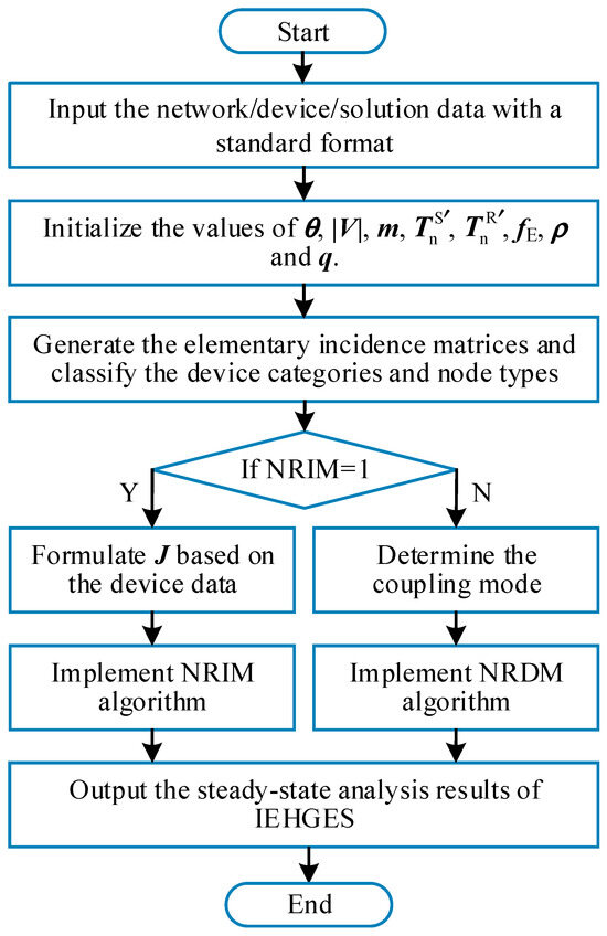
Figure 7.
Flowchart of the proposed matrix-based universal EFC framework.
- Step 1: Input the system data in a standard format [44], including the network data, device data, and solution algorithm data;
- Step 2: Initialize the values of state variables θ, |V|, m, ′, ′, Π fE, ρ, and q. In this work, the commonly adopted initialization method in [31] is employed;
- Step 3: Generate the elementary incidence matrices Ah, Bh, Ag, Bg, W, and TC according to the input data. Classify the categories and node types of the coupling devices according to Table 2;
- Step 4: Execute the corresponding algorithm according to the solution instruction. If NRIM is selected, formulate the expression of J based on the device data, and then implement Algorithm 2; if NRDM is chosen, determine the coupling mode by implementing Algorithm 1 and then implement the corresponding NRDM algorithm;
- Step 5: Output the steady-state analysis results of IEHGES.
5. Case Studies
To validate the performance of the proposed framework, a medium test system comprising the IEEE 30-bus DEN [45], 32-node Barry Island DHN [15], 14-node DGN [40], and several coupling devices is established, and its schematic is shown in Figure 8. The CHP, GB, and natural gas well serve as the slackers of DEN, DHN, and DGN, respectively. Circulation pumps at nodes H1, H31, and H32 are driven via buses E8, E2, and E5. Compressors 1 and 4 are powered via buses E15 and E20, while the remaining compressors are TCs extracting from the inlet nodes. Compressors 1–4 all work in mode I. Hydrogen storage, SNG storage, and P2G constitute the distributed gas sources. Accordingly, the described system is judged to be operating in the most complex mode, i.e., mode 4.
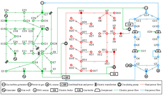
Figure 8.
Structure schematic of the medium test system.
The detailed parameters of the subnetworks and coupling devices are provided in [44]. The convergence and iteration tolerances for NR calculation are 10−8 and 100 times, respectively. The DEN and DHN are initialized at |V| = 1 p.u., θ = 0°, m = 100 kg/s, ′ = 100 °C and ′ = 30 °C, while a pressure difference of 5–10% between the receiving and sending node is considered for initializing p. fE is then calculated from p. The gas property values of the natural gas are adopted to initialize ρ and q, which are 0.610 6 and 41.04 MJ/m3, respectively. Gas temperature is fixed at 288.15 K, and STP is defined as 293.15 K and 1.013 25 bar. Other characteristic parameters of heterogeneous gas sources are listed in Table 4. Simulations in this section are solved by MATLAB 2023a on a laptop with Intel(R) Core(TM) i9-13900H CPU @2.60GHz and 16.0 GB memory.
Table 4.
Property of different types of gas sources [46].
5.1. Accuracy Analysis
Due to the lack of a control group, the effectiveness of the proposed gas composition-tracking model is first verified through quantitative analysis. The gas property results of the proposed matrix-based models (PM) solved via NRIM and NRDM are depicted in Table 5 and Table 6. It can be observed that both NRIM and NRDM yield identical results, further validated by calculations from Equations (30)–(32) and (46). Unlike conventional DGN models with constant gas characteristics, multiple gas properties vary across the network, demonstrating the gas composition-tracking capability of PM. As illustrated in Table 5, specific gravity and GCV are closer to discrete variables compared with the continuously varying pressure, as their values merely depend on the gas molar fraction. Table 6 shows that compressors 1 and 3, as well as 2 and 4, have the same polytropic coefficients since the gas compositions are identical at their inlet ends, which is consistent with Equation (32). Conversely, the gas-compressibility factors for pipelines and compressors differ from each other. The main reason is that they are affected not only by the gas molar fraction but also by pipeline pressure, as indicated in Equations (30) and (32).
Table 5.
Nodal pressure, specific gravity, and GCV in the medium test system.
Table 6.
Compressibility factor and polytropic coefficient in the medium test system.
After that, the traditional EFC models (TM) for DHN [15] and DGN [28], whose mismatch vectors and iterative matrices are formulated in recursive form, are built for comparison. The proposed gas composition-tracking model is also added in TM but programmed recursively. Since no modification has been made for DEN, the modeling of DEN in PM and TM refers to [12]. PM and TM are tested on the medium test system, and the corresponding absolute errors of EFC results between PM and TM are given in Table 7. As depicted in Table 7, the maximum absolute errors in NRIM and NRDM are 1.94 × 10⁻⁹ MJ/m3 and 1.89 × 10⁻⁹ MJ/m3, respectively, which are less than 10−8, indicating the accuracy of PM. In summary, the proposed framework is capable of characterizing the energy-flow distribution of IEHGES while precisely tracking the gas composition.
Table 7.
The EFC errors between PM and TM for the medium test system.
5.2. Universality Analysis
In this subsection, the proposed framework is applied to various IEHGES operation scenarios to demonstrate its universality. All the designed scenarios below are generated by revising the input files of the benchmark scenario, i.e., the original medium test system.
5.2.1. Diversity of Heat Sources
In the benchmark scenario, loads at heat nodes H7 and H17 are replaced with two thermal storage devices to represent the diversity of heat sources. The charging/discharging power of thermal storage equals the original nodal load power. To manifest the applicability of PM across different heat sources, the following two scenarios are considered:
- Scenario 1: The thermal storage is discharging at H7 but charging at H17.
- Scenario 2: The thermal storage is discharging at H17 but charging at H7.
The heat energy flow of Scenario 1 is modeled through PM and TM, with their supply temperature results in Figure 9a. A notable deviation in supply temperature is observed between TM and PM around H7. This discrepancy arises because TM incorrectly defaults the supply temperature at H7 to , whereas H7 is actually a mixing node. This miscalculation of DHN propagates through other subnetworks along the coupling chains, ultimately leading to an inaccurate assessment of the IEHGES operation status. Furthermore, other DHN formulations in [18,19,20,21,22] encounter similar issues, as they lack nodal temperature equations for source nodes.
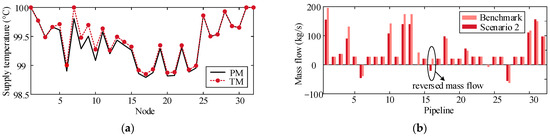
Figure 9.
The EFC results of DHN in benchmark and Scenario 1 and 2. (a) Supply temperature of DHN solved by PM and TM in Scenario 1; (b) mass flow of DHN in benchmark and Scenario 2.
Once the discharging thermal storage transfers from H7 to H17 in Scenario 2, PM remains effective in characterizing the energy flow distribution, whereas TM fails to converge as reported in [22]. The mass flow results for both the benchmark scenario and Scenario 2 are shown in Figure 9b. It is observed that the mass flow in pipeline 16 reverses from 20.97 kg/m3 to −20.56 kg/m3 due to the state switching of the thermal storage. Since existing DHN models do not account for the generalized heat energy-flow direction, they are more sensitive to inappropriate hydraulic initialization, resulting in their failure in Scenario 2.
5.2.2. Diversity of Gas Properties Considered in DGN
Although PM is established towards heterogeneous gas-source mixing, it is versatile enough to be applied in various scenarios where different categories of gas properties are considered:
- Scenario 3: Based on the benchmark, part of the gas properties are treated as constants by setting ZP, ZC,in, and ω to 0.8, 0.8, and 1.309 [25], respectively.
- Scenario 4: Based on Scenario 3, only natural gas sources are injected into the DGN. It is achieved by setting ρ and q to constants 0.610 6 and 41.04 MJ/m3, respectively, while the injection amount of alternative gas sources is adjusted to be energy-equivalent to that in other scenarios.
Note that gas loads in different scenarios are also energy-equivalent in this subsection. Table 8 and Table 9 and Figure 10 display the EFC results of different scenarios solved through PM.
Table 8.
Nodal pressure of DGN in Scenarios 3 and 4.
Table 9.
The interdependencies of benchmark and Scenario 3 and 4.
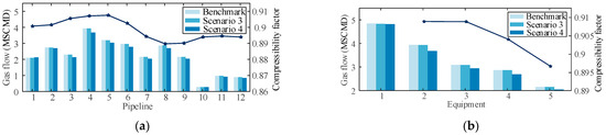
Figure 10.
The EFC results of DGN in benchmark and Scenario 3 and 4. (a) Pipeline gas flow and compressibility factor of DGN; (b) equipment gas flow and compressibility factor of DGN.
As depicted in Table 8, the nodal pressures in Scenarios 3 and 4 differ from the benchmark due to the consideration of various gas properties. Gas flow in the DGN is primarily affected by load demand. A reduced GCV, combined with a constant load energy demand, increases gas flow. According to the gas pipeline equation = ΔΠ/(Cpipeρ), although the gas density ρ decreases, the pressure drop, ΔΠ, increases because of the rising gas flow, fP, and the fixed pipeline parameter, Cpipe. This explains why the nodal pressure in Scenario 3 is lower than that in Scenario 4. Furthermore, according to Table 6, the pipeline compressibility factors in the benchmark scenario are greater than those in Scenario 3. As defined in the gas pipeline equation, this difference further facilitates the pressure drop in the benchmark. Analyzing the pressure differences between Scenario 3/4 and the benchmark in Table 8 reveals that the pressure deviations caused by each pipeline accumulate along the gas-flow direction, eventually reaching a maxima value at node G14. In terms of gas flow, Figure 10 illustrates that Scenario 4 has the lowest flow rate due to its highest GCV. The gas flow of Scenario 3 is similar to that of the benchmark since their load energy demands and GCVs are comparable. Per Equation (21), the higher the compressor flow or compressibility factor, the larger the energy consumption of the compressor. This is why PC and τC in Table 9 show a descending trend from the benchmark to Scenario 3 and then to Scenario 4. The energy-flow discrepancies in the DGN across different scenarios propagate to the DEN through MCs, causing fluctuations in the output of CHP, which subsequently alters the output of GB. Consequently, the operation states of the DEN and DHN also vary in different scenarios due to the interdependencies within IEHGES.
In brief, PM has been proven to be scalable for various application scenarios. Unlike traditional DGN models, PM avoids inaccurate estimations of nodal gas pressure by comprehensively considering the impacts of physical characteristics on gas-flow distribution. This capability is crucial for developing rational gas-network scheduling strategies and safeguarding the gas supply quality of downstream customers.
5.2.3. Diversity of Compressor Operating and Driving Modes
To further illustrate the universality of PM, scenarios featuring various operating and driving modes of compressors are designed:
- Scenario 5: Compressors 1–4 are replaced with TCs from the benchmark, operating in modes II, I, III, and V, respectively.
- Scenario 6: Compressors 1–4 are replaced with MCs from the benchmark, operating in modes I, III, II, and IV, respectively.
Figure 11 represents the EFC results of each subnetwork in different scenarios. As shown in Figure 11a, the gas pressures of Scenarios 5 and 6 are overall lower and higher than those of the benchmark, respectively, due to the different operation modes and control parameters of compressors. The number of MCs driven via the DEN in benchmark, Scenario 5, and Scenario 6 are 2, 0, and 4, respectively. Consequently, the voltage angles in the benchmark lag behind those in Scenario 5 but lead those in Scenario 6, as depicted in Figure 11b. According to the varying mass flow of DHN given in Figure 11c, this influence on DEN is further extended to DHN. Therefore, it can be deduced that the universality of the IEHGES energy-flow analysis method for diverse compressors is necessary.
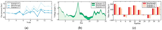
Figure 11.
The EFC results of IEHGES in benchmark and Scenario 5 and 6. (a) Nodal pressure of DGN; (b) voltage angle of DEN; (c) mass flow of DHN.
5.3. Robustness Analysis
The convergence performance of PM is compared with that of TM by adjusting the initial values (including |V|, m, p, and the initial guess ΦCHP in NRDM) and load levels of the benchmark through scaling factors, thereby validating the robustness of the proposed framework.
5.3.1. Effectiveness with Different Initializations
The distinction in iterations between PM and TM under different initializations is summarized in Table 10. As can be seen, TM solved by NRIM converges only with default initial values, whereas PM exhibits a broader convergence range of 80–160% of the original initialization. This difference arises because improper initializations, such as excessively high or low values of |V|, or inappropriately initialized p, may result in the negative output of the slack CHP during the iteration, which reverses the heat source of DHN simultaneously, eventually facilitating the singular Jacobian matrix of TM. The same problem occurs in other DHN models [18,19,20,21,22]. Since the bidirectional DHN model is established, this defect can be overcome in PM. Moreover, by comparing the convergence curves of different subnetworks under the original initialization in Figure 12, it can be found that each subnetwork in PM satisfies the mismatch tolerance of 10−8 within 10 steps. In contrast, the DHN and DGN in TM require 23 and 32 iterations to converge, respectively. This is because ∂Δ′/∂m and ∂Δ′/∂m of Jhh, ∂Δρ/∂q and ∂Δq/∂ρ of Jgg are both omitted in TM. Thus, the non-gradient-descent direction of the iterative matrix in TM causes a slower reduction in mismatches, further reflecting the correctness of the iterative matrix derivation for PM.
Table 10.
Comparison of iterations under different initializations.
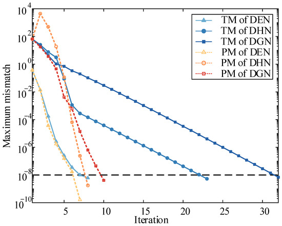
Figure 12.
Iteration process of each subnetwork under original initialization.
The convergence of PM and TM are also tested through NRDM, as shown in Table 10. Similarly, the excessively high value of ΦCHP can also cause the reversed mass flow of the heat source so that TM fails to converge. In contrast, owing to its iterative matrix with a gradient-descent direction, PM converges successfully for each scaling factor with fewer average inner-layer iterations.
5.3.2. Effectiveness with Different Initializations
All kinds of loads in the benchmark are varied with the scaling factor, and the corresponding iteration results of PM and TM are presented in Table 11. It is observed that the iteration number of TM increases with rising load levels until the scaling factor exceeds 120%, whereas PM effectively operates across all load levels with a faster convergence rate. However, as the scaling factor increases, the mass flow of heat slack source GB may decrease and even reverse as the increment in ΦCHP surpasses that of the heat loads. Hence, although PM converges to scaling factors greater than 120%, the values of ΦGB turn negative, which is not allowable under real-world conditions. This indicates that PM is applicable not only for normal operation states but also for some extreme impermissible scenarios, thereby helping avoid potential operation risks of IEHGES.
Table 11.
Comparison of iterations under different load levels.
Additionally, the convergence performance of PM in DHNs containing small communities with light loads is also a critical indicator of its robustness [23]. Herein, three types of models, including PM, TM, and PM without ∂Δ′/∂m and ∂Δ′/∂m in Jhh, are tested by reducing the heat load at H10 based on the benchmark. The simulation results solved via NRIM are depicted in Figure 13. PM successfully converges after 10 steps, while oscillations appear in the iteration processes of other models. Figure 14 presents the partial heatmap of |Jhh| calculated through PM in the final iteration. The reduction in load H10 causes a significant decrease in the diagonal element of the correlative row of Jhh. In this circumstance, only the accurate calculation of ∂Δ′/∂m ensures the iteration progresses in the correct direction, highlighting PM’s superior robustness under light load conditions.
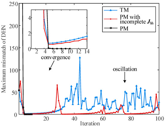
Figure 13.
Iteration process of energy-flow model with light heat load.
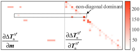
Figure 14.
Partial heatmap of |Jhh| for DHN with light load.
5.4. Efficiency Analysis
To demonstrate the superiority of PM in computational efficiency, the average execution time of PM and TM across various coupling modes and solution methods is compared in Table 12. The IEHGESs coupled in modes 1–3 are obtained by modifying system parameters from the benchmark:
Table 12.
Comparison of computation time under different coupling modes.
- Mode 1: MCs and CPs are powered independently.
- Mode 2: CPs and GB are powered independently.
- Mode 3: MCs are powered independently.
Note that the neglected elements in the iterative matrix of TM are supplemented in recursive form to prevent discrepancies in computational efficiency caused by iteration numbers.
The efficiency-gain ratio is defined as the multiple of TM consumption time relative to PM consumption time. The shorter the calculation time of PM, the greater the gain ratio, and the higher the efficiency of PM. As shown in Table 12, the computation efficiency of PM is consistently higher than that of TM in each coupling mode, even though both models utilize iterative matrices with gradient-descent direction in this test. Specifically, the execution time of NRIM remains unaffected by the coupling mode since the energy-flow distributions and iteration numbers are similar in modes 1–4, maintaining a gain ratio of PM to TM at around 1.6. Conversely, the time consumption of NRDM fluctuates across modes 1–4 due to the use of different solution sequences. As the degree of interdependency deepens, the efficiency of NRDM decreases while the gain ratio of PM to TM rises from 1.718 7 to 1.994 0. This is because more subnetworks are involved in the inner-layer iteration as the coupling effect strengthens. It should be remarked that no code optimization or additional acceleration algorithms are applied in this test. Compared with the recursive loops used in TM, PM has the potential of fully utilizing the hardware capabilities and optimization techniques of modern computers owing to its matrix-based structure [13], reducing efficiency losses caused by repeated updating of mismatch equations and the Jacobian matrix in NR-based methods.
5.5. Large-Scale Capability
To further validate the effectiveness of the proposed framework, a larger test system consisting of IEEE 118-bus DEN [45], 51-node DHN in Jilin Province [20] and 48-node DGN [31] with 8 compressors operating in mode I, is established, and its schematic is shown in Figure 15. The system parameters provided in [44] are set as the benchmark scenario of this larger-scale system, where CHPI, CHPII, and P2G, as well as two natural gas wells, serve as the slackers of DEN, DHN, and DGN, respectively.
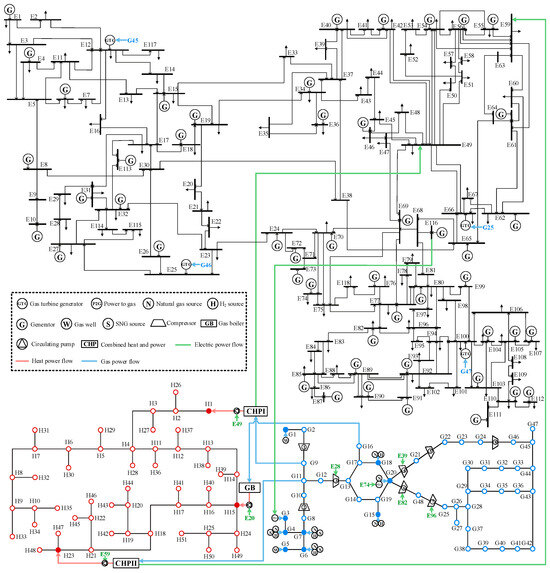
Figure 15.
Structure schematic of the large test system.
5.5.1. Effect of Compressibility Factor on Energy-Flow Analysis
Given that the variation in the compressibility factor is commonly ignored in previous studies, Scenarios 7–9 and the benchmark scenario of the large system are adopted for investigating the impact of compressibility factor on EFC, whereby demonstrating the suitability of PM on large-scale IEHGES. Specifically, all gas properties in the benchmark scenario are determined using the proposed gas composition-tracking model. Based on the benchmark, Scenarios 7–9 set ZP/ZC,in to 0.8, the average value in the benchmark scenario, and 1, respectively, and set ω to 1.309. The comparisons of EFC results under different scenarios are shown in Figure 16.
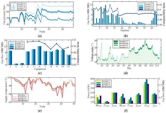
Figure 16.
The EFC results of IEHGES in benchmark and Scenario 7–9. (a) Nodal pressure of DGN; (b) pipeline gas flow and compressibility factor of DGN; (c) equipment gas flow and compressibility factor of DGN; (d) voltage angle of DEN; (e) supply temperature of DHN; (f) interdependencies of IEHGES.
As illustrated in Figure 16a–c, the nodal pressure differs markedly among scenarios, while the gas flow remains relatively constant. In Scenarios 7 and 9, compressibility factors that are either too low or too high result in the overestimation and underestimation of nodal pressure relative to the benchmark, respectively, which is particularly pronounced in the downstream region of the DGN. Compared with the medium system, the pressure deviations here are more severe. This is not only due to the greater accumulation of pressure errors but also because compressors operating in mode I exhibit a more pronounced bias amplification effect. In contrast, the state deviation of the DGN in Scenario 8 is considerably smaller compared to Scenarios 7 and 9 since the compressibility factors of the benchmark and Scenario 8 are similar. However, according to Figure 16d–f, the interdependencies of the IEHGES, as well as the states of the DEN and DHN, vary noticeably from the benchmark in Scenarios 7–9, regardless of the state deviation degree of the DGN. The main reason is that even a slight variation in gas production can be converted into a more substantial energy difference through P2G, ultimately leading to different operation states of the IEHGES in each scenario. Additionally, since the power consumption of P2G is bigger than that of MC, the energy-flow deviations in the large IEHGES are greater than that of the medium system. Hence, it can be deduced that a precise compressibility factor is necessary for the accurate EFC of DGN and even the whole IEHGES, especially when the energy interaction between the DGN and other subnetworks is considerable.
5.5.2. Computational Efficiency for Large-Scale System
Additionally, the computational efficiency of PM for the large-scale system is also verified in the same manner as in Section 5.4. Different system-coupling modes are accomplished by adjusting the driving or operating modes of coupling devices. The comparison of computational efficiency under each coupling mode is shown in Table 13.
Table 13.
Comparison of computation times under different coupling modes.
As described in Table 13, despite the increase in the running time of both PM and TM as the system scale expands, PM can still achieve better computational efficiency in every coupling mode and solution strategy. The time consumption of NRIM is relatively stable, and its average value is around 0.32 s, while the efficiency of NRDM varies obviously with the coupling modes, indicating the necessity of choosing appropriate EFC strategies for specific operating conditions. Furthermore, the efficiency gain ratios here are all higher than the corresponding values in Table 12, and the highest one reaches 2.278 6. It can be inferred that the proposed matrix structure also has advantages when dealing with large systems, not to mention the efficiency improvement potential of PM created using acceleration techniques.
6. Conclusions
This paper has proposed a universal EFC framework for fast static analysis of IEHGES, which is a systematic revision and reformulation of the classic NR-based EFC framework. By adopting a compact matrix form, the standardized modeling of energy-flow models and iterative matrices is achieved. Compared to the previous investigations on the interdependency mechanism of IEHGES, a more penetrating analysis method based on the superimposable coupling chains has been raised. On this basis, detailed EFC results of any IEHGES can be obtained from the proposed framework by inputting system parameters in a specific data format, which is fast and convenient to employ.
The effectiveness of the proposed framework was verified using two test systems of different scales. Through quantitative comparison and qualitative analysis, the established compact energy-flow model was proven to be accurate with an error of less than the convergence tolerance, i.e., 1 × 10⁻⁸. Following the generalized heat energy-flow direction, the proposed heat network model is universal to arbitrary DHNs, and its convergence is inherently improved since the RMF problem is fundamentally resolved. The simulation results under various scenarios demonstrate the applicability of the constructed novel gas-network model to diverse components of DGN. It also reflects the impact of multiple varying gas properties on energy-flow analysis, which cannot be ignored in the planning and operation of IEHGES. The robustness of the proposed framework is promoted owing to the precise iterative matrices with gradient-descent direction. Furthermore, the interdependency of IEHGES can be comprehensively categorized into four types of coupling modes. Across coupling types, more coupling chains indicate a deeper coupling degree; within the same type, greater interaction energy indicates a higher coupling degree. Finally, the efficiency gain ratios are all greater than 1.5 for two test systems, proving that the proposed matrix-based formulation has advantages in computational efficiency under each coupling mode and solution strategy. As the highest and lowest gain ratios increase from 1.99 to 2.28 and from 1.6 to 1.69, respectively, it can be concluded that this advantage becomes more pronounced with an increasing system scale and iteration numbers.
The efficiency enhancement of the proposed framework is achieved primarily at the model formulation level. Considering the potential for improvement in the temporal and spatial efficiency of matrix operation, programming schemes that leverage accelerating technologies, such as parallel computing, sparse storage, algorithm optimization, etc., should be developed in future research. Additionally, despite some minor modifications, the convergence nature of the proposed framework is largely inherited from the conventional framework. Therefore, strengthening the convergence of the proposed framework from the perspective of the solution algorithm to enhance its practical applicability constitutes another challenge for future work.
Author Contributions
Conceptualization, methodology, and writing—original draft preparation, J.W.; writing—review and editing, J.Z.; resources, F.M.; investigation, S.W., R.X. and K.L.; software, S.W. All authors have read and agreed to the published version of the manuscript.
Funding
This work was supported by the Key Research and Development Program of Jiangsu Province (Grant No. BE2020027), the National Key Research and Development Program of China (Grant No. 2022YFE0140600), and the China Scholarship Council (Grant No. 202306090135).
Institutional Review Board Statement
Not applicable.
Informed Consent Statement
Not applicable.
Data Availability Statement
The original contributions presented in the study are included in the article; further inquiries can be directed to the corresponding author.
Acknowledgments
We extend our deepest gratitude to all authors who participated in this study and contributed to the manuscript. Each author’s expertise and tireless work have been pivotal to the completion of our research findings. We wish to express our heartfelt thanks to Southeast University for the invaluable support provided in conducting the experiments of this study. The resources and facilities offered by the university have been crucial for the completion of our experimental and analytical work. Additionally, we thank the LASAR Laboratory for helpful discussions and suggestions.
Conflicts of Interest
The authors declare no conflicts of interest.
Abbreviations
The following abbreviations are used in this manuscript:
| IEHGES | Integrated electricity–heat–gas energy system |
| EFC | Energy-flow calculation |
| EH | Energy hub |
| DEN | District electricity network |
| DHN | District heat network |
| DGN | District gas network |
| AC | Alternating current |
| AE | Algebraic equation |
| HE | Holomorphic embedded |
| NR | Newton–Raphson |
| BFM | Branch-flow model |
| NPM | Nodal-pressure model |
| PFM | Pressure-flow model |
| RMF | Reversed mass flow |
| SNG | Synthetic natural gas |
| GCV | Gross calorific value |
| CHP | Combined heat and power |
| GTG | Gas turbine generator |
| HP | Heat pump |
| EB | Electric boiler |
| GB | Gas boiler |
| P2G | Power to gas |
| STP | Standard temperature and pressure |
| MC | Moto-compressor |
| TC | Turbo-compressor |
| CP | Circulation pump |
| EoS | Equation of State |
| AGA | American Gas Association |
| NRIM | NR-based integrated EFC methods |
| NRDM | NR-based decomposed EFC methods |
Symbols
The following symbols are used in this manuscript:
| PS,i/PL,i | Active source/load power of bus i |
| QS,i/QL,i | Reactive source/load power of bus i |
| |Vi| | Voltage magnitude of bus i |
| θij | Voltage angle difference between bus i and bus j |
| Ne | Total bus number of DEN |
| Gij/Bij | Conductance/susceptance of branch ij |
| Set of PQ/PV buses | |
| PS/PL | Active source/load power vector |
| QS/QL | Reactive source/load power vector |
| V | Voltage vector |
| Y | Nodal admittance matrix |
| Ah | Node-branch incidence matrix of DHN |
| m | Pipeline mass flow vector |
| mq | Nodal mass flow vector |
| Bh | Loop-branch incidence matrix of DHN |
| Kh | Pipeline resistance coefficient vector |
| Φn/Φs | Consumed heat power vector of non-source/source nodes |
| Cp | Specific heat capacity of water |
| / | Outflow temperature vector of non-source/source nodes |
| / | Specified inflow temperature vector of supply/return nodes |
| / | Outlet/inlet temperature of heat pipeline k |
| Ta,k | Ambient temperature of heat pipeline k |
| λh,k | Heat transfer coefficient of heat pipeline k |
| Lh,k | Length of heat pipeline k |
| mk | Mass flow of heat pipeline k |
| Set of heat pipelines | |
| ′/′ | Equivalent outlet/inlet temperature of heat pipeline k |
| ′/′ | Inflow/outflow temperature of node i/j |
| Ahd | Directional node–branch incidence matrix of DHN |
| Sh | Directional factor vector of heat pipelines |
| mout/min | Mass flow leaving/entering a node |
| Set of DHN nodes | |
| / | Set of heat pipelines with node i as the inlet/heat pipelines with node i as the outlet |
| ′/′ | Nodal inflow/outflow temperature vector |
| / | Weighted mass flow leaving into pipelines from supply/return nodes |
| / | Weighted mass flow leaving into loads from supply/return nodes |
| / | Weighted mass flow entering from pipelines from supply/return nodes |
| fP | Gas pipeline flow vector |
| Sg | Directional factor vector of gas pipelines |
| KP | Gas pipeline coefficient vector |
| Πs/Πe | Squared pressure vector of gas pipeline start/end node |
| MP | Constant part in KP |
| ZP | Gas pipeline compressibility factor vector |
| ρ | Specific gravity vector |
| φP/LP/DP | Friction factor/length/diameter vector of gas pipeline |
| Cp/Tg | Constant parameter/gas temperature of gas pipeline |
| χ/κ/μ | Flow exponent/diameter exponent/specific gravity exponent |
| Ag | Node–pipeline incidence matrix of DGN |
| Agd | Directional node–pipeline incidence matrix of DGN |
| HC/BC | Adiabatic horsepower/power coefficient vector of compressor |
| fC/θC | Gas-flow/compression exponent vector of compressor |
| pi/po | Inlet/outlet pressure vector of compressor |
| CC | Compressor characteristic constant |
| pst/Tst | Standard temperature/pressure |
| Tg,in | Gas temperature at the compressor inlet |
| ZC,in | Gas-compressibility factor vector at the compressor inlet |
| ω | Gas polytropic coefficient vector |
| τC | Consumed gas-flow vector of compressor |
| τC,st | Equivalent energy consumption vector of the extracted gas under standard GCV |
| qC | GCV vector at the extraction node |
| αC/βC/γC | Efficiency coefficient vector |
| Bg | Node–equipment incidence matrix of DGN |
| Node–slack source incidence matrix/node-compressor incidence matrix | |
| fE/fS | Equipment gas-flow/slack source flow vector |
| fL/fD/fI | Net load/volume demand/non-slack source flow vector |
| ED | Load energy demand vector |
| q | Nodal GCV vector |
| TC | Node-extraction incidence matrix |
| Specified squared boost ratio | |
| Specified squared boost difference | |
| Specified squared inlet pressure | |
| Specified squared outlet pressure | |
| Specified compressor flow rate | |
| wN,ks/wN,ki | Control parameter of slack source node pressure/compressor inlet node pressure |
| wN,ko/wE,k/dk | Control parameter of compressor outlet node pressure/equipment flow/compressor |
| Πs/Πi/Πo | Squared pressure of slack source node/compressor inlet node/compressor outlet node |
| fE,k | Gas flow of the equipment |
| Equipment set of DGN | |
| WN/WE/d | Control parameter matrix |
| / | Set of compressors extracting from node i/gas source types |
| / | Set of compressors entering/leaving node i |
| / | Set of pipelines entering/leaving node i |
| Set of DGN nodes | |
| / | Compressor flow entering/leaving node i |
| / | Pipeline flow entering/leaving node i |
| ρin/ρout | Specific gravity of gas entering/leaving node i |
| qin/qout | GCV of gas entering/leaving node i |
| ρℓ/qℓ | Gas specific gravity/GCV of type ℓ |
| / | Known-pressure/known-injection source flow of type ℓ |
| ρSource/qSource | Specific gravity/GCV vector of injected gas at p nodes |
| Node-slack source type incidence matrix of DGN | |
| Node-non-slack source type incidence matrix of DGN | |
| Non-slack source flow vector of type ℓ | |
| εℓ | Nodal molar fraction vector of gas type ℓ |
| Average pressure vector of gas pipelines | |
| ps/pe | Pressure vector of gas pipeline start/end node |
| Tcr/pcr | Critical temperature/pressure vector of the mixture |
| υ | Specific property vector of the mixture |
| υℓ | Specific property of gas type ℓ |
| ωcp/ωcv | Specific heat capacity vector at constant pressure/volume |
| zCHPI/zCHPII | Control parameter of CHPI/CHPII |
| Φx/Px/fx/ηx | Heat power/electrical power/gas consumption/conversion efficiency of device x |
| qgas/qSNG | GCV of the consumed gas/SNG |
| fP2G/PP2G | Injected flow rate of SNG/consumed power of P2G |
| PC/PCP | Driving power of MC/CP |
| mcp | Mass flow through CP |
| g | Gravitational acceleration |
| hcp | Pump head |
| xe/xh/xg | State variable vector of DEN/DHN/DGN |
| Fe/Fh/Fg | Mismatch vector of DEN/DHN/DGN |
| Jee/Jhh/Jgg | Iterative matrix of DEN/DHN/DGN |
| ΔP/ΔQ | Mismatch vector of nodal active/reactive power |
| θ/|V| | Voltage angle/magnitude vector |
| ΔΦs/ΔΦn | Mismatch vector of heat source/load power |
| Δhf | Mismatch vector of heat pressure |
| Δ′/Δ′ | Mismatch vector of supply/return temperature |
| x/F/J | State variable vector/mismatch vector/iterative matrix of IEHGES |
| λ/k | Damping factor/iteration index |
| xy | Iterative matrix representing the effect of subnetwork ‘y’ to subnetwork ‘x’ |
| Npq/Nhp/Nhn | Number of PQ bus/heat pipeline/heat non-source node |
| Ng/Nge | Number of gas node/gas equipment |
| ζ/K | Convergence tolerance/maximum iteration number |
References
- Schaffartzik, A.; Fischer-Kowalski, M. Latecomers to the Fossil Energy Transition, Frontrunners for Change? The Relevance of the Energy ’Underdogs’ for Sustainability Transformations. Sustainability 2018, 10, 2650. [Google Scholar] [CrossRef]
- Qiu, Y.; Zhou, S.Y.; Chen, J.Y.; Wu, Z.; Hong, Q.T. Hydrogen-Enriched Compressed Natural Gas Network Simulation for Consuming Green Hydrogen Considering the Hydrogen Diffusion Process. Processes 2022, 10, 1757. [Google Scholar] [CrossRef]
- Chen, C.N.; Wang, J.J.; Zhao, H.R.; Yu, Z.T.; Han, J.T.; Chen, J.; Liu, C.Y. Entropy Flow Analysis of Thermal Transmission Process in Integrated Energy System Part II: Comparative Case Study. Processes 2022, 10, 1719. [Google Scholar] [CrossRef]
- Yang, L.; Zhao, X.; Li, X.; Yan, W. Probabilistic Steady-State Operation and Interaction Analysis of Integrated Electricity, Gas and Heating Systems. Energies 2018, 11, 917. [Google Scholar] [CrossRef]
- Fodstad, M.; del Granado, P.C.; Hellemo, L.; Knudsen, B.R.; Pisciella, P.; Silvast, A.; Bordin, C.; Schmidt, S.; Straus, J. Next frontiers in energy system modelling: A review on challenges and the state of the art. Renew. Sustain. Energy Rev. 2022, 160, 112246. [Google Scholar] [CrossRef]
- Geidl, M.; Koeppel, G.; Favre-Perrod, P.; Kloeckl, B.; Andersson, G.; Froehlich, K. Energy hubs for the future. IEEE Power Energy Mag. 2007, 5, 24–30. [Google Scholar] [CrossRef]
- Wang, Y.; Zhang, N.; Kang, C.; Kirschen, D.S.; Yang, J.; Xia, Q. Standardized Matrix Modeling of Multiple Energy Systems. IEEE Trans. Smart Grid 2019, 10, 257–270. [Google Scholar] [CrossRef]
- Qin, C.; Wang, L.; Han, Z.; Zhao, J.; Liu, Q. Weighted directed graph based matrix modeling of integrated energy systems. Energy 2021, 214, 118886. [Google Scholar] [CrossRef]
- Massrur, H.R.; Niknam, T.; Aghaei, J.; Shafie-Khah, M.; Catalao, J.P.S. Fast Decomposed Energy Flow in Large-Scale Integrated Electricity-Gas-Heat Energy Systems. IEEE Trans. Sustain. Energy 2018, 9, 1565–1577. [Google Scholar] [CrossRef]
- Chen, Y.; Zhao, J.; Ma, J. Fast Decoupled Multi-energy Flow Calculation for Integrated Energy System. J. Mod. Power Syst. Clean Energy 2020, 8, 951–960. [Google Scholar] [CrossRef]
- Markensteijn, A.S.; Romate, J.E.; Vuik, C. A graph-based model framework for steady-state load flow problems of general multi-carrier energy systems. Appl. Energy 2020, 280, 115286. [Google Scholar] [CrossRef]
- Dutto, S.; Masetti, G.; Chiaradonna, S.; Di Giandomenico, F. On Extending and Comparing Newton-Raphson Variants for Solving Power-Flow Equations. IEEE Trans. Power Syst. 2019, 34, 2577–2587. [Google Scholar] [CrossRef]
- Zimmerman, R.D.; Edmundo Murillo-Sanchez, C.; Thomas, R.J. MATPOWER: Steady-State Operations, Planning, and Analysis Tools for Power Systems Research and Education. IEEE Trans. Power Syst. 2011, 26, 12–19. [Google Scholar] [CrossRef]
- Vesterlund, M.; Toffolo, A.; Dahl, J. Simulation and analysis of a meshed district heating network. Energy Convers. Manag. 2016, 122, 63–73. [Google Scholar] [CrossRef]
- Liu, X.; Wu, J.; Jenkins, N.; Bagdanavicius, A. Combined analysis of electricity and heat networks. Appl. Energy 2016, 162, 1238–1250. [Google Scholar] [CrossRef]
- Chen, D.; Hu, X.; Li, Y.; Wang, R.; Abbas, Z.; Zeng, S.; Wang, L. Nodal-pressure-based heating flow model for analyzing heating networks in integrated energy systems. Energy Convers. Manag. 2020, 206, 112491. [Google Scholar] [CrossRef]
- Ayele, G.T.; Haurant, P.; Laumert, B.; Lacarriere, B. An extended energy hub approach for load flow analysis of highly coupled district energy networks: Illustration with electricity and heating. Appl. Energy 2018, 212, 850–867. [Google Scholar] [CrossRef]
- Zhang, S.; Gu, W.; Lu, H.; Qiu, H.; Lu, S.; Wang, D.; Liang, J.; Li, W. Superposition-principle based decoupling method for energy flow calculation in district heating networks. Appl. Energy 2021, 295, 117032. [Google Scholar] [CrossRef]
- Yao, S.; Gu, W.; Wu, J.; Qadrdan, M.; Lu, H.; Lu, S.; Zhou, Y. Fast and Generic Energy Flow Analysis of the Integrated Electric Power and Heating Networks. IEEE Trans. Smart Grid 2024, 15, 355–367. [Google Scholar] [CrossRef]
- Zhang, S.; Gu, W.; Yao, S.; Lu, S.; Zhou, S.; Wu, Z. Partitional Decoupling Method for Fast Calculation of Energy Flow in a Large-Scale Heat and Electricity Integrated Energy System. IEEE Trans. Sustain. Energy 2021, 12, 501–513. [Google Scholar] [CrossRef]
- Zheng, J.H.; Xiao, W.; Wu, C.Q.; Li, Z.; Wang, L.X.; Wu, Q.H. A gradient descent direction based-cumulants method for probabilistic energy flow analysis of individual-based integrated energy systems. Energy 2023, 265, 126290. [Google Scholar] [CrossRef]
- Ma, H.; Liu, C.; Zhao, H.; Zhang, H.; Wang, M.; Wang, X. A novel analytical unified energy flow calculation method for integrated energy systems based on holomorphic embedding. Appl. Energy 2023, 344, 121163. [Google Scholar] [CrossRef]
- Jia, M.; Huang, S.; Tang, K.; Shen, C. An Investigation on the Applicability of the Integrated Method for Multi-Carrier Energy Flow Analysis. In Proceedings of the IEEE-Power-and-Energy-Society General Meeting (PESGM), Portland, OR, USA, 5–10 August 2018. [Google Scholar]
- Tian, H.; Zhao, H.; Liu, C.; Chen, J.; Wu, Q.; Terzija, V. A dual-driven linear modeling approach for multiple energy flow calculation in electricity-heat system. Appl. Energy 2022, 314, 118872. [Google Scholar] [CrossRef]
- Shabanpour-Haghighi, A.; Seifi, A.R. An Integrated Steady-State Operation Assessment of Electrical, Natural Gas, and District Heating Networks. IEEE Trans. Power Syst. 2016, 31, 3636–3647. [Google Scholar] [CrossRef]
- Liu, X.; Mancarella, P. Modelling, assessment and Sankey diagrams of integrated electricity-heat-gas networks in multi-vector district energy systems. Appl. Energy 2016, 167, 336–352. [Google Scholar] [CrossRef]
- Zeng, Q.; Fang, J.; Li, J.; Chen, Z. Steady-state analysis of the integrated natural gas and electric power system with bi-directional energy conversion. Appl. Energy 2016, 184, 1483–1492. [Google Scholar] [CrossRef]
- Huang, Y.; Sun, Q.; Li, Y.; Sun, C.; Chen, Z. Damping technique empowered robust energy flow calculation for integrated energy systems. Appl. Energy 2023, 343, 121168. [Google Scholar] [CrossRef]
- Jiang, Y.; Ren, Z.; Yang, X.; Li, Q.; Xu, Y. A steady-state energy flow analysis method for integrated natural gas and power systems based on topology decoupling. Appl. Energy 2022, 306, 118007. [Google Scholar] [CrossRef]
- Sun, Q.; Dong, Q.; You, S.; Li, Z.; Wang, R. A unified energy flow analysis considering initial guesses in complex multi-energy carrier systems. Energy 2020, 213, 118812. [Google Scholar] [CrossRef]
- Li, J.; Huang, Y.; Zhu, M. Gradient descent iterative method for energy flow of integrated energy system considering multiple modes of compressors. Energy Convers. Manag. 2020, 207, 112534. [Google Scholar] [CrossRef]
- Abeysekera, M.; Wu, J.; Jenkins, N.; Rees, M. Steady state analysis of gas networks with distributed injection of alternative gas. Appl. Energy 2016, 164, 991–1002. [Google Scholar] [CrossRef]
- Zhou, D.; Yan, S.; Huang, D.; Shao, T.; Xiao, W.; Hao, J.; Wang, C.; Yu, T. Modeling and simulation of the hydrogen blended gas-electricity integrated energy system and influence analysis of hydrogen blending modes. Energy 2022, 239, 121629. [Google Scholar] [CrossRef]
- Zhang, S.; Wang, S.; Zhang, Z.; Lyu, J.; Cheng, H.; Huang, M.; Zhang, Q. Probabilistic Multi-Energy Flow Calculation of Electricity-Gas Integrated Energy Systems With Hydrogen Injection. IEEE Trans. Ind. Appl. 2022, 58, 2740–2750. [Google Scholar] [CrossRef]
- Li, H.; Hou, K.; Xu, X.; Jia, H.; Zhu, L.; Mu, Y. Probabilistic energy flow calculation for regional integrated energy system considering cross-system failures. Appl. Energy 2022, 308, 118326. [Google Scholar] [CrossRef]
- Pan, Z.; Guo, Q.; Sun, H. Interactions of district electricity and heating systems considering time-scale characteristics based on quasi-steady multi-energy flow. Appl. Energy 2016, 167, 230–243. [Google Scholar] [CrossRef]
- Wang, S.; Zhai, J.; Hui, H. Optimal Energy Flow in Integrated Electricity and Gas Systems With Injection of Alternative Gas. IEEE Trans. Sustain. Energy 2023, 14, 1540–1557. [Google Scholar] [CrossRef]
- Mhanna, S.; Saedi, I.; Mancarella, P.; Zhang, Z. Coordinated operation of electricity and gas-hydrogen systems with transient gas flow and hydrogen concentration tracking. Electr. Power Syst. Res. 2022, 211, 108499. [Google Scholar] [CrossRef]
- Schmidt, M.; Steinbach, M.C.; Willert, B.M. High detail stationary optimization models for gas networks. Optim. Eng. 2015, 16, 131–164. [Google Scholar] [CrossRef]
- Li, Q.; An, S.; Gedra, T.W. Solving natural gas loadflow problems using electric loadflow techniques. In Proceedings of the North American Power Symposium, Rolla, MO, USA, 20–21 October 2003. [Google Scholar]
- Zhao, X.; Wang, L.; Tan, H.; Dai, R. Calculation Method of Integrated Electricity-Gas Energy Flow for Compressors with Constant Speed Control. Autom. Electr. Power Syst. 2022, 46, 116–124. [Google Scholar] [CrossRef]
- Miao, H.; Shi, M.; Fei, J.; Yuan, X.; Zhang, C.; Wu, J.; Zheng, J. Distributed Power Flow Calculation Method of Integrated Energy System Considering Different Modes of Compressors. In Proceedings of the 2021 IEEE Sustainable Power and Energy Conference (iSPEC), Nanjing, China, 23–25 December 2021; pp. 851–856. [Google Scholar]
- Osiadacz, A.J.; Chaczykowski, M. Modeling and Simulation of Gas Distribution Networks in a Multienergy System Environment. Proc. IEEE 2020, 108, 1580–1595. [Google Scholar] [CrossRef]
- Wu, J. Data of the IEHGES Test Systems [Dataset]; Figshare Dataset: London, UK, 2024. [Google Scholar] [CrossRef]
- Zimmerman, R.; Murillo-Sánchez, C.E. MATPOWER, version 7.1; Zenodo: Genève, Switzerland, 2020. [Google Scholar] [CrossRef]
- Engineeringtoolbox. Available online: https://www.engineeringtoolbox.com (accessed on 10 March 2025).
Disclaimer/Publisher’s Note: The statements, opinions and data contained in all publications are solely those of the individual author(s) and contributor(s) and not of MDPI and/or the editor(s). MDPI and/or the editor(s) disclaim responsibility for any injury to people or property resulting from any ideas, methods, instructions or products referred to in the content. |
© 2025 by the authors. Licensee MDPI, Basel, Switzerland. This article is an open access article distributed under the terms and conditions of the Creative Commons Attribution (CC BY) license (https://creativecommons.org/licenses/by/4.0/).